The Stanford Cluster Search for Distant Galaxy Clusters

Abstract

We describe the scientific motivation behind, and the methodology of, the Stanford Cluster Search (StaCS), a program to compile a catalog of optically selected clusters of galaxies at intermediate and high ($0.3\,\lower 2.15277pt\hbox{$\buildrel<\over{\sim}\,$}z\lower 2.15277pt\hbox{$\buildrel<\over{\sim}\,$}\,1$) redshifts. The clusters are identified using an matched filter algorithm applied to deep CCD images covering $\sim 60$ square degrees of sky. These images are obtained from several data archives, principally that of the Berkeley Supernova Cosmology Project of Perlmutter et al. Potential clusters are confirmed with spectroscopic observations at the 9.2 m Hobby-Eberly Telescope. Follow-up observations at optical, sub-mm, and X-ray wavelengths are planned in order to estimate cluster masses. Our long-term scientific goal is to measure the cluster number density as a function of mass and redshift, $n(M,z)$, which is sensitive to the cosmological density parameter $\Omega_{\rm m}$ and the amplitude of density fluctuations $\sigma_{8}.$ nd the amplitude of density fluctuations on cluster scales. Our short-term goals are the detection of high-redshift cluster candidates over a broad mass range and the measurement of evolution in cluster scaling relations. The combined data set will contain clusters ranging over an order of magnitude in mass, and allow constraints on these parameters accurate to $\sim 10\%.$ We present our first spectroscopically confirmed cluster candidates and describe how to access them electronically.

1 Introduction

The mechanisms and timescales for the formation of massive, gravitationally bound objects are topics of considerable interest in cosmology. It is likely that such objects arise via the gradual growth of small ($\delta\equiv\delta\rho/\rho\ll 1$) primordial density fluctuations, followed by rapid gravitational collapse after $\delta\sim 1.$ In hierarchical structure formation scenarios, the fluctuation amplitudes are greater on small scales than on large ones; thus, the formation epoch of gravitationally bound objects increases with mass. In most scenarios, galaxies (mass $M_{g}\sim 10^{11}$–$10^{12}\,M_{\odot}$) form early, $z\approx 2$–$10,$ while rich galaxy clusters ($M_{c}\sim 10^{14}$–$10^{15}\,M_{\odot}$) collapse more recently ($z\lower 2.15277pt\hbox{$\buildrel<\over{\sim}\,$}1$), and the most massive ones may be still forming today.

About twenty-five years ago Press & Schechter (1974) developed the formalism that has been used most widely to quantify the above ideas. They found that the comoving number density of collapsed objects of mass $M$ has the form

$$n(M,z)\propto\nu_{{}_{M}}e^{-\nu_{M}^{2}/2}\,,$$ (1)

where $\nu_{{}_{M}}\approx\delta_{c}/\sigma_{M}(z),$ $\sigma_{M}(z)$ is the rms fractional mass fluctuation on mass scale $M$ at redshift $z,$ and $\delta_{c}\approx 1.69$ is a numerical constant that is virtually independent of cosmology and epoch. We discuss the PS approach in greater detail in §2 below. For now, note that exponential character of Eq. (1) implies a strong sensitivity of $n(M,z)$ to several cosmological factors: (1) the overall amplitude of mass fluctuations, parameterized, e.g., by its amplitude on a fiducial scale, such as $\sigma_{8},$ the present rms fluctuation on an $8h^{-1}\,{\rm Mpc}$ scale; (2) mass $M$ itself, as $\sigma_{M}$ is a rapidly decreasing function of mass; redshift $z,$ because linear fluctuation growth causes $\sigma_{M}(z)$ to increase with cosmic time; and finally, the density parameter $\Omega_{\rm m},$ which controls the epoch $z\sim\Omega_{\rm m}^{-1}$ at which the universe enters free expansion and structure freezes out.

As a consequence of the sensitive dependence of $n(M,z)$ on $\Omega_{\rm m}$ and $\sigma_{8},$ an accurate measurement of $n(M,z)$ can yield strong constraints on these parameters. Although it is possible in principle to obtain such constraints using objects of any mass, it is the rich clusters of galaxies, with $M\lower 2.15277pt\hbox{$\buildrel>\over{\sim}\,$}3\times 10^{14}M_{\odot},$ that are best suited to the task. For one thing, they form at relatively low redshift and thus can be identified and studied, with moderate observational effort, at or near their formation epoch. To do the same for galaxies is observationally challenging at present. In addition, rich clusters are susceptible to accurate virial mass estimates using a variety of techniques. For galaxies this is more difficult because their virial radii are generally much larger than their visible extent. As we clarify below, measurement of the virial mass in the specific sense considered by PS is crucial to a reliable application of the formalism. Finally, clusters are massive enough that hydrodynamic and radiative transfer effects are not expected to play a significant role in their formation history, whereas for galaxies they might, and it is only to the degree that formation is purely gravitational that the PS theory is valid.

As was first pointed out clearly by White, Efstathiou, & Frenk (1993), even a measurement of $n(M,0),$ the cluster mass function at the present epoch, constrains $\Omega_{\rm m}$ and $\sigma_{8},$ albeit in a degenerate combination: $\sigma_{8}\Omega_{\rm m}^{0.5}\simeq 0.5$–$0.6.$ To break the degeneracy, one must probe the cluster mass function at a range of redshifts out to $z\,\lower 2.15277pt\hbox{$\buildrel<\over{\sim}\,$}\,1.$ One then finds that, given the $z=0$ constraint, the evolution of the cluster number density is a strong function of $\Omega_{\rm m}.$ For Einstein-de Sitter universes, $n(M,z)$ drops precipitously with increasing redshift for massive ($M\lower 2.15277pt\hbox{$\buildrel>\over{\sim}\,$}3\times 10^{14}M_{\odot}$) clusters, while for low-density models ($\Omega_{\rm m}\lower 2.15277pt\hbox{$\buildrel<\over{\sim}\,$}0.3$) the decrease in cluster abundance with redshift is very gradual. This basic fact has been emphasized, and tentative cosmological constraints derived, by numerous authors in recent years (Bahcall, Fan, & Cen, 1997; Oukbir & Blanchard, 1992, 1997; Carlberg et al., 1997; Bahcall & Fan, 1998; Donahue et al., 1998; Blanchard & Bartlett, 1998; Bartlett, Blanchard, & Barbosa, 1998; Sadat, Blanchard, & Oukbir, 1998; Eke et al., 1998; Reichart et al., 1999; Blanchard et al., 1999; Viana & Liddle, 1999a, b; Bahcall et al., 2000; Haiman, Mohr, & Holder, 2000).

Despite the promising nature of this cosmological test, its goals have not yet been realized. The clearest evidence for this is the discrepancies among the conclusions drawn by the aforementioned authors. At this risk of oversimplifying a bit, the results to date fall into two “camps.” One, exemplified by Blanchard and coworkers, finds strong evolution in the cluster abundance with redshift, and consequently a high value of the density parameter, $\Omega_{\rm m}\sim 0.8\pm 0.2$ (Blanchard et al., 1999; Reichart et al., 1999; Viana & Liddle, 1999a, b). The opposing camp, associated principally with Bahcall and coworkers, has argued that $n(M,z)$ decreases little, if at all, out to $z\sim 0.8,$ and consequently favors a low density universe, $\Omega_{\rm m}\sim 0.2\pm 0.1$ (Bahcall et al., 2000; see also Carlberg et al., 1997, Donahue et al., 1998). Somewhere in between these extremes lies the work of Eke et al. (1996, 1998) who find $\Omega_{\rm m}\approx 0.45\pm 0.2.$ Generally speaking, the Bahcall camp finds results consistent with the low-density, flat universe favored by the combination of CMB anisotropies and SN Ia observations (e.g. Lange et al., 2000; Balbi et al., 2000), while the Blanchard camp finds the cluster evolution to be consistent with a critical density universe.

The reasons for these rather different estimates of $\Omega_{\rm m}$ are complex and poorly undersood, and we will not attempt to do justice to them here. The interested reader is referred to the thoughtful discussion by Eke et al. (1998) (see in particular their §5) for further insight. We note, however, that the studies cited above all rely, in whole in part, on X-ray selected samples of galaxies, and in particular, the Einstein Medium Sensitivity Survey (EMSS) of rich clusters. These studies must thus make crucial assmptions about the relationship between the X-ray properties of clusters and their masses, and about the way these X-ray properties may (or may not) evolve with redshift. In addition, in order to convert a sample of X-ray detected clusters into an estimate of $n(M,z),$ one must know how the selection function of clusters depends on X-ray flux and redshift. It is not obvious that the EMSS selection function is known, to the needed accuracy, at the high redshifts and low fluxes that are crucial to the cosmological measurement. Future X-ray catalogs derived from ROSAT and supplemented by data from Chandra and XMM, or based on XMM alone (Romer et al., 1999), are likely to ameliorate these problems, but may not solve them completely.

A strong argument may thus be made for basing the cluster abundance test on optically selected cluster catalogs. Such an approach may run afoul of a long-held view that X-ray emission from the hot intracluster medium is a strong indicator of true virialization, whereas optical overdensities on the sky may result from superpositions of nonvirialized objects (Frenk et al., 1996; van Haarlem, Frenk, & White, 1997). Such arguments, though valid in principle, do not exclude the possibility of constructing an unbiased sample of clusters from optical imaging data provided the cluster candidates are followed up with extensive redshift measurements to confirm that they are indeed virialized structures. Moreover, the construction of such catalogs has been facilitated in recent years by the development of sophisticated automated cluster identification algorithms that can be applied to large imaging databases. Several approaches to this problem are possible, but the most widely used is the matched filter algorithm and its variants. Proposed intially by Postman et al. (1996), this approach has been further elaborated by Kawasaki et al. (1998), Schuecker & Boehringer (1998), Kepner et al. (1999), and Kepner & Kim (2000) and successfully applied to data sets such as the Palomar Distant Cluster Survey and the Sloan Digital Sky Survey.

Another point in favor of optical surveys is that they have a greater ability to find low-mass clusters at high redshifts. Matched filter algorithms are very efficient detectors of “rich groups”, containing several tens of galaxies in what appears to be a compact structure. The algorithm’s great sensitivity to such near-clusters implies a high degree of completeness for true clusters over a broad mass range, and therefore greater statistical leverage on the cosmological mass function. Data on the relative frequency of clusters as a function of apparent richness can be found in the above citations, as well as Holden, et al. (2000). X–ray surveys, in contrast, are generally flux-limited and at high redshifts only detect the most massive clusters in the population.

In view of the scientific importance of accurately measuring $n(M,z),$ and of the possible drawbacks of using an X-ray selected sample for this purpose, we had begun a long-term research program to create a complete survey of rich and poor clusters out to redshifts of 1 by searching optical imaging databases. Our program is known as the “Stanford Cluster Search,” or StaCS. The purpose of this paper is to describe our project in detail and to present preliminary results. Our intention is to make our candidate clusters available to the community soon after we have confirmed them with follow-up spectroscopy, which we carry out mainly at the 9.2 m Hobby-Eberly Telescope (HET; Ramsey et al., 1998) at McDonald Observatory using the Marcario low-resolution spectrometer (Hill et al., 1998).

Due to the death of JAW (the princple investigator), the future of StaCS is unclear. At the time of submission we are limiting the scope of the project to approximately one more year of candidate identification and confirmation with HET, with the goal of generating a limited and incomplete confirmed high-redshift cluster catalog. Given uncertainties in the future funding and time constraints of KLT and BFM, however, we have decided to finish and submit this paper to describe the current state of the project as if we expected to continue as originally planned. We beg the indulgence of the reader with respect to various references to long-term, and perhaps unrealistic, science goals. We will also describe the short-term goals which can be achieved with existing data over the next year or two.

The outline of this paper is as follows. In §2 we further discuss some of the theoretical issues involved in using clusters as cosmological probes. In §3 we describe the use of deep archival images to identify cluster candidates, including a review of the matched filter algorithm. In §4 we present the steps in processing one archival field and producing candidate clusters, and then present HET spectroscopic confirmation of one. We also discuss some limitations apparent in the use of matched filter processing of images without spectroscopic confirmation. In §5 we discuss how StaCS figures into the growing number of distant cluster programs now planned or in progress, and outline the issues we will address in a series of papers to be submitted over the coming year.

2 Theoretical Background

As already noted, the theoretical basis for using clusters to constrain cosmological parameters is best stated using the Press-Schechter formalism. N-body simulations show that the PS predictions are quite accurate for predicting the cluster abundance as a function of mass and redshift (Viana & Liddle, 1999a, b; Borgani et al., 1999). We emphasize that the PS approach is not necessarily the final word, and that ongoing numerical experiments will lead to more accurate semi-analytic formulae for $n(M,z).$ We discuss recent developments in this area at the end of this section. However, while such advances may bring about changes in detail, particularly at very high masses and redshifts, they are unlikely to change the basic picture we now outline.

The PS ansatz is that virialized structures of mass $M$ form when growing density fluctuations reach a certain threshold overdensity. This overdensity, $\delta_{c}\approx 1.69,$ is derived from a simple spherical collapse model, and thus does not necessarily describe an individual collapsed structure, but does describe well the ensemble of virialized structures at a particular epoch. Let $\sigma_{M}$ denote the rms overdensity on a mass scale $M,$ extrapolated using the linear growth rate to $z=0.$ The PS formalism then yields the following expression for $n(M,z)\,dM$ the number of virialized objects per unit comoving density with masses between $M$ and $M+dM:$

$$n(M,z)\,dM\,=\sqrt{\frac{2}{\pi}}\,\frac{\overline{\rho}}{M^{2}}\,\frac{\delta_{c}(z)}{\sigma_{M}}\left|\frac{d\ln\sigma_{M}}{d\ln M}\right|\,e^{-\delta_{c}(z)^{2}/2\sigma_{M}^{2}}\,dM\,,$$ (2)

where $\overline{\rho}\equiv\Omega_{\rm m}\rho_{crit}$ is the comoving mean mass density, and $\delta_{c}(z)=\delta_{c}/D(z),$ where $D(z)$ is the linear growth factor normalized to unity at the present. (In the language of §1, $\delta_{c}/\sigma_{M}D(z)\equiv\nu_{{}_{M}}.$)

Eq. (2) is sensitive to the background cosmology in two ways. First, $D(z)$ depends on the density parameters $\Omega_{\rm m}$ (ordinary mass) and $\Omega_{\Lambda}$ (cosmological constant or “dark energy”). In very low-density models ($\Omega_{\rm m}\lower 2.15277pt\hbox{$\buildrel<\over{\sim}\,$}0.2$) structure formation virtually turns off at low redshifts ($z\lower 2.15277pt\hbox{$\buildrel<\over{\sim}\,$}1$), and thus the $z\sim 1$ universe differs relatively little from the present in terms of the cluster abundance. In contrast, critical-density universes form structure efficiently into the present epoch, and many fewer massive virialized objects are expected at $z\approx 1$ than are seen at $z=0.$ Thus, all other things being equal, the less abundant massive clusters are in the past, the larger the density parameter must be. This is the essence of the cluster abundance test.

Eq. (2) also depends on cosmology through the rms mass fluctuation $\sigma_{M},$ which in turn is related to the primordial fluctuation spectrum $P(k),$ one of the fundamental predictions of early-universe theory:

$$\sigma_{M}^{2}=\int_{0}^{\infty}\frac{dk}{k}\Delta^{2}(k)\,W^{2}(kR)\,,$$ (3)

where $\Delta^{2}(k)\equiv k^{3}P(k)/2\pi^{2},$ and $W(kR)$ is the “window function” which picks out the spatial scale $R$ corresponding to the mass scale $M.$ The shape of the power spectrum $P(k)$ is determined, in the Cold Dark Matter (CDM) class of cosmological models, mainly by the cosmological parameters $\Omega_{\rm m}$ and $H_{0}.$ Its amplitude is constrained, for given values of the parameters $\Omega_{\rm m},$ $\Omega_{\Lambda},$ and $H_{0},$ by the requirement that the predicted large-angle anisotropies in the Cosmic Microwave Background (CMB) radiation match those observed by the COBE satellite. (Alternatively, the amplitude of $P(k)$ can be constrained by the abundance of clusters at the present epoch; see below.)

The specifically Gaussian form of Eq. (2) stems from the assumption that initial mass fluctuations are Gaussian in nature, an assumption that follows naturally from inflationary scenarios, and which has yet to be contradicted by observation (Barreiro et al. (2000)). It is important to note that the Gaussian factor results in a minuscule space density of extremely high mass (small $\sigma_{M}$) clusters, especially at redshifts approaching unity. Thus, the presence of such clusters could be an indication of nongaussianity in the initial fluctuation spectrum. See Willick (2000) for the details of, and caveats about, this argument. Better data on the abundance of very massive clusters at $z\sim 1$ can thus shed light on the Gaussianity (or lack thereof) of the primordial mass fluctuations, an important ancillary goal of the cluster abundance test.

2.1 Constraining $\Omega_{\rm m}$

Assuming the primordial fluctuations are indeed Gaussian, the cluster abundance at intermediate redshifts depends almost exclusively on $\Omega_{\rm m}.$ So strong is the dependence on $\Omega_{\rm m}$ that even modest changes in the density parameter can substantially change the predicted number of clusters on the sky. To illustrate this, we use Eq.(2) to compute the number of clusters per unit solid angle, as a function of mass, for three values of the density parameter, $\Omega_{\rm m}=0.25,$ $0.35,$ and $1.00,$ assuming a flat universe. The sky density of clusters more massive than a given threshold $M,$ and lying at redshifts $\leq 1$ (the effective limiting redshift we expect for StaCS) is given by

$$N(\geq M,\leq z)=\int_{0}^{1}dz\,\frac{dV}{dz}\int_{M}^{\infty}dM\,n(M,z)\,,$$ (4)

where $dV/dz$ is the comoving volume per unit redshift.

The results of this calculation are shown in the left panel of Figure 1, where a survey area of 25 square degrees—the minimum we expect of StaCS in its initial phase—is assumed. We see that the predicted sky density of clusters is vastly smaller in the critical density model than for the two low density models. Indeed, only a handful of rich ($M\lower 2.15277pt\hbox{$\buildrel>\over{\sim}\,$}3\times 10^{14}\,M_{\odot}$ clusters are expected in the StaCS minimal survey area if $\Omega_{\rm m}=1.$ By contrast, several tens of clusters are anticipated in the low density models. This illustrates the power of the test to distinguish low-density from Einstein de-Sitter models.

The right panel of Figure 1 shows the redshift dependence of the cluster abundance for the different values of $\Omega_{\rm m}.$ Presented this way, one sees that even the two low-density models differ substantially; at the higher redshifts $z\lower 2.15277pt\hbox{$\buildrel>\over{\sim}\,$}0.5$ the $\Omega_{\rm m}=0.25$ model yields 2–3 times as many rich clusters per unit redshift as the $\Omega_{\rm m}=0.35$ model. This extreme sensitivy to $\Omega_{\rm m}$ is the basis of our ability to constrain $\Omega_{\rm m}$ rather precisely, to a degree we now quantify.

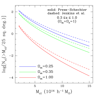
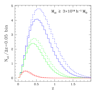
Figure 1: The expected number of clusters per square degree of sky, with redshifts $z\leq 1,$ and mass $\geq M,$ for two representative low-density, flat cosmologies. The calculations are made using the Press-Schechter formalism. The rms mass fluctuations are normalized to the present-day cluster abundance.

The right panel of Figure 1 shows a dramatic decrease in the sky density of clusters with mass $M_{\rm lim}$ $\geq 3\times 10^{14}M_{\odot}$ as $\Omega_{\rm m}$ increases. Integrating the histograms out to $z=1$, we find a total cluster count of 2.15 per square degree for the $\Omega_{\rm m}=0.25$ cosmology and 1.14 per square degree for the $\Omega_{\rm m}=0.35$ cosmology. We can therefore calculate that $d\ln[N(\geq M_{\rm lim},z\leq 1)]/d\ln\Omega_{\rm m}=-1.88$ for our particular choice of cosmological parameters in the Press-Schechter formalism. It follows that $|\delta\Omega_{\rm m}/\Omega_{\rm m}|=0.53\delta N/N.$ Assuming Poisson statistics, a sky density appropriate for $\Omega_{\rm m}=0.3$, and 25 square degrees in the Supernova Cosmology Project (SCP) data base, we would expect to obtain about 41 clusters above our threshold mass for $\delta N/N=0.16$ and $\delta\Omega_{\rm m}/\Omega_{\rm m}=0.08$. It is therefore reasonable to expect $\sim 10\%$ precision in $\Omega_{\rm m}$ from a complete survey of just the SCP imaging database. This perhaps surprising figure arises from the number of clusters detectable by optical surveys, which is much greater than that obtainable through X–rays at high redshifts.

As discussed in §3, by increasing our sky coverage with other imaging databases, we can further improve these constraints. The limiting factors on our uncertainty in $\Omega_{\rm m}$ are the number of clusters found, our ability to evaluate the survey completeness function, the accuracy of our mass function model, and our ability to set a limiting mass threshold. The problem of measuring cluster masses accurately is common to all cluster surveys, and requires extensive follow-up observations. Redshifts obtained through the Hobby-Eberly telescope will help a great deal in this regard, but much more accurate masses can be obtained through weak lensing, X–ray spectroscopy, or combined analysis of X–ray and Sunyaev-Zel’dovich surface brightness maps. StaCSis currently pursuing all three options for follow-up of confirmed clusters.

2.2 The Importance of the Low-Redshift Constraint

An important aspect of the calculation depicted in Figure 1, alluded to but not fully explained above, warrants further comment. When the PS formalism is applied to the present-day density of rich clusters, which is thought to be well known, a degenerate constraint on $\sigma_{8}$ and $\Omega_{\rm m}$ is obtained. The constraint used in the calculation above, obtained by Borgani et al. (1999) for a flat universe, is

$$\sigma_{8}=(0.58\pm 0.06)\times\Omega_{\rm m}^{-0.47+0.16\Omega_{\rm m}}\,.$$ (5)

Equation 5 allows the amplitude of the fluctuation spectrum $P(k)$ to be determined for any chosen $\Omega_{\rm m},$ and thus allows $\sigma_{M}$ to be calculated for any cluster mass $M.$ By implication, our prediction of the number of intermediate redshift clusters is only as good as the low-$z$ normalization. There is now some reason to doubt it, though, as recent work (Postman et al., 1996; Holden, et al., 1999, 2000) has found tentative evidence that the low-redshift cluster abundance is considerably higher than indicated by the Abell Cluster Catalog (Abell, Corwin, & Olowin, 1989), long thought to be nearly complete to $z=0.2.$ It is not yet clear what these results may imply for the accepted normalizations such as Equation 5. They do, however, suggest that StaCS and other cluster search programs cannot necessarily assume a known low-$z$ normalization of $\sigma_{8},$ but rather must determine it self-consistently along with $\Omega_{\rm m}$ from the higher redshift cluster abundance data.

2.3 Determination of Virial Masses

An oft-neglected subtlety in applying the PS formalism is the precise definition of virial mass, the mass that properly is to be used in Eq. (2). Gravitationally bound objects are not, in general, truncated abruptly at a particular radius; instead, their density profiles $\rho(r)$ smoothly approach the background mean density $\overline{\rho(z)}.$ Hence, one cannot specify their mass without reference to a particular radius or overdensity. Eq. (2) applies specifically to the mass $M_{V}$ within a radius, $r_{V},$ with the property $3M_{V}/4\pi r_{V}^{3}=\Delta_{V}(z,\Omega_{\rm m},\Omega_{\Lambda})\overline{\rho(z)}.$ In an $\Omega_{\rm m}=1$ universe, $\Delta_{V}\simeq 178$ at all redshifts; for $\Omega_{\rm m}<1,$ $\Delta_{V}$ is larger than this value, and increases with decreasing redshift. Kitayama & Suto (1996) give analytic approximations to $\Delta_{V}(z)$ as a function of $\Omega_{\rm m}$ for flat and open cosmologies.

This definition of virial mass means that one cannot compute $M_{V}$ from observational data, such as galaxy velocity dispersion or X-ray temperature, without specifying both a cosmology ($\Omega_{\rm m}$ and $\Omega_{\Lambda}$) and a model for the radial mass distribution of the cluster. Willick (2000; hereafter W00) studied this issue for MS1054-03, a massive cluster at $z=0.83.$ He showed that one could convert velocity dispersion, X-ray temperature, and weak lensing data for this cluster to an accurate virial mass if (1) a mass profile of, e.g., the type advocated by Navarro, Frenk, & White (1997) (NFW) was adopted (though any other simple analytical model would have worked just as well), and (2) the characteristic radius $r_{s}$ for this profile was taken as known. If no density profile was assumed a priori, the virial mass was determined only to within about 50%; even given the choice of the NFW profile the uncertainty was at least 20% (not counting observational uncertainties) without adopting a particular value for $r_{s}.$ The latter uncertainty is illustrated in Figure 4 of W00. W00 argued that preferred values of $r_{s},$ and thus of $M_{V},$ could be chosen by requiring that the cluster concentration index (essentially the ratio of $r_{V}$ to $r_{s}$) be in the relatively narrow range predicted from the N-body experiments of NFW. However, this constraint is, in truth, based on theoretical analyses not yet confirmed by detailed observational study.

W00’s analysis reinforced an issue that should be taken very seriously in future cluster analyses: The density profiles of clusters are crucial to determining the virial masses which enter into the PS formalism. And yet, we still are not certain whether the NFW profile, or any other analytic form, for that matter, are valid for a majority of rich clusters. This question relates to the broader and deeper issue of, What is the distribution of dark matter in gravitationally bound structures? Any analysis of clusters should pay as much attention to this question as to that of the evolution of the their abundance over cosmic times.

This is, then, a secondary goal of StaCS. The clusters we identify will be followed up by observations that aim to constrain cluster density profiles as well as measure mass. The most useful data for this purpose will be weak gravitational lensing data, which enable one to compute the run of cluster mass with radius out to the virial radius ($r_{V}\approx 1.5h^{-1}\,{\rm Mpc}$) and beyond. (By contrast, strong gravitational lensing, such as giant arcs, typically constrain the mass only within a few hundred kiloparsecs of the cluster center.) Such data are best obtained from space telescopes such as HST and, eventually, NGST, although the new generation of ground-based telescopes such as VLT and Gemini, with their much larger fields of view and promise of image quality approaching that of the HST, may end up being as well or better suited to this purpose. Galaxy velocity data and X-ray data obtained using Chandra can also shed light on this problem, and we will pursue these avenues as well. By publishing our StaCS clusters following spectroscopic confirmation, we hope that community follow-up will lead to the acquisition of such data. The long-term goal of accurately measuring the mass distribution in rich clusters is of necessity the task of many scientists pooling observational resources.

2.4 A Breakdown of Press-Schechter?

In important issue for StaCS, and indeed for any program that uses clusters as cosmological probes, is the possible breakdown of the PS approach at masses and epochs such that $\nu_{M}=\delta_{c}(z)/\sigma_{M}\gg 1.$ The PS formalism suggests that such objects are exponentially rare, with abundance $\sim\nu_{M}e^{-\nu_{M}^{2}/2}.$ As a result, the existence of very massive ($M\gtrsim 10^{15}\,M_{\odot}$) clusters at redshifts approaching unity, such as the X-ray clusters MS1054–03, has been taken as prima facie evidence for low $\Omega_{\rm m}$ (Bahcall & Fan, 1998; Donahue et al., 1998) or as possible evidence for non-Gaussian initial conditions (W00).

Only recently have there been cosmological N-body simulations of large enough volumes to test PS in this regime. While these quite recent results should be considered preliminary, it now appears that the PS formula, Eq. (2), does indeed break down in the sense that it underpredicts the abundance of the most massive clusters, especially at moderately high ($z\sim 1$) redshift (Gross et al., 1998; Governato et al., 1999; Jenkins et al., 2000). This departure from the PS predictions means that quantitative conclusions drawn from a small number of massive, high-redshift clusters, such as those discussed in the previous paragraph, cannot be correct in detail.

The failure of Press-Schechter for the rarest objects does not mean that clusters cannot be used as cosmological probes. For one thing, recent analytic work to improve upon PS has led to alternative formulae that more accurately predict the cluster abundance at the high-mass end (Sheth, Mo, & Tormen, 1999; Sheth & Tormen, 1999). It these formulae are confirmed, one can derive cosmological constraints from cluster abundance data using the new formulae rather than the PS expression. For another, it still appears that the PS formalism performs well in the intermediate cluster mass regime ($M\approx 3$–$5\times 10^{14}\,M_{\odot}$), where the majority of intermediate redshift clusters are found in any case.

Thus, the cosmological tests we propose to do with StaCS, and that are planned with other cluster surveys, remain viable. However, we and other workers must take great care, in the analysis phase, to account for departures from the familiar Press-Schechter formalism that now, apparently, occur at the high-mass end. New theoretical developments in this subject are certain to emerge in the coming years, and we will follow them closely.

3 Image Analysis and Cluster Identification

We begin with existing archival imaging databases that cover a significant area ($\lower 2.15277pt\hbox{$\buildrel>\over{\sim}\,$}10\,\Box^{\circ}$) of the sky, and are complete to a limiting magnitude of $m_{R}\simeq 23.5.$ The most important imaging database we use is that obtained by the Supernova Cosmology Project (SCP; Perlmutter et al., 1999). The SCP images were obtained as part of a search for distant supernovae, but are suited to identifying intermediate redshift clusters as well. The SCP imaging database currently covers approximately 25 square degrees of sky (see below). We are also working, in collaboration with M. Postman, with images from the DEEPRANGE survey (Postman et al., 1998), which covers 16 square degrees of sky, and with images from the ESO Imaging Survey (Nonino, et al., 1999 ), which covers 24 square degrees of sky. This total database of over 60 square degrees to $m_{R,lim}\lower 2.15277pt\hbox{$\buildrel>\over{\sim}\,$}23.5$ will enable us to detect many ($\sim 50$–100) rich clusters, with nearly 100% detection effeciency, in the redshift range $z\simeq 0.3$–$1.0$.

3.1 Data Reduction Procedures

In this section we describe the steps required to go from raw CCD images, acquired from the archival imaging databases described in §3, to catalog of cluster candidates with estimated masses and redshifts. We use a variety of publically available and commercial data-processing software in this process, including IRAF, STSDAS, FOCAS (Jarvis & Tyson, 1981), SEXTRACTOR, and IDL, plus locally written software.

3.1.1 Galaxy catalog generation from deep images

The images we obtain from the SCP or EIS archives are already flatfielded and sky-subtracted. Thus, the first stage in the image reduction is stacking and coadding several frames to reach the required limiting magnitude $m_{R}\sim 23.5$ required for completeness to $z\simeq 1.$ Typically 4 or more frames with small dithers are coadded. Registration and coadding are accomplished using the IRAF package IMMATCHX. We have found that the distortions in a typical prime focus image are large enough that generating mosaics is impractical, so we have used coadded frames from sets of images shifted no more than a few tens of arcseconds. Given the nature of the SCP data base, the images were taken over more than one observing run, separated in time by a month or more.

Following the generation of coadded frames, we run a sequence of FOCAS tasks that identify and categorize objects. FOCAS produces a list of galaxies and stars, with positions in CCD coordinates and preliminary magnitudes. We then employ locally written software to carry out astrometry and accurate photometry. We use the USNO-A2.0 astrometric catalog which 30–150 unsaturated objects per frame to tie each coadded CCD frame to an J2000 astrometric system. Typical rms positional errors are $0\farcs 5.$ Our photometry package improves upon FOCAS in several ways:

1. We have forced the FOCAS routines to adopt the initial sky subtraction carried out by the SCP for object identification and moment calculations. For our own photometry routine, we fit a planar sky to the frame, since the initial SCP sky subtraction was globally accurate only to $\sim 0.2\sigma_{sky}$. The planar fit removes small, large-scale gradients in the residual sky. We also compute a local sky for each object in the catalog, using it in favor of the global fitted sky unless there are too few pixels or the local sky shows too much variance.

2. All stars on the frame are masked prior to galaxy photometry, and any portion of a galaxy light profile in a masked region is properly compensated for with a symmetrically located pixel in the galaxy profile.

3. We carry out photometry within a series of elliptical apertures, stopping when the surface brightness along an elliptical contour drops below the sky error. The aperture photometry is then extrapolated to a total magnitude using the method of moments described by Willick (1999).

4. A useful step, we have found, is to flag and correct certain objects that have been erroneously classified as galaxies by FOCAS. We plot total magnitude versus effective surface brightness for all objects on a frame. Stars fall on a locus defined by a tight $m$–SB relation of slope unity, and at $R\lesssim 20.5$ fall on a well-defined locus with a higher surface brightness than galaxies. We reject those stars from the galaxy catalog produced by FOCAS. Close binary stars and bright stars near (but below) the saturation limit both can be eliminated from the galaxy lists in this manner. For $R>20.5$, the star and galaxy distributions are merged, but the galaxies outnumber stars by a large factor and we have kept the FOCAS star/galaxy classifications (cf. Kawasaki et al., 1998).

5. Saturated stars, bright stars off the edge of the frame, and the increased noise near the edge due to dithering cause both spurious and unidentified objects. We catalog these regions by creating (by hand) a set of exclusion boxes for each frame, including an indication of how close to the edge reliable galaxy identifications are found. While our algorithm for chosing these exclusion regions is somewhat qualitative, we have found the procedure promotes consistency and eliminates some spurious features in the galaxy luminosity functions and the cluster likelihood maps (${\cal L}_{\rm fine}$  defined in §3.2.).

Our final galaxy catalog for a given frame thus consists of CCD $(x,y)$ coordinates; RA and DEC accurate to $0\farcs 5$ for brighter galaxies, $m_{R}\lower 2.15277pt\hbox{$\buildrel<\over{\sim}\,$}21,$ and to $\sim 1\farcs 0$ for fainter objects; total magnitude and its estimated error; and several auxilliary pieces of information: effective surface brightness and radius, position angle, and ellipticity. These auxiliary data are not used in the cluster finding procedure (see below) but may be of interest at a later time.

For both the SCP and EIS databases, we generally reduce multiple ($\sim 5$–$20$), slightly overlapping frames, which we then combine into a single catalog covering from $0.2$–1 square degree. When combining we attempt to ensure that a given galaxy appears only once in the final catalog. This is important, as multiple appearances of single galaxies in the overlap regions can produce a spurious clustering signal. The positional and photometric parameters of the final catalog objects are obtained by averaging the corresponding parameters of the galaxies that appear in more than one input catalog. Objects found on different input frames with coordinates that differ by $\leq 2\farcs 0$ are judged to be the same galaxy and are combined. This nearly always yields the desired elimination of duplicates, though on occasion we find faint, low-surface brightness objects near the frame edges that appear twice in the final catalog. However, the numbers involved are small and the task of automatically identifying these cases difficult so we have not attempted a more sophisticated algorithm.

During the combination of multiple frames’ galaxy catalogs we also remove objects within each frame’s exclusion boxes. A set of exclusion boxes for the final catalog consists of the logical union of box area associated with each individual frame followed by the combination between frames with a logical intersection.

3.2 Application of the Matched Filter Algorithm

We search the galaxy catalogs for candidate clusters using a matched filter algorithm (MFA). Our implementation of the MFA, clusterfind, closely follows the methods of Kepner et al. (1999), except where specifically noted below. Readers are referred to Postman et al. (1996), Kawasaki et al. (1998), Kepner et al. (1999), and Kepner & Kim (2000) for more extensive discussions of the MFA, but for the sake of completeness we present an outline of the approach below.

3.2.1 Models of the Field and Cluster Galaxy Distributions

The MFA approach begins with a model for the number of galaxies at angular distance $\theta$ to within $d\theta$ of a cluster center, and having flux $l$ to within $dl:$

$$n(\theta,l;z)\,2\pi\,\theta\,d\theta dl=\left[n_{f}(l)+{\cal R}n_{c}(\theta,l;z)\right]\,2\pi\,\theta\,d\theta\,dl\,.$$ (6)

Here, $n_{f}(l)$ is the background or “field” galaxy contribution, which is assumed to be spatially uniform (but see below), and ${\cal R}n_{c}(\theta,l;z)$ is the cluster contribution. The factor ${\cal R}$ represents the overall “richness” of the cluster, to be defined more precisely below.

Aside from the richness factor, all clusters at a given $z$ are assumed to be identical. That is, $n_{c}(\theta,l;z)$ is a universal function, which we take to be a truncated Plummer law in space multiplied by a Schechter (1976) luminosity function. Following Kepner et al. (1999) we require that $n_{c}$ be normalized in the sense that

$$2\pi\int\theta d\theta\int dl\,n_{c}(\theta,l;z)L(l,z)=L^{*}\,,$$ (7)

where $L^{*}$ is the characteristic luminosity in the Schechter function. With this definition, it follows that the richness ${\cal R}$ is the cluster luminosity in units of $L^{*}.$ Imposing this normalization we find that $n_{c}$ is given by

$$n_{c}(\theta,l;z)=\frac{\left[\left(1+\frac{\theta^{2}}{\theta_{c}^{2}}\right)^{-1}-\left(1+y^{2}\right)^{-1}\right]\left(\frac{l}{l^{*}}\right)^{-\alpha}e^{-l/l^{*}}}{\pi\theta_{c}^{2}l^{*}\left[\ln(1+y^{2})-\frac{y}{1+y^{2}}\right]\Gamma(2-\alpha)}\,,$$ (8)

where:

• $\alpha$ is the faint end slope of the Schechter luminosity function;

• $y\equiv r_{max}/r_{c},$ where $r_{c}$ is the cluster core radius and $r_{max}$ is the truncation radius;

• $\theta_{c}=r_{c}/d_{A}(z),$ where $d_{A}(z)$ is angular diameter distance;

• $l^{*}=L^{*}/4\pi d_{L}^{2},$ where $d_{L}$ is luminosity distance (in practice, $l^{*}$ is further corrected for K-correction and Galactic extinction as discussed below);

• and $\Gamma(x)=\int_{0}^{\infty}t^{x-1}e^{-t}dt$ is the usual Gamma-function.

We discuss specfic choices of $\alpha,$ $L^{*},$ $r_{c},$ $r_{max},$ $d_{A},$ and $d_{L}$ in the next section.

For the field galaxy distribution we adopt a power-law model,

$$n_{f}(l)=l_{f}^{-1}\left(\frac{l}{l_{f}}\right)^{-\beta}\frac{N_{f}}{\theta_{f}^{2}}\,.$$ (9)

For a Euclidean universe one expects $\beta=2.5;$ in practice we find $\beta\approx 2.0$ in the magnitude range of interest. The quantities $l_{f},$ $N_{f},$ and $\theta_{f}$ are not independent, and in practice, we fix $\theta_{f}=1\farcm 0$ and $l_{f}$ to correspond to $m_{R}=20.$ Then, only $\beta$ and $N_{f}$ remain to be determined, which we do on a catalog-by-catalog basis, as we explain further in §5.

3.2.2 Likelihood Maximization

Detecting clusters with the MFA entails maximizing the likelihood, given the above models for the cluster and field galaxy distributions, that a cluster lies at a given sky position and redshift. This likelihood is calculated on a grid of trial positions, $(\alpha_{i},\delta_{j},z_{k}),$ where $\alpha$ and $\delta$ are RA and DEC in decimal units and $z$ is redshift. The spatial grid $(i,j)$ runs over the portion of sky covered by the galaxy catalog with some desired resolution, and the redshift grid $k$ over the range of redshifts at which one expects to find clusters. We let $z_{k}=0.2,0.3,...,1.0,$ which provides sufficient redshift discrimination. At redshifts greater than 1, $l^{*}$ falls below our detection threshold and the completeness of the matched filter algorithm falls off rapidly. At redshifts less than 0.2, the survey volume is small and no new detections are expected.

Kepner et al. (1999) and Kepner & Kim (2000) show that one can detect clusters by maximizing either “coarse” or “fine” likelihoods. The former are less accurate, but are less computation-intensive to calculate. Kepner et al. (1999) suggest that the coarse likelihood be used for a first pass through the data set, and the fine likelihood used to refine the calculation for candidate clusters detected in the first pass. However, our catalogs are considerably smaller than those anticipated by Kepner et al. (1999), and thus we use only the fine likelihood. clusterfind then requires about 4 hours of CPU time per square degree of catalog searched on a Sparc Ultra 5 with a 270 MHz processor, a modest computational cost.

The fine likelihood ${\cal L}_{\rm fine}$ is the log of the Poisson probability that galaxies are found at their observed locations given the presence of a cluster of richness ${\cal R}$ at position $(\alpha,\delta,z)$ (cf. Kepner et al. (1999) who define ${\cal L}_{\rm fine}$ as the Poisson probability and work with log(${\cal L}_{\rm fine}$)). It is given by

$$\mbox{${\cal L}_{\rm fine}$}=\left[\sum_{i=1}^{N}\ln\left[n_{f}(l_{i})+{\cal R}n_{c}(\theta_{i},l_{i};\alpha,\delta,z)\right]\right]-N_{e}\,,$$ (10)

(Kepner et al., 1999), where the sum runs over all galaxies in the catalog, and $N_{e}$ is the total expected number of galaxies in the data set,

$$N_{e}=2\pi\!\int\theta\,d\theta\int_{l_{min}}^{\infty}(n_{f}+\mbox{${\cal R}$}n_{c})\,dl$$ (11)

where $l_{min}$ is the flux limit of the catalog. If, following Kepner et al. (1999), we now define

$$\delta_{i}=\frac{n_{c}(\theta_{i},l_{i})}{n_{f}(l_{i})}\,,$$ (12)

we find after some algebra a simpler expression for the fine likelihood:

$$\mbox{${\cal L}_{\rm fine}$}=\left[\sum_{\theta_{i}\leq\theta_{max}}\ln(1+{\cal R}\delta_{i})\right]-{\cal R}\eta\,,$$ (13)

where

$$\eta\equiv\frac{\gamma(1-\alpha,l_{min}/l_{*})}{\Gamma(2-\alpha)}$$ (14)

where $\gamma$ and $\Gamma$ are the usual incomplete and complete Gamma-functions. (The specific form of the quantity $\eta$ results from integrating the Schechter function from $l_{min}$ to infinity, giving the relative number of expected galaxies in the sample. There is nothing fundamental about Eq. (14) to the MFA algorithm.)

We have modified Eq. 13 to accomodate the exclusion boxes associated with our real galaxy catalogs. For each point in RA,DEC,$z$ space, the second term on the right-hand side (${\cal R}\eta$) is multiplied by an additional factor $\epsilon^{-1}$ such that $\epsilon$ is the spatial integral over the assumed normalized spatial distribution (truncated Plummer law) within $\theta_{max}$ that is external to the exclusion boxes. This extra factor therefore corrects for areas in which galaxies could not be detected even if they were present. This exclusion box correction eliminated a great deal of spurious signal in the ${\cal L}_{\rm fine}$ map near frame edges and saturated stars, increasing the effective area of the survey by about 10% and allowing for a more accurate determination of candidate parameters near the affected areas.

At a given grid position $(\alpha,\delta,z),$ we maximize likelihood by setting $\partial\mbox{${\cal L}_{\rm fine}$}/\partial{\cal R}=0.$ This leads to the equation

$$\sum_{\theta_{i}\leq\theta_{max}}\frac{\delta_{i}}{1+{\cal R}\delta_{i}}-\eta=0\,.$$ (15)

The value of ${\cal R}$ which solves this equation is then substituted back into Eq. (13) to obtain the final value of ${\cal L}_{\rm fine}$ at that position. As noted by Kepner & Kim (2000), Eq. (15) requires a numerical solution, which can be fairly time consuming, especially as it must be done at each grid point. Indeed, this is one reason that Kepner et al. (1999) advocate that the coarse likelihood be used first. We have written code to solve Eq. (15) that uses the Numerical Recipes (Press et al., 1986) algorithm ZBRENT, and is sufficiently rapid so as not to be a major bottleneck in clusterfind.

3.2.3 Using ${\cal L}_{\rm fine}$ to identify clusters

The procedure above produces three three-dimensional maps, $\mbox{${\cal L}_{\rm fine}$}(\alpha_{i},\delta_{j},z_{k})$, ${\cal R}(\alpha_{i},\delta_{j},z_{k})$, and $\epsilon(\alpha_{i},\delta_{j},z_{k})$. Cluster candidates are found by searching the ${\cal L}_{\rm fine}$ map for local maxima that satisfy the following conditions. First, we consider only ${\cal L}_{\rm fine}$ values where the corresponding richness value is positive and where the exclusion boxes correction factor $\epsilon>0.5$. A deficit of galaxies in a region of the catalog will generate a high value of ${\cal L}_{\rm fine}$ with a negative richness; adoption of $\epsilon^{-1}$ into Eq.(13) largely corrects this effect for deficits caused by data artifacts (and indicates where missing data is excessive), but there are nevertheless true underdense regions caused by large scale structure. Second, the 95th percentile ${\cal L}_{\rm fine}$ value is found for each $z$ plane of the ${\cal L}_{\rm fine}$ map (the ${\cal L}_{\rm fine}$ value in grid points with ${\cal R}<0$ is set to zero beforehand) and used as a threshold. We consider only local maxima at or above this significance level. Finally, we require that a local maximum be found, at or above the 95% significance level, at the same RA and DEC for three successive trial redshifts, e.g., at $z=0.3,0.4,0.5$. This last condition is imposed to remove extremely marginal peaks from consideration. When a candidate meeting the above criteria is found, we determine its estimated redshift by finding the maximum in the ${\cal L}_{\rm fine}$ versus $z$ curve at the maximum likelihood sky position.

Once candidates meeting the above criteria are found, we subject them to two further tests. First, the image(s) are inspected at the position of the cluster candidate. An overdensity on a spatial scale appropriate to the estimated redshift must be visually apparent. Second, we produce a background-subtracted luminosity histogram for the putative cluster within $r_{core}$, $2r_{core}$, and $4r_{core}$. A reasonable excess approximating a Schecter function must be apparent to the eye and in the local luminosity function if the redshift and richness estimates are to be believed. Although such visual tests subjective, they are still necessary if artifacts are to be avoided. As will be demonstrated in §4, most candidates identified with the automatic criteria pass the subjective visual tests.

4 A Worked Example: First StaCS candidates and confirmed clusters

Our first step, as noted in § 3, is to search the SCP data base for sets of images that coninuously cover a reasonably large patch of sky—a few tenths of a square degree or more. An example of such a set of images is shown in Figure 2, which shows all SCP frames covering a patch of sky centered on ${\rm RA\/}\approx 1\fh 0,$ ${\rm DEC\/}\approx 4\fdg 4$ (hereafter called the 01+04 field). The large blue boxes represent CTIO prime focus frames, which are the ones used in our analysis. The smaller boxes represent follow-up images, acquired at other telescopes, with smaller fields of view, that we do not use; the small gain in image depth achieved does not warrant the significant additional effort required to co-add images from different telescopes.

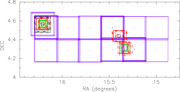
Figure 2: Positions of the CCD images obtained by the SCP in the 01+04 field (see text). The regular array of blue squares (CTIO prime focus frames taken in October and November 1995) have been processed with the full StaCS analysis procedure; the others were supernova follow-up frames and are not useful for StaCS.

4.1 Production of the Galaxy Catalog

At each of the 12 frame positions shown in Figure 2, we combine the individual CCD images to produce a single deep frame with a typical effective exposure time of $720\,s.$ For each of the 12 deep frames thus generated, we determine the best sky value, run FOCAS (tasks setcat, detect, sky, skycorrect, evaluate, and splits) with the sky and sky noise fixed, using a detection threshold of $2\times\sigma_{sky}$ and a minimum detection area of 4 pixels, use IRAF tools to identify 10-20 stars to set the FOCAS catalog point spread function with setpsf, and finally run the FOCAS task resolve. This results in a catalog of galaxy and star positions and magnitudes for each frame.

The photometric zero point for the magnitudes is obtained from the SCP data base and is accurate to $\sim 0.1$ mag or better. With the established FOCAS identifications we repeat the object photometry with a more sophisticated algorithm using local software. The individual catalogs are then mapped to celestial coordinates by matching objects within them to the USNO astrometric catalog (we do not discriminate between stars and galaxies for this procedure, as many USNO catalog soures are galaxies). The individual catalogs, now photometrically and astrometrically calibrated, are then combined to form a single catalog for the entire imaged region shown in Figure 2. Although there is significant spatial overlap among the deep frames, our combination algorithm ensures that very few duplicate objects remain in the final catalog and that the exclusion boxes are propagated to the final catalog correctly. One final step is to correct for galactic extinction using the Schlegel, Finkbeiner, & Davis (1998) dust emission maps and extinction calibration. Although most of the SCP fields were located in regions of low extinction, correcting for it changes the estimated $z$ and ${\cal R}$ values and in some cases noticeably corrects galaxy density variations caused by dust.

Figure 3 shows the positions of bright ($m_{R}\leq 20,$ approximately 1200 objects) and faint ($20.0\leq m_{R}\leq 23.0,$ approximately 22,000 objects) subsets of the galaxies in the final catalog. (For clarity, an additional $\sim 15,000$ galaxies with $m_{R}>23$ are not shown in the Figure.) The bright subset is shown by blue circles with size proportional to brightness; the brightest galaxies have $m_{R}\sim 17.$ The faint subset is shown as (red) dots of fixed size. The exclusion boxes are in black. The boxes in amongst the galaxies generally indicate the effects of saturated stars, while the boxes around the periphery identify for clusterfind the edges of the galaxy catalog.

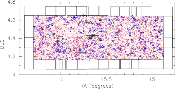
Figure 3: Positions of a subset of the galaxies detected in the CTIO prime CCD frames shown in Figure 2. Blue markers are sized according to the magnitudes of those galaxies with $m_{R}\leq 20$, and galaxies with $20<m_{R}<23$ are shown with red dots. Exclusion boxes are in black.

4.2 Determining the Background Galaxy Distribution

The next step is to determine the parameters of the power-law distribution of background galaxies, Eq. (9) above. Note first that if we adopt $\theta_{f}=1\farcm 0$ and take $l_{f}$ to be the flux corresponding to $m=20,$ Eq. (9) is equivalent to the statement that the total number of catalog galaxies brighter than apparent magnitude $m$ is

$$N(<m)=\frac{N_{f}\,\Omega_{{\rm eff}}}{\beta-1}\,10^{0.4[\beta-1](m-20)}\,,$$ (16)

where $\Omega_{{\rm eff}}$ is the effective solid angle of the catalog (i.e., the total area minus the combined areas of patches where bright stars precluded galaxy detection). Thus, the slope of the $\log N(<m)$ versus $m$ graph is $0.4(\beta-1),$ while the amplitude of the graph determines $N_{f}.$ In particular, for $\beta\approx 2$ (see below), $N_{f}$ is essentially the number of galaxies per square arcminute brighter than $m=20.$

In practice the power-law distribution of field galaxies is not realized over the entire range of apparent magnitudes. At the bright end, the number counts are biassed by small number statistics and the loss from the catalog of galaxies brighter than $m_{R}\sim 16$ due to detector saturation, and can either exceed or fall short of the power-law expectation. At the faint end, incompleteness sets in above $m_{R}\sim 23.$ To quantify this, we fit the power-law only over a range of magnitudes, $19\lower 2.15277pt\hbox{$\buildrel<\over{\sim}\,$}m_{R}\lower 2.15277pt\hbox{$\buildrel<\over{\sim}\,$}22.5,$ with the exact range chosen on a case-by-case basis. Brighter than this range, we do not fit the number counts. Fainter than the chosen range, we multiply the power law by an incompletness function, which we take to have a Fermi-Dirac form,

$$g(m;m_{c},\Delta m)=\left[1+e^{(m-m_{c})/\Delta m}\right]^{-1}\;,$$ (17)

where $m_{c}$ is a characteristic cut-off magnitude and $\Delta m$ represents the sharpness of the cut-off. Note that we use the exclusion boxes at this stage both to remove from consideration spurious objects and to measure properly the area of sky observed. Processing the catalog without the exclusion boxes gives inconsistent results, both with respect to the number density normalization and the shape of the distribution at the faint end.

Figure 4: Total number of catalog galaxies as a function of apparent magnitude, for the SCP fields shown in the previous figures. The solid line represents the measured counts, while the dashed line is the fitted power law (Eq. 16) multiplied at the faint end by the incompleteness function (Eq. 17).

Figure 4 shows the results of carrying out this procedure for the catalog derived from the frames shown in Figure 2. The fitted parameters for the power-law distribution, $N_{f}$ and $\beta,$ are indicated on the figure, as are those of the incompletness function. The indicated values of $N_{f}$ and $\beta$ are consistent with what we find in other SCP fields, though they vary from field to field, possibly due to errors in the photometric zeropoint or variations in seeing causing slight differences in the efficiency of star-galaxy identification. Note that the width of the incompleteness cutoff, $\Delta m\approx 0.25,$ is quite small. For this reason, when we apply clusterfind, we consider only galaxies with $m\leq m_{c},$ and assume that the formalism of a strict magnitude limit, implicit in Eqs. (10–15), is a good description of the data. This simplification means clusterfind loses some signal we could potentially gain by including galaxies just past the faint limit, and it also means the equation for the background galaxy distribution overestimates the catalog number density just short of the faint limit. An alternative would be to use all the galaxies, and to incorporate the incompleteness function, Eq. (17), into the MFA formalism. However, this would complicate the mathematical expressions involved as well as introduce a higher fraction of spurious objects, and we have judged it not to be worth the added complexity.

4.3 Identification of cluster candidates

The next step is to apply clusterfind to the galaxy catalog. This requires that we adopt values for the model parameters on which the algorithm of §3 depends; our choices are shown in Table 1. Only the field galaxy distribution parameters $\beta$ and $N_{f},$ and the magnitude limit $m_{lim},$ are newly determined for each catalog. The other parameters, in particular those describing the cluster properties, are hardwired to the values given in Table 1. The cluster galaxy luminosity function was estimated from data in Driver, Couch, & Phillipps (1998) based on our assumed cosmology. We execute the algorithm using observed quantities; the final result does not depend upon $h$ except through the explicit $M^{\ast}$, $r_{core}$, and $r_{max}$ dependencies listed in the table. We have adopted the $r_{max}$ used by Postman et al. (1996) and Kepner et al. (1999), but have used a larger $r_{core}$.

The K-correction is problematic for the SCP data, since the fields primarily consist of $R$-band images and we cannot estimate a spectral type except for low redshift galaxies in the sample. We therefore have applied a mean K-correction to all the galaxies equally based on an average of functions taken from Coleman, Wu, & Weedman (1980). While this will give increasing errors in galaxy magnitudes with redshift, we note that the detection of a cluster is based on the combination of the local apparent luminosity function excess and the angular scale size of the overdensity, but the latter is weakly dependent on $z$ at high redshifts (and moreover depends on both the specific cosmology and possible evolution in the scale size of clusters, both of which we have fixed). Therefore, a systematic error in the adopted K-correction will give systematic but small errors in predicted $z$. Because we do not intend to do science with the un-confirmed cluster catalog, the estimated $z$ values will be used only to prioritize the targets and to chose the best spectroscopic configuration (choice of grism, filter, etc.).

As noted in §3, the output of clusterfind consists of maps of the likelihood ${\cal L}_{\rm fine}$ and richness ${\cal R}$ on the plane of the sky ($\alpha,\delta$) and at each of 9 redshifts, $0.2,...,1.0.$ Figure 5 shows the ${\cal L}_{\rm fine}$ map for the region in question. The likelihood map is searched for peaks that lie above a 95% threshold (i.e., that have ${\cal L}_{\rm fine}$ in the top 5% of values at that redshift) at three consecutive redshift planes. In Figure 6 we plot, for six such peaks derived from the 01+04 field, ${\cal L}_{\rm fine}$ versus redshift. In Figure 7 we plot the local excess apparent luminosity function for the same peaks within concentric circles around the candidate position.

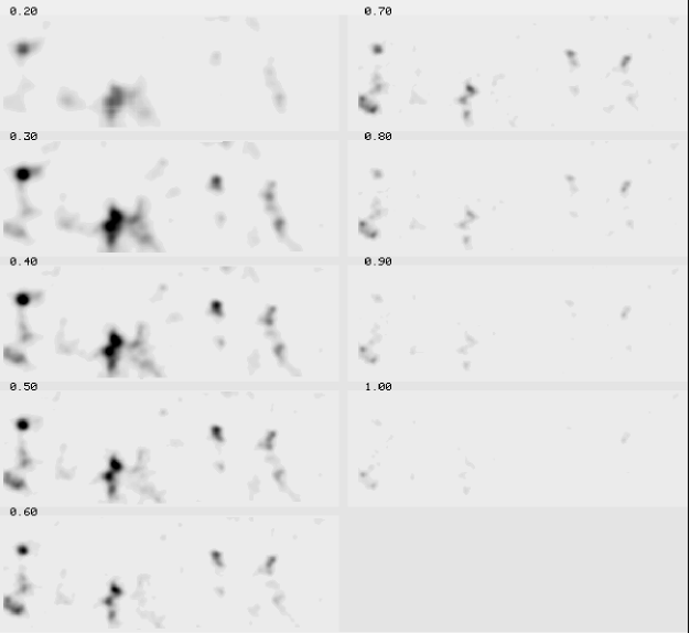
Figure 5: The 3-dimensional ${\cal L}_{\rm fine}$ map resulting from a run of clusterfind on the 01+04 field galaxy catalog. The redshift for each RA-DEC plane is shown in the upper left hand corners. Values of ${\cal L}_{\rm fine}$ are suppressed (set to -1 in the plot) where ${\cal R}<0$. The confirmed cluster J0104.8+0430 is represented by the strong, nearly circular peak in the upper left hand corner.

Figure 6: Likelihood ${\cal L}_{\rm fine}$ versus redshift for six candidate clusters obtained from the 01+04 field. The peak of each curve indicates the most probable redshift of the candidate cluster, and the richness at the peak its estimated richness. The dotted lines represent the 95${}^{\mbox{th}}$ percentile ${\cal L}_{\rm fine}$ value as a function of redshift, used as a threshold (see text).

Figure 7: Luminosity functions for the candidates indicated in Figure 6. The horizontal axes are $R$-magnitude and the vertical axes are the integrated excess number counts ($N(<m)-N_{background}(<m)$) within circles centered on the cluster candidate. The solid lines indicate the counts within $r_{core}$ of the center, dotted within $2r_{core}$, and dashed within $4r_{core}$. The background distribution is assumed to be the straight power law used in clusterfind, and exclusion boxes were ignored.

Table 2 shows the candidates from the 01+04 field that pass the tests noted.

4.4 Matched filter algorithm limitations and tests

Of 20 cluster candidates found with the MFA listed in Table 2, 11 appear to be associated with larger scale galaxy overdensities or substructure, largely confirmed by their apparent luminosity functions (see Figure 7). There are several reasons to be careful in the interpretation of MFA results without spectroscopic confirmation. First, the non-uniform background galaxy distribution effectively changes the threshold level (see Bramel, Nichol, & Pope, 1999), and since the ${\cal L}_{\rm fine}$ map is nonlinear, the rise of a local maximum above the surrounding ${\cal L}_{\rm fine}$ value is not necessarily indicative of what the cluster’s signal would be if seen against the mean background density. This may be somewhat ameliorated if we were to use a locally determined threshold when analyzing the ${\cal L}_{\rm fine}$ map, but nonlinearity in the ${\cal L}_{\rm fine}$ calculation would still give incorrect values for detected cluster candidates. Another approach is to use a local background galaxy distribution when calculating ${\cal L}_{\rm fine}$, but estimation of the background counts will be problematic, because of similarity in the scales of background density variations and cluster angular sizes.

A second problem with the MFA is that it assumes real clusters have a strongly peaked spatial distribution and there are no significant overdensities that are not clusters. Overdensities in the form of “sheets” and “strings” will also contribute to the ${\cal L}_{\rm fine}$ signal, and with projection effects we may identify candidates that are not massive bound structures. A third problem when searching for medium to poor clusters is that overlapping cluster candidates are common. The model for ${\cal L}_{\rm fine}$ is a single cluster on a uniform background, and the nonlinearity in the ${\cal L}_{\rm fine}$ value prevents effective deconvolution. This may, however, be a minor concern since cluster characteristics vary enough that such deconvolution could not be used even with a linear likelihood (such as ${\cal L}_{\rm coarse}$ from Kepner et al., 1999). In such cases a thorough spectroscopic redshift campaign is required; such ${\cal L}_{\rm fine}$ signals may indicate merging clusters or the projection of large scale structure elements.

We have taken the position that the MFA, particularly when used with single-band images, will not have sufficient information to identify true clusters with small and well-understood false positive rates and completeness properties. We therefore intend to use the MFA only to identify candidates, emphasize completeness over avoiding false positives, and confirm the clusters spectroscopically. It is further evident that we cannot reliably identify true clusters in some cases without thorough investigation of the velocity field to reject cases where projection of large scale structure, rather than gravitationally condensed clusters, provides the galaxy overdensity detected by ${\cal L}_{\rm fine}$. We also expect to find high redshift clusters projected behind low redshift clusters, and these may be unidentified without thorough analysis of the velocity field to faint limits. Merging clusters or collapsing proto-clusters may also show a large velocity dispersion, given a sparse sampling of galaxy redshifts, and give us an incomplete picture of the candidate. The use of deep images to find candidates is only the first step.

Since the matched filter algorithm implements a specific model for a cluster’s spatial galaxy distribution and luminosity function, it is reasonable to ask whether our detection efficiency is model-dependent. We have performed a preliminary analysis of this question by investigating the filter’s response to simulated clusters over a wide range of the parameters listed in Table 1. The ratio between a cluster’s peak ${\cal L}_{\rm fine}$ value and the 95th percentile ${\cal L}_{\rm fine}$ value (our detection threshold), appears robust under reasonable variations in the assumed background and member galaxy distributions. The real variations in cluster properties are therefore not likely to be an obstacle in assessing this survey’s completeness. Differences between the filter model and the properties of our simulated clusters do create systematic errors in the algorithm’s richness and redshift estimates, but these values are only used to prioritize our candidates for follow-up observations.

One fortuitous check on our algorithm is provided by MS 1054.4-0321 (Gioia et al., 1990; Stocke et al., 1991), re-discovered as STACS J1056.9-0337. At the time of those particular SCP observations (prior to March 1997), the choice of fields sometimes included known high redshift clusters to boost the probability of finding supernovae, so this re-detection cannot be included in a formal StaCS statistical sample. It can, however, be used to check our parameter estimation accuracy. Our algorithm found $z_{est}=0.7$, ${\cal R}=83.5$, and the peak ${\cal L}_{\rm fine}$ value was a factor of 16 above the (95th percentile) threshold. Tran et al. (1999) found $\langle z\rangle=0.833$, indicating our estimated redshift is more than one $z$-step low. Our $\cal R$ represents a direct fit to an observable, and therefore is a valid measure of the cluster, but the number quoted is based on $z_{est}=0.7$; going back to the $\cal R$ map and interpolating we find ${\cal R}(z=0.833)\sim 160$. Use of $\cal R$ is a good simple method of estimating the optical luminosity, since it subtracts the background galaxy distribution and it weights the galaxies in both radius and magnitude according to our Schechter function + Plummer law cluster model rather than having hard cutoffs in magntiude and radius. However, real clusters are not round (this one manifestly so), they may be projected against an over- or underdense region of background galaxies, and they may not have a Schechter luminosity function (e.g. may have a CD galaxy at the center which adds greatly to the luminosity but does not affect $\cal R$ proportionally), so a proper luminosity measurement must identify cluster members more accurately.

The underestimate of $z$ for high redshift clusters may be systematic in origin. This might come from a K-correction error (an overestimate of the effective value), an error in the assumed cosmology (this could account more than half a magnitude, cf. Figure 1 of Perlmutter et al. 1999, which can give errors of $\sim 0.1$ in redshift), or an evolving luminosity function. As the catalog of confirmed clusters grows we will be able to determine whether such errors are systematic or random.

As expected, MS1054.4-0321 is the richest cluster dectected out of $\sim 3\,\Box^{\circ}$ processed. The encouraging aspect is that much poorer clusters have significant ${\cal L}_{\rm fine}$ signal as well, even with our single filter images. We have tens of candidates with optical luminosities (as indicated by ${\cal R}$) within a factor of a few of MS1054.4-0321, and we can expect deep optical surveys such as StaCS to have a high degree of completeness at mid- to high richness.

4.5 Spectroscopic results

During the first season of science operations of the HET, we confirmed a cluster candidate in the 01+04 field with the Marcario Low Resolution Spectrograph (Hill et al., 1998) in longslit mode. The spectra were taken in October 1999 with 2 arcsecond slits (resolution $\sim 600$) at various position angles allowing several galaxies per exposure. Figure 8 shows the spectra, including 5 cluster members, 1 likely member, and 3 unassociated galaxies. The data were reduced with IRAF apextract tasks and the redshifts measured with the rvsao package using SAO galaxy spectrum templates, although we have found that the galaxy templates from Kinney et al. (1996) are better for higher redshift galaxies due to their broader wavelength coverage. The mean redshift $\langle z\rangle=0.400$ of the 6 likely members is close to the $z=0.4$ value predicted by clusterfind.

Figure 8: Spectra of galaxies in the field of STACS J0104.8+0430. The solid lines are the spectra, smoothed with a 5-pixel boxcar filter (approximately the size of the resolution element), and the dashed lines are the approximate pixel uncertainties. The verical axes are roughly calibrated F_λ. The H+K absorption features are just short of the $\lambda 5577$ sky emission line subtraction residuals in the cluster members.

The current list of confirmed clusters is in Table 3. We have adopted a liberal criterion for the confirmed candidate list, requiring only 3 redshifts within 2000 km s^-1. Columns 6 and 7 give the number of redshifts in that range and the total number of redshifts that we know in the field, respectively; these numbers are indicative of the strength of our spectroscopic confirmation. We recognize that some of these candidates may indeed be rich groups, projections of large scale structure, or mere coincidences; we may also find a foreground group’s redshift has been determined instead of a true background cluster. Our target confirmation level for HET spectroscopy is to obtain on the order of a dozen member redshifts for each candidate before adding it to the StaCScluster catalogue. Extensive spectroscopy is required to confirm a virialized, massive structure, especially for poor and high redshift clusters where the background contrast is low. Follow-up observations of the confirmed catalogue are essential for most of our science goals.

An online version of the StaCS confirmed cluster catalog can be found at http://redshift.stanford.edu and will be updated as we obtain further HET data. We will also make available upon request the positions, redshifts, and spectra of galaxies in these fields. Those who would like to study these clusters further should contact KLT. As indicated in the introduction, StaCS may turn out to be more limited in scope than our original plan, and we will therefore not guard our data closely. The candidate list and software will be made available to any group wishing to continue the search or make use of our catalogue, which contains a wide variety of interesting high-redshift cluster candidates.

5 Conclusions

The purpose of this paper has been to describe StaCS, a new research program aimed at identifying previously unknown intermediate and high redshift galaxy clusters from moderately deep, archival CCD images covering several tens of square degrees of sky. These images were originally obtained by the Supernova Cosmology Project (Perlmutter et al., 1999) for the purpose of finding high-redshift supernovae. Our short term goals are to identify new clusters with a wide variety of masses in these images by using a matched filter algorithm that provides reasonably accurate estimates of cluster richnesses and redshifts. We then follow up viable candiates with HET spectroscopy to measure redshifts and confirm that the objects are bona-fide clusters. Our long-term goal is to use the clusters as cosmological probes, and in particular to measure the cosmological density parameter $\Omega_{\rm m}$ and the amplitude of density fluctations to $\sim 10\%$ accuracy. This long-term goal cannot be carried out using the archival images and HET data alone, because it requires accurate estimates of the clusters’ virial mass, for reasons outlined in §2. Additional observations will thus be needed, including multiobject spectroscopy at the HET and other 8 m class telescopes. If possible, we will also pursue X-ray, weak lensing, and Sunyaev-Zel’dovich observations, either ourselves or through collaboration, to measure cluster mass profiles. These observations will require the efforts of many workers, and we thus plan to make our cluster candidates available on the Internet for follow-up by the scientific community.

In this final section, we further discuss some recent key issues that will affect StaCS and similar projects.

5.1 Press-Schechter and Beyond

As noted in §2.4, the familiar Press-Schechter formalism for predicting the cluster abundance $n(M,z)$ has now been shown clearly to fail at the low and high mass ends (Governato et al., 1999; Jenkins et al., 2000), and more accurate analytic expressions for $n(M,z)$ have been proposed and tested (Sheth & Tormen, 1999; Sheth, Mo, & Tormen, 1999). Fitting formulas to the mass functions found in large-scale simulations are also becoming available (Jenkins et al., 2000) as an alternative to traditional models. There has not yet been a detailed study of the effect of changes in the model cluster mass function on cosmological constraints. The most comprehensive assessments of the power of the cluster abundance tests done to date are probably those of Romer et al. (1999) and Haiman, Mohr, & Holder (2000), both of which assumed the validity of PS in arriving at their findings. Haiman, Mohr, & Holder (2000), in particular, argued that extremely accurate constraints ($\sim 1\%$) on $\Omega_{\rm m}$ could be obtained from a $400$ square degree X-ray survey of clusters, even when variations on the nature of the cosmological constant (“quintessence”) are allowed. This high accuracy stems, in part, from the assumption that the theoretical predictions hold well into high-mass, high-redshift ($z>1$) regimes where PS apparently breaks down. It is not yet know whether the improved analytic formulae of Sheth & Tormen (1999) and Sheth, Mo, & Tormen (1999) will fully withstand scrutiny, in this regime of rare objects, as new N-body results come in.

We suggested in §2 that such uncertainty can be at least partially alleviated by focussing our efforts on the mass and redshift ranges where both the PS and the newer predictions are accurate. This means directing the abundance test at objects for which $\delta_{c}(z)/\sigma_{M}$ is not very large—which in practice means moderate cluster masses ($M\lower 2.15277pt\hbox{$\buildrel<\over{\sim}\,$}5\times 10^{14}\,M_{\odot}$) and redshifts ($0.3\lower 2.15277pt\hbox{$\buildrel<\over{\sim}\,$}z\lower 2.15277pt\hbox{$\buildrel<\over{\sim}\,$}1.0$). Such objects are, in any case, far more common than the high-mass, high-redshift clusters which could prove definitive if the PS formulae were rigorously correct. They are also diffulcult to detect in quantity through any means but an optical survey. Still, it is critical for the success of the cluster abundance test of cosmology that a better theoretical understanding of the evolution of $n(M,z)$ be reached.

5.2 Ancillary Scientific Goals

While surveys such as StaCS are aimed mainly at constraining cosmological parameters, especially $\Omega_{\rm m},$ this is not and should not be their only objective. It may turn out that other approaches to cosmological parameter estimation may prove more fruitful, although cluster evolution still provides a valuable independent constraint. The recent release of CMB anisotropy power spectra by the Boomerang (Lange et al., 2000) and Maxima (Balbi et al., 2000) teams has demonstrated the potential of CMB observations to carry out precision cosmology, and the coming year will see an order of magnitude improvement in these results with the Microwave Anisotropy Prove (MAP) satellite. If indeed CMB experiments live up to their potential and convincingly measure the cosmological parameters, what new insights will cluster surveys provide?

With $\Omega_{\rm m}$ and $\sigma_{8}$ already determined, a measurement of $n(M,z)$ out to $z\approx 1$ will be crucial in testing our theories of structure formation. Will $n(M,z)$ turn out to match N-body simulations, which will now have no remaining cosmological degrees of freedom? If not, the cluster abundance may be telling us something about a breakdown of other key assumptions about structure formation, such as Gaussianity of the initial conditions (e.g. Willick, 2000) or the dominant role of gravity in large-scale structure formation.

In addition, rich clusters of galaxies are excellent “cosmic laboraties” in which to test ideas about dark matter. Their mass distributions can be studied using X-ray, Sunyaev-Zeldovich (SZ), weak lensing, and redshift observations, and may be compared with the expected forms of dark matter halos. The fact that the halos around small galaxies do not appear to match the expectations from CDM simulations has been cited as evidence for self-interacting dark matter (Spergel & Steinhardt, 2000) and for warm rather than cold dark matter (Hogan & Dalcanton, 2000). However, surprisingly little is known about the dark matter distribution in clusters, and if such ideas are to be tested, we will need to learn much more about cluster halos. Cluster surveys such as StaCS will identify many new objects to study, at a wide range of masses and redshifts, that will bear on this important problem.

Indeed, as discussed in §2.3, a better understanding of cluster mass profiles is critical not only as an ancillary goal of StaCS, but to its primary goal of comsological parameter estimation as well. Ultimately one must estimate the virial masses of clusters in order to use them as cosmological probes, because it is in terms of virial mass that N-body experiments and analytical formulae, Press-Schechter of other, ultimately make their predictions. Because virial masses represent the mass enclosed within a given overdensity, some knowledge of the density profile is needed in order to go from observational data to virial mass. It has often been assumed that a single temperature measurement from X-ray data enables a direct inference of virial mass using simple, redshift-dependent formulae. This may be true in the future, but much work remains to be understood about the origin and evolution of the intracluster medium before such a mass-temperature relation can be applied with confidence (Mathiesen & Evrard, 2001). Similarly, weak lensing and velocity measurements of a cluster require a mass model to be converted into virial mass (Willick, 2000). A central goal of cluster surveys should be follow-up observations, using a variety of techniques, to constrain mass profiles and thereby obtain unbiased virial mass estimates. This has not been done in cluster surveys to date, and this may be one of the reasons for the discrepant cosmological conclusions drawn by the authors cited in §1 above.

We gratefully acknowledge the assistance of many: at LBL R. Quimby, G. Aldering, numerous others; at Stanford S. Church, R. Romani, V. Petrosian for useful discussions, students D. Sowards-Emmerd, D. Grin, F. Tam, E. Young, Y. Dale who contributed to software and/or data processing; at Univ. Sternwarte Göttingen: F. Hessman; at NOAO F. Valdez, M. Fitzpatrick; at McDonald Observatory special thanks to resident astronomers Grant. Hill, M. Shetrone.

The LRS is named for Mike Marcario of High Lonesome Optics who fabricated several optics for the instrument but died before its completion.

Table 1: Clusterfind Parameters.

Parameter	Value or range	Description
$\beta$	$\sim 2.0$	bckgd. dist. power law index
$N_{f}$	$\sim 0.6$	bckgd. density (arcmin-2) at $m_{R}=20$
$m_{lim}$	$\sim 23.2$–$23.6$	limiting magnitude ($\Leftrightarrow l_{min}$)
$M^{\ast}$	$-21.55+5\log{h}$	Schechter fcn. $L^{\ast}$ absolute R magnitude
$\alpha$	1.125	faint end slope of Schechter fcn.
$r_{core}$	0.25$h^{-1}$ Mpc	core radius of cluster
$r_{max}$	1.00$h^{-1}$ Mpc	truncation radius of cluster
$(\Omega_{\rm m},\Omega_{\Lambda})$	$(0.3,0.7)$	cosmological parameters (for calculating $d_{A},$ $d_{L}$)
gridspace	0.3 arcmin	spacing of grid points
E/S0:Sab:Sbc:Scd	4:3:2:1	ratio of galaxy type contribution to K-correction

Table 2: Cluster candidate list for the 01+04 field.

Name	Coordinates, J2000		Estimated parameters		Notes:
	RA (deg.)	Dec	$z$	${\cal R}$
STACS J0059.6+0437	14.9078	4.6250	0.9	29.9	1
STACS J0100.0+0433	15.0182	4.5600	0.8	20.2
STACS J0100.3+0417	15.0836	4.2900	0.3	14.2	2,3
STACS J0100.4+0427	15.1136	4.4600	0.6	37.7
STACS J0100.5+0424	15.1287	4.4100	0.4	18.9
STACS J0101.4+0428	15.3593	4.4800	0.4	28.6
STACS J0102.6+0413	15.6702	4.2250	0.3	13.2	2
STACS J0102.7+0421	15.6953	4.3600	0.4	13.1	2
STACS J0102.8+0414	15.7053	4.2450	0.3	12.1	2,4
STACS J0102.8+0415	15.7204	4.2550	0.3	11.4	5
STACS J0102.8+0418	15.7204	4.3050	0.3	15.9	2
STACS J0103.2+0419	15.8006	4.3300	0.4	37.5
STACS J0103.2+0414	15.8156	4.2350	0.3	24.4	2,6
STACS J0103.3+0416	15.8257	4.2800	0.4	35.7	2
STACS J0104.1+0430	16.0464	4.5100	0.8	10.6
STACS J0104.2+0416	16.0513	4.2750	0.8	35.0	6
STACS J0104.7+0420	16.1968	4.3400	0.5	25.2	2
STACS J0104.8+0422	16.2018	4.3800	0.5	20.5	2
STACS J0104.8+0430	16.2019	4.5000	0.4	38.0	7
STACS J0104.9+0414	16.2268	4.2400	0.6	50.6	2
STACS J0105.0+0415	16.2669	4.2600	0.6	42.3	2,5
STACS J0105.0+0417	16.2719	4.2850	0.7	66.9	2

Table 3: Confirmed cluster catalog

Name	Coordinates, J2000		${\cal R}$	$\langle z\rangle$	Number of redshifts		Notes:
	RA	Dec			cluster	field
STACS J0104.8+0430	16.2019	4.5000	40.8	0.400	6	10
STACS J0823.4+0338	125.8654	3.6400	17.3	0.260	4	7	1
STACS J1057.2$-$0340	164.3248	-3.6800	20.3	0.548	3	8

References

- Abell, Corwin, & Olowin (1989) Abell, G.O., Corwin, H.G., & Olowin, R.P. 1989, ApJS, 70, 1
- Bahcall, Fan, & Cen (1997) Bahcall, N.A., Fan, X., & Cen, R. 1997, ApJ, 485, L53
- Bahcall & Fan (1998) Bahcall, N.A., & Fan, X. 1998, ApJ, 504, 1
- Bahcall et al. (2000) Bahcall, N.A., Cen, R., Davé, R., Ostriker, J.P., & Yu, Q. 2000, ApJ, 541, 1
- Balbi et al. (2000) Balbi, A. et al. (2000), astro-ph/0005124
- Barreiro et al. (2000) Barreiro, R.B., Hobson, M.P., Lasenby, A.N., Banday, A.J., Gorski, K.M., & Hinshaw, G. 2000, MNRAS, 318, 475
- Bartlett, Blanchard, & Barbosa (1998) Bartlett, J.G., Blanchard, A., & Barbosa, D. 1998, A&A, 336, 425
- Blanchard & Bartlett (1998) Blanchard, A., & Bartlett, J.G. 1998, A&A, 332, L49
- Blanchard et al. (1999) Blanchard, A., Sadat, R., Bartlett, J.G., & Le Dour, M. 1999, submitted to A&A (astro-ph/9908037)
- Borgani et al. (1999) Borgani, S., Rosati, P., Tozzi, P., & Norman, C. 1999, ApJ, 517, 40
- Bramel, Nichol, & Pope (1999) Bramel, D.A., Nichol, R.C., & Pope, A.C. 2000, ApJ, 533, 601
- Carlberg et al. (1997) Carlberg, R.G., Morris, S.L., Yee, H.K.C., & Ellingson, E. 1997, ApJ, 479, L19
- Coleman, Wu, & Weedman (1980) Coleman, G.D., Wu, C-C., & Weedman, D.W. 1980, ApJS, 43, 393
- Donahue et al. (1998) Donahue, M., Voit, G.D., Gioia, I., Luppino, G., Hughes, J.P., & Stocke, J.T. 1998, ApJ, 502, 550
- Driver, Couch, & Phillipps (1998) Driver, S.P., Couch, W.J., & Phillipps, S. 1998, MNRAS, 301, 369
- Eke et al. (1996) Eke, V.R., Cole, S., & Frenk, C.S. 1996, MNRAS, 282, 263
- Eke et al. (1998) Eke, V.R., Cole, S., Frenk, C.S., & Henry, J.P. 1998, MNRAS, 298, 1145
- Frenk et al. (1996) Frenk, C.S., Evrard, A.E., White, S.D.M., & Summers, F.J. 1996, ApJ, 472, 460
- Gioia et al. (1990) Gioia, I.M., Maccacaro, T., Schild, R.E., Wolter, A., Stocke, J.T., Morris, S.L., and Henry, J.P. 1990, ApJS, 72, 567
- Governato et al. (1999) Governato, F., et al. 1999, MNRAS, 307, 949
- Gross et al. (1998) Gross, M.A.K., Somerville, R.S., Primack, J.R., Holtzman, J., & Klypin, A. 1998, MNRAS, 301, 81
- Haiman, Mohr, & Holder (2000) Haiman, Z., Mohr, J.J., & Holder, G.P. 2000, ApJ, submitted (astro-ph/0002336)
- Hill et al. (1998) Hill, G.J., Nicklas, H.E., MacQueen, P.J., Tejada C., Cobos Duenas, F.J., & Mitsch, W. 1998 in Optical Astronomical Instrumentation, ed. S. D’Odorico, (Proc. SPIE, Vol. 3355), 375
- Hogan & Dalcanton (2000) Hogan, & Dalcanton 2000, submitted to Phys. Rev. D (astro-ph/0002330)
- Holden, et al. (1999) Holden, B.P., Nichol, R.C., Romer, A.K., Metevier, A., Postman, M., Ulmer, M.P., & Lubin, L.M. 1999, AJ, 118, 2002
- Holden, et al. (2000) Holden, B.P., et al. 2000 AJ, 120, 23
- Jarvis & Tyson (1981) Jarvis, J.F., & Tyson, J.A. 1981, AJ, 86, 476
- Jenkins et al. (2000) Jenkins, A., Frenk, C.S., White, S.D.M., Colberg, J.M., Cole, S., Evrard, A.E., & Yoshida, N. 2000, astro-ph/0005260
- Kawasaki et al. (1998) Kawasaki, W., Shimasaku, K., Doi, M., & Okamura, S. 1998, A&AS, 130, 567
- Kepner et al. (1999) Kepner, J., Fan, X., Bahcall, N., Gunn, J., Lupton, R., & Xu, G. 1999, ApJ, 517, 78
- Kepner & Kim (2000) Kepner, J., & Kim, R. 2000, astro-ph/0004304
- Kinney et al. (1996) Kinney, A.L., Calzetti, D., Bohlin, R.C., McQuade, K., Storchi-Bergmann, T., & Schmitt, H.R. 1996, ApJ 467, 38
- Kitayama & Suto (1996) Kitayama, T., & Suto, Y. 1996, ApJ, 480, 493
- Lange et al. (2000) Lange, A.E., et al. 2000, astro-ph/0005004
- Mathiesen & Evrard (2001) Mathiesen, B.F. & Evrard A.E. 2001, ApJ, in press (astro-ph/0004309)
- Monet (1998) Monet, D.G. 1998, AAS Meeting # 194, Abstract 120.03
- Navarro, Frenk, & White (1997) Navarro, J.F., Frenk, C.S., & White, S.D.M. 1997, ApJ, 490, 493
- Nonino, et al. (1999) Nonino, M. et al. 1999, A&AS, 137, 51
- Oukbir & Blanchard (1992) Oukbir, J., & Blanchard, A. 1992, A&A 262, L21
- Oukbir & Blanchard (1997) Oukbir, J., & Blanchard, A. 1997, A&A 317, 10
- Perlmutter et al. (1999) Perlmutter, S., et al. 1999, ApJ, 517, 565
- Postman et al. (1996) Postman, M., Lubin, L.M., Gunn, J.E., Oke, J.B., Hoessel, J.G., Schneider, D.P., & Christensen, J.A. 1996, AJ, 111, 615
- Postman et al. (1998) Postman, M., Lauer, T.R., Szapudi, I., & Oegerle, W. 1998, ApJ, 506, 33
- Press & Schechter (1974) Press, W.H., & Schechter, P. 1974, ApJ, 187, 425
- Press et al. (1986) Press, W.H., Flannery, B.P., Teukolsky, S.A., & Vetterling, W.T. 1986, Numerical Recipes (Cambridge: Cambridge University Press)
- HET; Ramsey et al. (1998) Ramsey L.W., et al. 1998, Proc. SPIE, 3352, 34
- Reichart et al. (1999) Reichart, D.E. et al. 1999, ApJ, 518, 521
- Romer et al. (1999) Romer, A.K., Viana, P.T.P., Liddle, A.R., & Mann, R.G. 1999, astro-ph/9911499
- Sadat, Blanchard, & Oukbir (1998) Sadat, R., Blanchard, A., & Oukbir, J. 1998, A&A, 329, 21
- Schechter (1976) Schechter, P. 1976, ApJ, 203, 297
- Schlegel, Finkbeiner, & Davis (1998) Schlegel, D.J., Finkbeiner, D.P., & Davis, M. 1998, ApJ, 500, 525
- Schuecker & Boehringer (1998) Schuecker, P., & Boehringer, H. 1998, A&A, 339, 315
- Sheth & Tormen (1999) Sheth, R.K., & Tormen, G. 1999, MNRAS, 308, 119
- Sheth, Mo, & Tormen (1999) Sheth, R.K., Mo, H.J., & Tormen, G. 1999, astro-ph/9907024
- Spergel & Steinhardt (2000) Spergel, D.N., & Steinhardt, P.J. 2000, Phys. Rev. Lett., 84, 3760
- Stocke et al. (1991) Stocke, J.T., Morris, S.L., Gioia, I.M., Maccacaro, T., Schild, R., Wolter, A., Flemming, T.A., & Henry, J.P. 1991, ApJS, 76, 813
- Tran et al. (1999) Tran, K-V. H., Kelson, D.D., van Dokkum, P., Franx, M., Illingworth, G.D., & Magee, D. 1999, ApJ, 522, 39
- van Haarlem, Frenk, & White (1997) van Haarlem, M.P., Frenk, C.S., & White, S.D.M. 1997, MNRAS, 287, 817
- Viana & Liddle (1999a) Viana, P.T.P., & Liddle, A.R. (1999a), MNRAS, 303, 535
- Viana & Liddle (1999b) Viana, P.T.P., & Liddle, A.R. (1999b), astro-ph/9902245
- White, Efstathiou, & Frenk (1993) White, S.D.M., Efstathiou, G., & Frenk, C.S. 1993, MNRAS, 262, 1023
- Willick (1999) Willick, J.A. 1999, ApJ, 516, 47
- Willick (2000) Willick, J.A. 2000, ApJ, 530, 80