A Hipparcos study of the Hyades open cluster

Abstract

Hipparcos parallaxes fix distances to individual stars in the Hyades cluster with an accuracy of $\sim$6 percent. We use the Hipparcos proper motions, which have a larger relative precision than the trigonometric parallaxes, to derive $\sim$3 times more precise distance estimates, by assuming that all members share the same space motion. An investigation of the available kinematic data confirms that the Hyades velocity field does not contain significant structure in the form of rotation and/or shear, but is fully consistent with a common space motion plus a (one-dimensional) internal velocity dispersion of $\sim$0.30 km s^-1. The improved parallaxes as a set are statistically consistent with the Hipparcos parallaxes. The maximum expected systematic error in the proper motion-based parallaxes for stars in the outer regions of the cluster (i.e., beyond $\sim$2 tidal radii $\sim$20 pc) is $\la$0.30 mas. The new parallaxes confirm that the Hipparcos measurements are correlated on small angular scales, consistent with the limits specified in the Hipparcos Catalogue, though with significantly smaller ‘amplitudes’ than claimed by Narayanan & Gould. We use the Tycho–2 long time-baseline astrometric catalogue to derive a set of independent proper motion-based parallaxes for the Hipparcos members.

The new parallaxes provide a uniquely sharp view of the three-dimensional structure of the Hyades. The colour-absolute magnitude diagram of the cluster based on the new parallaxes shows a well-defined main sequence with two ‘gaps’/‘turn-offs’. These features provide the first direct observational support of Böhm–Vitense’s prediction that (the onset of) surface convection in stars significantly affects their $(B-V)$ colours. We present and discuss the theoretical Hertzsprung–Russell diagram ($\log L$ versus $\log T_{\rm eff}$) for an objectively defined set of 88 high-fidelity members of the cluster as well as the $\delta$ Scuti star $\theta^{2}$ Tau, the giants $\delta^{1}$, $\theta^{1}$, $\epsilon$, and $\gamma$ Tau, and the white dwarfs V471 Tau and HD 27483 (all of which are also members). The precision with which the new parallaxes place individual Hyades in the Hertzsprung–Russell diagram is limited by (systematic) uncertainties related to the transformations from observed colours and absolute magnitudes to effective temperatures and luminosities. The new parallaxes provide stringent constraints on the calibration of such transformations when combined with detailed theoretical stellar evolutionary modelling, tailored to the chemical composition and age of the Hyades, over the large stellar mass range of the cluster probed by Hipparcos.

1 Introduction

The Hyades open cluster has for most of the past century been an important calibrator of many astrophysical relations, e.g., the absolute magnitude-spectral type and the mass-luminosity relation. The cluster has been the subject of numerous investigations (e.g., van Bueren 1952; Pels et al. 1975; Reid 1993; Perryman et al. 1998) addressing, e.g., cluster dynamics and evolution, the distance scale in the Universe (e.g., Hodge & Wallerstein 1966; van den Bergh 1977), and the calibration of spectroscopic radial velocities (e.g., Petrie 1963; Dravins et al. 1999).

The significance of the Hyades is nowadays mainly limited to the broad field of stellar structure and evolution. Open clusters in general form an ideal laboratory to study star formation, structure, and evolution theories, as their members are thought to have been formed simultaneously from the same molecular cloud material. As a result, they have (1) the same age, at least to within a few Myr, (2) the same distance, neglecting the intrinsic size which is at maximum 10–20 pc, (3) the same initial element abundances, and (4) the same space motion, neglecting the internal velocity dispersion which is similar to the velocity dispersion within the parental molecular cloud (typically several tenths of a km s^-1). The Hyades open cluster in particular is especially suitable and primarily has been used for detailed astrophysical studies because of its (1) proximity (mean distance $\sim$45 pc), also giving rise to several other advantages such as relatively bright stars and negligible interstellar reddening and extinction, (2) large proper motion ($\mu\sim 111$ mas yr^-1) and peculiar space motion ($\sim$35 km s^-1 with respect to its own local standard of rest), greatly facilitating both proper motion- and radial velocity-based membership determinations, and (3) varied stellar content ($\sim$400 known members, among which are white dwarfs, red giants, mid-A stars in the turn-off region, and numerous main sequence stars, at least down to $\sim$$0.10\leavevmode\nobreak\ M_{\odot}$ M dwarfs). Its proximity, however, has also always complicated astrophysical research: the tidal radius of $\sim$10 pc results in a significant extension of the cluster on the sky ($\sim$20${}^{\circ}\!$) and, more importantly, a significant depth along the line of sight. As a result, the precise definition and location of the main sequence and turn-off region in the Hertzsprung–Russell (HR) diagram, and thereby, e.g., accurate knowledge of the Helium content and age of the cluster, has always been limited by the accuracy and reliability of distances to individual stars. Unfortunately, the distance of the Hyades is such that ground-based parallax measurements, such as the Yale programme (e.g., van Altena et al. 1995), have never been able to settle ‘the Hyades distance problem’ definitively.

The above situation improved dramatically with the publication of the Hipparcos and Tycho Catalogues (ESA 1997). In 1998, Perryman and collaborators (hereafter P98) published a seminal paper in which they presented the Hipparcos view of the Hyades. P98 studied the three-dimensional spatial and velocity distribution of the members, the dynamical properties of the cluster, including its overall potential and density distribution, and its HR diagram and age. At the mean distance of the cluster ($D\sim 45$ pc), a typical Hipparcos parallax uncertainty of 1 mas translates into a distance uncertainty of $D^{2}/1000\sim 2$ pc. Because this uncertainty compares favorably with the tidal radius of the Hyades ($\sim$10 pc), the Hipparcos distance resolution is sufficient to study details such as mass segregation (§7.1 in P98). Uncertainties in absolute magnitudes, on the other hand, are still dominated by Hipparcos parallax errors ($\ga$0.10 mag) and not by photometric errors ($\la$0.01 mag; §9.0 in P98).

Kinematic modelling of collective stellar motions in moving groups can yield improved parallaxes for individual stars from the Hipparcos proper motions (e.g., Dravins et al. 1997, 1999; de Bruijne 1999b; hereafter B99b). Such parallaxes, called ‘secular parallaxes’, are more precise than Hipparcos trigonometric parallaxes for individual Hyades as the relative proper motion accuracy is effectively $\sim$3 times larger than the relative Hipparcos parallax accuracy. P98 discuss secular parallaxes for the Hyades (their §6.1 and figures 10–11), but only in view of their statistical consistency with the trigonometric parallaxes. Improved HR diagrams, based on Hipparcos secular parallaxes, have been published on several occasions, but these diagrams merely served as external verification of the quality and superiority of the secular parallaxes (e.g., Madsen 1999; B99b). Narayanan & Gould (1999a, b) derived secular parallaxes for the Hyades, but used these only to study the possible presence and size of systematic errors in the Hipparcos data. Although narrow main sequences are readily observable for distant clusters, the absolute calibration of the HR diagram of such groups is often uncertain due to their poorly determined distances and the effects of interstellar reddening and extinction. The latter problems are alleviated significantly for nearby clusters, but a considerable spread in the location of individual members in the HR diagram is introduced as a result of their resolved intrinsic depths.

Hipparcos secular parallaxes for Hyades members provide a unique opportunity to simultaneously obtain a well-defined and absolutely calibrated HR diagram. In this paper we derive secular parallaxes for the Hyades using a slightly modified version of the procedure described by B99b (§2). Sections 3 and 4 discuss the space motion and velocity dispersion of the Hyades, as well as membership of the cluster, respectively. The secular parallaxes are derived and validated in §§5 and 6. The validation includes a detailed investigation of the velocity structure of the cluster and of the presence of small-angular-scale correlations in the Hipparcos data. The three-dimensional spatial structure of the Hyades, based on secular parallaxes, is discussed briefly in §7. Readers who are primarily interested in the secular parallax-based colour-absolute magnitude and HR diagrams can turn directly to §8; we analyze these diagrams in detail, and also address related issues such as the transformation from observed colours and magnitudes to effective temperatures and luminosities, in §§8–10. Section 11 summarizes and discusses our findings. Appendices A and B present observational data and discuss details of the derivation of fundamental stellar parameters for the Hyades red giants and for the $\delta$ Scuti pulsator $\theta^{2}$ Tau.

2 History, outline, and revision of the method

2.1 History

We define a moving group (or cluster) as a set of stars which share a common space motion ${\mathbf{v}}$ to within the internal velocity dispersion $\sigma_{v}$. The canonical formula, based on the classical moving cluster/convergent point method, to determine secular parallaxes $\pi_{\rm sec}$ from proper motion vectors ${\mathbf{\mu}}$, neglecting the internal velocity dispersion, reads (e.g., Bertiau 1958):

$$\pi_{\rm sec}={{A|{\mathbf{\mu}}|}\over{|{\mathbf{v}}\,|\sin\lambda}},$$ (1)

where $A\equiv 4.740\,470\,446\leavevmode\nobreak\ {\rm km}\leavevmode\nobreak\ {\rm yr}\leavevmode\nobreak\ {\rm s}^{-1}$ is the ratio of one astronomical unit in kilometers to the number of seconds in one Julian year (ESA 1997, Vol. 1, table 1.2.2) and $\lambda$ is the angular distance between a star and the cluster apex. We express parallaxes in units of mas (milli-arcsec) and proper motions in units of mas yr^-1.

The derivation of secular parallaxes for Hyades (or Taurus cluster) members from proper motions and/or radial velocities using eq. (1) dates back to at least Boss (1908; cf. Smart 1939; see Turner et al. 1994 for a review). Several authors have criticized such studies for various reasons (e.g., Seares 1945; Brown 1950; Upton 1970; Hanson 1975; cf. Cooke & Eichhorn 1997); the ideal method simultaneously determines the individual parallaxes and the cluster bulk motion, as well as the corresponding velocity dispersion tensor, from the observational data. Murray & Harvey (1976) developed such a procedure, and applied it to subsets of Hyades members. Zhao & Chen (1994) presented a maximum likelihood method for the simultaneous determination of the mean distance (and dispersion) and kinematic parameters (bulk motion and velocity dispersion) of moving clusters, and also applied it to the Hyades. Cooke & Eichhorn (1997) presented a method for the simultaneous determination of the distances to Hyades and the cluster bulk motion.

2.2 Outline

The Hipparcos data recently raised renewed interest in secular parallaxes. Dravins et al. (1997) developed a maximum likelihood method to determine secular parallaxes based on Hipparcos positions, trigonometric parallaxes, and proper motions, taking into account the correlations between the astrometric parameters (cf. §2 in B99b). The algorithm assumes that the space velocities of the $n$ cluster members follow a three-dimensional Gaussian distribution with mean ${\mathbf{v}}$, the cluster space motion, and standard deviation $\sigma_{v}$, the (isotropic) one-dimensional internal velocity dispersion; the three components of ${\mathbf{v}}$ correspond to the ICRS equatorial Cartesian coordinates $x$, $y$, and $z$ (ESA 1997, Vol. 1, §1.5.7). The model has $3+1+n$ unknown parameters: ${\mathbf{v}}$, $\sigma_{v}$, and the $n$ secular parallaxes.

After maximizing the likelihood function, one can determine the non-negative model-observation discrepancy parameter $g$ for each star (eq. 8 in B99b). As the $g$’s are approximately distributed as $\chi^{2}$ with 2 degrees of freedom (Dravins et al. 1997; B99b; cf. Lindegren et al. 2000; Makarov et al. 2000), $g>9$ is a suitable criterion for detecting outliers. Therefore, the procedure can be iterated by rejecting deviant stars (e.g., undetected close binaries or non-members) and subsequently re-computing the maximum likelihood solution, until convergence is achieved in the sense that all remaining stars have $g\leq 9$. By definition, the maximum likelihood estimate of the velocity dispersion $\sigma_{v}$ decreases during this process. Monte Carlo simulations show that this iterative procedure can lead to underestimated values of $\sigma_{v}$ by as much as $0.15$ km s^-1 for Hyades-like groups (B99b).

2.3 Revision

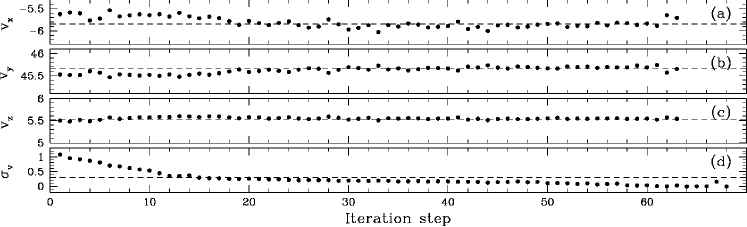
Figure 1: Panels a, b, c: the evolution of the cluster space motion components $v_{x}$, $v_{y}$, and $v_{z}$ (in km s^-1) in the equatorial Cartesian ICRS frame during the rejection of stars in the revised iterative procedure using $\sigma_{v}=0.30$ km s^-1, $\sigma_{\Delta}=0.5$, and a $g$ rejection limit of 9 (§§2.3 and 3.2). The dots show the values of the space motion components at a given iteration step. The dashed lines denote the median values of the space motion components: $(v_{x},v_{y},v_{z})=(-5.84,45.68,5.54)$ km s^-1. Panel d: the evolution of the velocity dispersion $\sigma_{v}$ during the rejection of stars in the unrevised procedure using a $g$ rejection limit of 9 (§§2.2 and 3.1). The dots show the median values of the velocity dispersion at a given iteration step. The discontinuity of the slope of the relation exhibited by the dots around step $\sim$12 coincides with the physical (one-dimensional) velocity dispersion of the Hyades ($\sim$$0.30$ km s^-1; dashed line).

A wealth of ground-based radial velocity information was accumulated for the Hyades over the last century. The cluster has an extent on the sky that is large enough to allow an accurate derivation of its three-dimensional space motion based on proper motion data exclusively (e.g., de Bruijne 1999a, b; Hoogerwerf & Aguilar 1999). We nonetheless decided to modify the maximum likelihood procedure (§2.2) so as to enforce global consistency between the maximum likelihood estimate of the radial component of the cluster space motion and the spectroscopic radial velocity data as a set. Therefore, we multiplied the astrometric likelihood merit function ${\cal L}$ (eq. 6 in B99b) by a radial velocity penalty factor:

$${\cal L}\quad\longrightarrow\quad{\cal L}\cdot\exp{\left({{\Delta^{2}}\over{2\leavevmode\nobreak\ \sigma_{\Delta}^{2}}}\right)},$$ (2)

where $\Delta$ is the median value of $(v_{\rm rad}-v_{\rm rad,pred})/$ $({\sigma_{v_{\rm rad}}^{2}+\sigma_{v}^{2}})^{1/2}$, computed over all stars with a (reliable) radial velocity (§3.2), where $v_{\rm rad,pred}=v_{x}\cos\alpha\cos\delta+v_{y}\sin\alpha\cos\delta+v_{z}\sin\delta$, and $(\alpha,\delta)$ denote the equatorial coordinates of a star. The quantity $\sigma_{\Delta}$ is the allowed inconsistency in $\Delta$. We choose $\sigma_{\Delta}=0.5$, which corresponds to $\sim$$0.25$ km s^-1 when expressed in terms of the median effective radial velocity uncertainty $(\sigma_{v_{\rm rad}}^{2}+\sigma_{v}^{2})^{1/2}\sim 0.50$ km s^-1 (§3.2).

In order to work around the $\sigma_{v}$ bias mentioned in §2.2, we decided to introduce a second modification of the original procedure. This change involves the decoupling of the determination of the cluster motion plus velocity dispersion (§3) from the determination of the secular parallaxes and goodness-of-fit parameters $g$ given the cluster velocity and dispersion (§5; cf. Narayanan & Gould 1999a, b). We thus reduce the dimensionality of the problem from $3+1+n$ to $n$ (cf. §3). However, the $n$-dimensional maximum likelihood problem of finding $n$ secular parallaxes and goodness-of-fit parameters $g$ for a given space motion and velocity dispersion simplifies directly to $n$ independent one-dimensional problems (§2 in B99b). This leads to three additional advantages: (1) it reduces the computational complexity of the problem; (2) it allows an a posteriori decision on the $g$ rejection limit (§2.2); and (3) it allows a treatment on the same footing of stars lacking trigonometric parallax information, such as Hyades selected from the Tycho–2 catalogue (§4.3). In practice, the analysis of such stars only requires the reduction of the dimensionality of the vector of observables ${\mathbf{a}}_{\rm Hip}$ and the corresponding vector ${\mathbf{c}}$ and matrices C_Hip and D from 3 to 2 and $3\times 3$ to $2\times 2$, respectively, through suppression of the first component (see §2 in B99b).

3 Space motion and velocity dispersion

The procedure outlined in §§2.2–2.3 is based on two basic assumptions, namely that (1) the cluster velocity field is known accurately, and (2) the astrometric measurements of the stars correctly reflect their true space motions. Assumption (2) can be safely met by excluding from the analysis (close) multiple systems, spectroscopic binaries, etc. (§4.3). Assumption (1) requires a careful analysis, to which we will return in §6.4. For the moment, it suffices to say that there exist neither conclusive observational evidence nor theoretical predictions that the velocity field of, at least the central region of, the Hyades cluster is non-Gaussian with an anisotropic velocity dispersion.

We opt to define the space motion and velocity dispersion of the Hyades based on a well-defined set of secure members. P98 used the Hipparcos positions, parallaxes, and proper motions, complemented with ground-based radial velocities if available, to derive velocities for individual stars in order to establish membership based on the assumption of a common space motion. P98 identified 218 candidate members, all of which are listed in their table 2 (i.e., column (x) is ‘1’ or ‘?’). We take these stars, and exclude all objects without radial velocity information (i.e., column (p) is ‘$\ast$’) and all (candidate) close binaries (i.e., either column (s) is ‘SB’ (spectroscopic binary) or column (u) is one of ‘G O V X S’; see ESA 1997 for the definition of the Hipparcos astrometric multiplicity fields H59 and H61). This leaves 131 secure single members with high-quality astrometric and radial velocity information^,.

Table 1: Comparison of the Hyades space motion of different studies: this study ([$\sigma_{v}$, $\sigma_{\Delta}$], where $\sigma_{v}=0.20,0.30$, or $0.40$ km s^-1 and $\sigma_{\Delta}=0.1$ or $0.5$; the default is [0.30, 0.50]), Perryman et al. (1998; P98 [134/180] for the 134/180 stars within 10/20 pc of the cluster center), Narayanan & Gould (1999a; NG99a), Dravins et al. (1997; D97), and Lindegren et al. (2000; LMD00). The components of the cluster space motion ${\mathbf{v}}$ in the equatorial Cartesian ICRS coordinate system are $v_{x}$, $v_{y}$, and $v_{z}$ (in km s^-1). The coordinate system $(v_{r},v_{\perp},v_{\parallel})$ is described in §3.2. The convergent point $(\alpha,\delta)_{\rm cp}$ is given in equatorial coordinates (in the ICRS system in degrees). The Hyades convergent point coordinates are strongly correlated; a typical value for the correlation coefficient $\rho$ between $\alpha_{\rm cp}$ and $\delta_{\rm cp}$ is $\rho\sim-0.8$ (§4.1 and figure 4 in de Bruijne 1999a).

Study	$v_{x}$	$\sigma_{v_{x}}$	$v_{y}$	$\sigma_{v_{y}}$	$v_{z}$	$\sigma_{v_{z}}$	$v_{r}$	$v_{\perp}$	$v_{\parallel}$	$\alpha_{\rm cp}$	$\delta_{\rm cp}$
$[0.30,0.5]$	$-5.84$	0.26	45.68	0.11	5.54	0.07	39.48	$0.00$	24.35	97.29	6.86
$[0.30,0.1]$	$-5.74$	0.10	45.67	0.08	5.58	0.04	39.52	$-0.00$	24.25	97.16	6.91
$[0.20,0.5]$	$-5.77$	0.10	45.64	0.05	5.59	0.07	39.49	$-0.03$	24.25	97.21	6.93
$[0.40,0.5]$	$-5.99$	0.18	45.73	0.09	5.52	0.05	39.46	$-0.03$	24.50	97.46	6.83
P98 [134]	$-6.28$	0.20	45.19	0.20	5.31	0.20	38.82	$-0.02$	24.56	97.91	6.66
P98 [180]	$-6.32$	0.20	45.24	0.20	5.30	0.20	38.84	$-0.02$	24.62	97.96	6.61
NG99a	$-5.70$	0.20	45.62	0.11	5.65	0.08	39.51	$-0.06$	24.17	97.12	7.01
D97	$-6.07$	0.13	45.77	0.36	5.53	0.11	39.47	$-0.06$	24.59	97.55	6.83
LMD00	$-5.90$	0.13	45.65	0.34	5.56	0.10	39.44	$-0.05$	24.38	97.36	6.89

3.1 Velocity dispersion

We start the unrevised procedure (§2.2) for the above-described sample of 131 stars using a $g$ rejection limit of 9. Figure 1 (panel d) shows the evolution of the maximum likelihood value derived for $\sigma_{v}$ while rejecting stars. The estimated velocity dispersion decreases rapidly, more-or-less linearly, from $\sim$1 km s^-1 initially to $\sim$$0.30$ km s^-1 in the first $\sim$11 steps. Previous studies of the Hyades cluster show that its physical (one-dimensional) velocity dispersion is $\sim$$0.30$ km s^-1 (Gunn et al. 1988: $0.23\pm 0.05$ km s^-1; Zhao & Chen 1994: $0.37\pm 0.04$ km s^-1; Dravins et al. 1997: $0.25\pm 0.04$ km s^-1; P98: 0.20–0.40 km s^-1; Narayanan & Gould 1999a, b: $0.32\pm 0.04$ km s^-1; Lindegren et al. 2000: $0.31\pm 0.02$ km s^-1; Makarov et al. 2000: $\sim$0.32 km s^-1). From step $\sim$12 onwards, the maximum likelihood dispersion estimate decreases, again more-or-less linearly but much more gradually, to $\sim$0 km s^-1 in step $\sim$60–70. Not surprisingly, the corresponding evolution of the space motion shows an unwanted trend beyond step $\sim$12 (not shown): the unrevised method is forced to search for a maximum likelihood solution which has a velocity dispersion that is smaller than the physical value.

Given the Hyades space motion (or convergent point; §3.2), a semi-independent estimate of the internal velocity dispersion $\sigma_{v}$ can be derived through a so-called $\mu_{\perp}$-component analysis (§20 in Blaauw 1946; §7.2 in P98; §4.2 in B99b; Lindegren et al. 2000). The $\mu_{\perp}$ proper motion components are directed perpendicular to the great circle joining a star and the apex, and as such, by definition, exclusively represent peculiar motions ($\Delta_{v,\perp}$; one-dimensional, in km s^-1) and observational errors ($\Delta_{\mu_{\perp}}$; in mas yr^-1):

$$\mu_{\perp}=A^{-1}\pi\Delta_{v,\perp}+\Delta_{\mu_{\perp}}\Longrightarrow\overline{\mu_{\perp}^{2}}=\overline{(A^{-1}\pi\Delta_{v,\perp})^{2}}+\overline{\Delta_{\mu_{\perp}}^{2}},$$ (3)

where the step follows from the statistical independence of the peculiar motions and the observed proper motion errors. Upon using $\pi=21.58$ mas ($D=46.34$ pc; P98), and calculating $\mu_{\perp}$ and $\Delta_{\mu_{\perp}}$ from the Hipparcos positions and proper motions using the maximum likelihood apex $(\alpha_{\rm cp},\delta_{\rm cp})=(97\aas@@fstack{\circ}29,6\aas@@fstack{\circ}86)$ (Table 1; §3.2), it follows that $({\overline{\Delta_{v,\perp}^{2}}})^{1/2}\sim 0.20$–$0.40$ km s^-1, where the precise value of this quantity depends on the details of the selection and subdivision of the stellar sample (Table 2). The abovementioned range is consistent with our assumed value of $0.30$ km s^-1. We therefore decided to take $\sigma_{v}=0.30$ km s^-1 fixed in the remainder of this study, i.e., we reduce the dimensionality of the problem from $3+1+n$ to $3+n$ (§2.3).

3.2 Space motion

Our next step is to start the revised procedure (§2.3) for the same sample of 131 stars, but take $\sigma_{v}=0.30$ km s^-1 and $\sigma_{\Delta}=0.5$. We exclude multiple systems without a known systemic (or center-of-mass or $\gamma$-) velocity, as well as objects with a variable radial velocity, in the calculation of the penalty factor (eq. 2; i.e., all stars with a #-sign preceding column (q) in P98’s table 2). Figure 1 shows the evolution of the maximum likelihood estimates of the space motion components while rejecting stars; we derive $(v_{x},v_{y},v_{z})=(-5.84\pm 0.26,45.68\pm 0.11,5.54\pm 0.07)$ km s^-1. Table 1 shows the results of varying $\sigma_{\Delta}$ and $\sigma_{v}$. Changing $\sigma_{\Delta}$, for example, from 0.5 to 0.1 at fixed $\sigma_{v}=0.30$ km s^-1 yields a set of secular parallaxes (§5) which differ systematically in the sense $\langle\pi_{{\rm sec},\sigma_{\Delta}=0.1}-\pi_{{\rm sec},\sigma_{\Delta}=0.5}\rangle\sim+0.08$ mas, independent of visual magnitude. We take $(v_{x},v_{y},v_{z})=(-5.84,45.68,5.54)$ km s^-1 fixed in the remainder of this study, i.e., we reduce the dimensionality of the problem, now from $3+n$ to $n$.

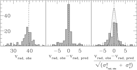
Figure 2: Observed ($v_{\rm rad,obs}$) and predicted ($v_{\rm rad,pred}$; §2.3) radial velocities for 131 secure members (§3). Left: distribution of observed radial velocities; the dashed line denotes the radial component of the Hyades cluster motion derived in this study ($39.48$ km s^-1) using $\sigma_{v}=0.30$ km s^-1 and $\sigma_{\Delta}=0.5$ ([0.30, 0.5] in Table 1). The spread and skewness of the distribution are caused by the perspective effect. Middle: distribution of observed minus predicted radial velocities; 71/60 stars have negative/positive $v_{\rm rad,obs}-v_{\rm rad,pred}$. Right: normalized distribution of observed minus predicted radial velocities, taking into account a velocity dispersion of $\sigma_{v}=0.30$ km s^-1. The black curve is a properly scaled zero-mean unit-variance Gaussian; the mismatch between the observations and prediction can be due to non-members and/or undetected close binaries, an underestimated velocity dispersion, underestimated radial velocity errors, or a combination of these effects (§3.2). Five stars fall outside the plotted range.

Table 1 compares the space motions found by us with results derived by P98, Dravins et al. (1997), Narayanan & Gould (1999a), and Lindegren et al. (2000) from Hipparcos data. We refrain from comparing our values to pre-Hipparcos results (e.g., Schwan 1991; Zhao & Chen 1994; Cooke & Eichhorn 1997), as these are (possibly) influenced by fundamental uncertainties in the pre-Hipparcos proper motion reference frames (the Hipparcos positions and proper motions are absolute, and are given in the Hipparcos ICRS inertial reference frame; cf. §4 in P98). Table 1 also compares the different space motions in the $(v_{r},v_{\perp},v_{\parallel})$ coordinate system, which is oriented such that the $v_{r}$-axis is along the radial direction of the cluster center, which is (arbitrarily) defined as $(\alpha,\delta)_{\rm center}=(4^{\rm h}\,26^{\prime}\,32^{\prime\prime},17^{\circ}\!{\leavevmode\nobreak\ }13{\aas@@fstack{\prime}}3)$ (J2000.0), the $v_{\perp}$-axis is along the direction perpendicular to the cluster proper motion in the plane of the sky, and the $v_{\parallel}$-axis is parallel to the cluster proper motion in the plane of the sky. We conclude that our space motion is consistent with the values derived by Dravins et al., P98, Narayanan & Gould, and Lindegren et al.; our radial motion agrees very well with the Dravins et al., Narayanan & Gould, and Lindegren et al. values, whereas our tangential motion perfectly agrees with Lindegren et al. and lies between the Narayanan & Gould value on the one hand and the P98 and Dravins et al. values on the other hand. The radial components of the P98 space motions ($38.82$–$38.84$ km s^-1) deviate significantly (at the level of $\sim$0.70 km s^-1) from all other values in Table 1 (cf. §4.2 in Narayanan & Gould 1999a). Unfortunately, the mean spectroscopically determined radial velocity of the Hyades cluster is not well defined; Detweiler et al. (1984), for example, find $39.1\pm 0.2$ km s^-1, but their table 1 gives an overview of previous determinations which show a discouragingly large spread (cf. Gunn et al. 1988). Figure 2 shows, for the 131 secure single members, the distribution of observed radial velocities (left), the distribution of observed minus predicted radial velocities (§2.3) given the cluster space motion (middle), and the properly normalized distribution of observed minus predicted radial velocities (right; taking into account a velocity dispersion of $\sigma_{v}=0.30$ km s^-1). The distribution of observed radial velocities is not symmetric but skewed towards lower $v_{\rm rad,obs}$ values; the median $v_{\rm rad,obs}$ value ($38.60$ km s^-1) is $0.66$ km s^-1 larger than the straight mean of the observed $v_{\rm rad,obs}$ values ($37.94$ km s^-1). The large spread and skewness in the distribution of observed radial velocities are caused by the perspective effect, which is significant for the Hyades due to its large extent on the sky (§1). The perspective effect has been removed in the middle and right panels of Figure 2. The middle panel shows that the radial component of our space motion ($39.48$ km s^-1) yields an acceptable $v_{\rm rad,obs}-v_{\rm rad,pred}$ distribution. The deviation between the predicted zero-mean unit-variance Gaussian and the observed histogram in the right panel is possibly caused by (1) the presence of a few non-members (and possibly some not-detected close binaries), (2) a slightly underestimated cluster velocity dispersion, and/or (3) underestimated $v_{\rm rad,obs}$ errors. The histogram and Gaussian prediction would agree, given the $v_{\rm rad,obs}$ errors, if $\sigma_{v}$ is increased to $\sim$0.80–0.90 km s^-1, or, given $\sigma_{v}=0.30$ km s^-1, if the individual random $v_{\rm rad,obs}$ errors are increased by an amount of $\sim$0.50–0.60 km s^-1. While the first possibility seems highly unlikely (§3.1; cf. Gunn et al. 1988), the required ‘extra radial velocity uncertainty’ is not unreasonable, given it is of the same order of magnitude as the (poorly determined) non-physical zero-point shifts usually adopted in radial velocity studies (e.g., Gunn et al. 1988; cf. §§3.2 and 7.2 in P98).

4 Membership

Having determined the Hyades space motion and velocity dispersion, we are in a position to discuss membership.

4.1 Hipparcos: Perryman et al. (1998) candidates

Table 2: Statistics of the $\mu_{\perp}$ proper motion components for the 63 brightest (${\rm spectral\leavevmode\nobreak\ type=SpT}\leq{\rm G5}$) high-fidelity ($g\equiv g_{\rm Hip}\leq 9$; §5) single P98 members (column (s) in P98’s table 2 is not ‘SB’), using $(\alpha_{\rm cp},\delta_{\rm cp})=(97\aas@@fstack{\circ}29,6\aas@@fstack{\circ}86)$ (see eq. 3 and §3.1). Hyades main sequence members with spectral types later than $\sim$G5 have modest Hipparcos proper motion accuracies due to their faint magnitudes ($V\mathrel{{\hbox to0.0pt{\lower 3.0pt\hbox{$\sim$}\hss}}\raise 2.0pt\hbox{$>$}}8.5$ mag; e.g., figure 1 in Hoogerwerf 2000). Results are tabulated for four ranges in spectral type ($n$ stars from ${\rm SpT}_{-}$ trough ${\rm SpT}_{+}$); the spectral-type averaged value of $({\overline{\Delta_{v,\perp}^{2}}})^{1/2}$   for these 63 stars is $\sim$0.25 km s^-1.

${\rm SpT}_{-}$	${\rm SpT}_{+}$	$n$	$(\overline{{\mu_{\perp}^{2}}})^{1/2}$	$(\overline{{\Delta_{\mu_{\perp}}^{2}}})^{1/2}$	$({\overline{\Delta_{v,\perp}^{2}}})^{1/2}$
			mas	mas	km s-1
A2	F0	16	1.35	0.89	0.23
F0	F5	16	1.71	0.88	0.31
F5	F8	16	1.33	0.96	0.20
F9	G5	15	1.71	1.13	0.28

The Hipparcos Catalogue contains 118 218 entries which are homogeneously distributed over the sky. The catalogue is complete to $V\sim 7.3$ mag, and has a limiting magnitude of $V\sim 12.4$ mag. In the case of the Hyades, special care was taken to optimize the number of candidate members in the Hipparcos target list. As a result, the Hipparcos Input Catalogue (Turon et al. 1992) contains $\sim$240 candidate Hyades members in the field $2^{\rm h}\,15^{\rm m}<\alpha<6^{\rm h}\,5^{\rm m}$ and $-2^{\circ}\!<\delta<35^{\circ}\!$ (§3.1 in P98). P98 considered all 5 490 Hipparcos entries in this field for membership, and ended up with 218 members. The P98 member selection is generous: only very few genuine members, contained in both the Hipparcos Catalogue and the selected field on the sky, have probably not been selected, whereas a number of field stars (interlopers) are likely to be present in their list. P98 distinguish members (197 stars) and possible members (21 stars); the latter do not have measured radial velocities (column (x) = ‘?’ in their table 2).

P98 divide the Hyades into four components ($r$ is the three-dimensional distance to the cluster center): (1) a spherical ‘core’ with a $2.7$ pc radius and a half-mass radius of $5.7$ pc; (2) a ‘corona’ extending out to the tidal radius $r_{\rm t}\sim 10\leavevmode\nobreak\ {\rm pc}$ (134 stars in core and corona); (3) a ‘halo’ consisting of stars with $r_{\rm t}\la r\la 2r_{\rm t}$ which are still dynamically bound to the cluster (45 stars; e.g., Pels et al. 1975); and (4) a ‘moving group population’ of stars, possibly former members, with $r\ga 2r_{\rm t}$ which have similar kinematics to the bound members in the central parts of the cluster (39 stars; e.g., Asiain et al. 1999; cf. §7 in P98).

The fact that P98 restricted their search to a pre-defined field on the sky limits knowledge on and completeness of membership, especially in the outer regions of the cluster: the 10 pc tidal radius translates to a cluster diameter of $\sim$$25^{\circ}\!$, whereas the P98 field measures $57\aas@@fstack{\circ}5$ in $\alpha$ and $37\aas@@fstack{\circ}0$ in $\delta$. Although this problem seems minor at first sight, suggesting a solution in the form of simply searching the entire Hipparcos Catalogue for additional (moving group) members, it is daunting in practice: thousands of Hipparcos stars all over the sky have proper motions directed towards the Hyades convergent point (§4.2 in de Bruijne 1999a). Whereas this in principle means that these stars, in projection at least, are ‘co-moving’ with the Hyades, the identification of physical members of a moving group (or ‘supercluster’) population is not trivial, and requires additional observational data (cf. §§7–8 and table 6 in P98; §6.4.2). We therefore restrict ourselves to the P98 field (§4.2). Section 4.3 discusses the possibility to extend membership down to fainter magnitudes using the Tycho–2 astrometric catalogue.

4.2 Hipparcos: additional candidates

De Bruijne (1999a) and Hoogerwerf & Aguilar (1999) re-analyzed Hyades membership, based on the refurbished convergent point and Spaghetti method. These studies used Hipparcos data but excluded radial velocity information. The convergent point method uses proper motion data only, confirms membership for 203 of the 218 P98 members (cf. Table LABEL:tab:data_1), and selects $12$ new candidates within 20 pc of the cluster center. The Spaghetti method, using proper motion and parallax data, selects six new candidate members, three of which are in common with the $12$ proper motion candidates mentioned above. The Spaghetti method does not confirm 56 P98 members (cf. Table LABEL:tab:data_1); however, 49 of these are low-probability (i.e., ‘1–3$\sigma$’) P98 members. Table 7 lists the 15 new candidates. We defer the discussion of these stars to §5.2.

4.3 Tycho–2: bright binaries and faint candidates

The Tycho(–1) Catalogue (ESA 1997), which is based on measurements of Hipparcos’ starmapper, contains astrometric data for $\sim$1 million stellar systems with a $\sim$10–20 times smaller precision than Hipparcos. Its completeness limit is $V\sim 10.5$ mag. Despite the ‘inferior astrometric precision’, the Tycho positions as a set are superior to similar measurements in any other catalogue of comparable size. The Tycho measurements (median epoch 1991.25) have therefore been used as second epoch material in the construction of a long time-baseline proper motion project, culminating in the Tycho–2 catalogue (Høg et al. 2000a, b; cf. Urban et al. 1998a; Kuzmin et al. 1999). This project uses the Astrographic Catalogue positions, as well as data from 143 other ground-based astrometric catalogues, as first epoch material (median epoch $\sim$1904). The Astrographic Catalogue (Débarbat et al. 1988; Urban et al. 1998b) was part of the ‘Carte du Ciel’ project, which envisaged the imaging of the entire sky on 22 660 overlapping photographic plates by 20 observatories in different ‘declination zones’. The Tycho–2 catalogue contains absolute proper motions in the Hipparcos ICRS frame for $\sim$2.5 million stars with a median error of $\sim$2.5 mas yr^-1. Its completeness limit is $V\sim 11.0$ mag. Tycho–2 contains proper motions for 208 of the 218 P98 candidates; the entries HIP 20440, 20995, and 23205 are (photometrically) resolved binaries in Tycho–2.

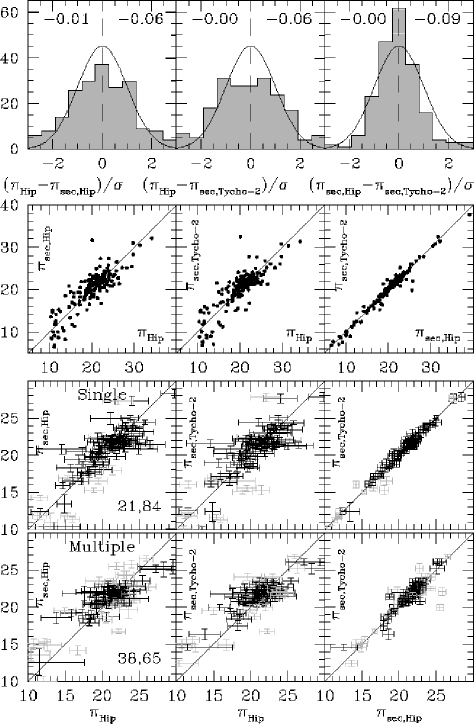
Figure 3: First and second row: the 208 entries which have Hipparcos trigonometric ($\pi_{\rm Hip}$), Hipparcos secular ($\pi_{\rm sec,Hip}$), and Tycho–2 secular ($\pi_{\rm sec,Tycho-2}$) parallaxes (in mas). The top row shows properly normalized difference distributions for $\pi_{\rm Hip}-\pi_{\rm sec,Hip}$ (column 1), $\pi_{\rm Hip}-\pi_{\rm sec,Tycho-2}$ (column 2), and $\pi_{\rm sec,Hip}-\pi_{\rm sec,Tycho-2}$ (column 3). The black curves are zero-mean unit-variance Gaussian distributions. The numbers in the top of each top panel denote the mean (left) and median (right) of the plotted difference. The second row compares the different parallaxes. Third and fourth row: trigonometric and secular parallaxes, and their random errors (§5.4), for the same stars. The third row compares the different parallaxes for single stars, while the bottom row shows multiple stars (i.e., either column (s) in P98’s table 2 is ‘SB’ or ‘RV’, column (t) is ‘H’, ‘I’, or ‘M’, or column (u) is one of ‘C G O V X S’). Black symbols have $g_{\rm Hip}\leq 9$; gray symbols have $g_{\rm Hip}>9$. The numbers in the left panels indicate the relevant numbers of stars (gray, black). Stars having large goodness-of-fit parameters $g_{\rm Hip}$ are $\sim$2 times more likely multiple than low-$g_{\rm Hip}$ stars (cf. §3).

The Tycho–2 proper motions can be used in two ways. First, as a result of the $\sim$4 year time baseline over which Hipparcos obtained its astrometric data, the proper motions of some multiple systems do not properly reflect their true systemic motions as a result of unrecognized orbital motion (e.g., de Zeeuw et al. 1999; Wielen et al. 1999, 2000; these systems are called ‘$\Delta\mu$ binaries’). As the long time-baseline Tycho–2 proper motions suffer from this effect to a much smaller extent, they sometimes significantly better represent the true motion of an object than the Hipparcos measurements do. Second, the Tycho–2 catalogue can in principle be used to provide membership information for stars beyond the Hipparcos completeness limit, i.e., in the range $7.3\la V\la 12.4$ mag (the Tycho–2 catalogue contains $\sim$90,000 stars in P98’s Hyades field). The search for new (faint) members is, however, non-trivial. The Hipparcos Catalogue in the field of the Hyades is already relatively complete in terms of (known) members of the cluster (cf. figure 2 and §3.1 in P98), so that the majority of new members is necessarily quite faint ($V\ga 10.0$ mag). Moreover, most of the Tycho–2 entries have no known radial velocity and/or parallax (although some stars in the Tycho–2 catalogue have Tycho parallax measurements, the typical associated random errors for Hyades fainter than $V\sim 7.3$ mag are similar in size or larger than the expected parallaxes themselves, $\pi\sim 22$ mas). We therefore cannot select (faint) Tycho–2 Hyades members along the lines set out by P98, but must, e.g., follow Hoogerwerf’s (2000) method instead. This method, which is based on a convergent point method, selects (faint) stars which (1) are consistent with a given convergent point and the two-dimensional proper motion distribution of a given set of (bright) Hipparcos members, and (2) follow a given main sequence. However, the resulting list of candidate members contains hundreds of falsely identified objects (interlopers), especially in the faint magnitude regime (e.g., Hoogerwerf 2000; cf. de Bruijne 1999a). Reliable suppression of these stars requires at least (yet unavailable) radial velocity and/or parallax data. We therefore refrain from pursuing this route further in this paper.

5 Secular parallaxes

Table 3: Hipparcos and Tycho–2 secular parallaxes, and associated goodness-of-fit parameters $g_{\rm Hip}$ and $g_{\rm Tycho-2}$, for the binaries which have both trigonometric (ESA 1997) and orbital parallaxes (Torres et al. 1997a, b, c).

HIP	TYC	$\pi_{\rm Hip}$	$\pi_{\rm sec,Hip}$	$\pi_{\rm sec,Tycho-2}$	$\pi_{\rm orb}$	$g_{\rm Hip}$	$g_{\rm Tycho-2}$
		mas	mas	mas	mas
20087a	1276 1622 1	$18.25\pm 0.82$	$18.31\pm 0.69$	$18.70\pm 0.29$	$17.92\pm 0.58$	0.19	0.00
20661b	1265 1171 1	$21.47\pm 0.97$	$21.29\pm 0.37$	$21.08\pm 0.38$	$21.44\pm 0.67$	7.20	0.00
20894c	1265 1172 1	$21.89\pm 0.83$	$22.24\pm 0.36$	$22.35\pm 0.36$	$21.22\pm 0.76$	0.26	0.22

^a: $\pi_{\rm trigonometric}=19.4\pm 1.1$ mas (Gatewood et al. 1992) and $\pi_{\rm trigonometric}=18.23\pm 0.86$ mas (Söderhjelm 1999).
^b: $\pi_{\rm trigonometric}=22.1\pm 1.1$ mas (Söderhjelm 1999).
^c: See §§10.3 and B.3 for a discussion of this system.

We now determine secular parallaxes for the 218 P98 members and the 15 new candidates discussed in §4, using the space motion and velocity dispersion found in §3 ($v_{x},v_{y},v_{z},\sigma_{v}=-5.84,45.68,5.54,0.30$ km s^-1) as constants (§2.3). This provides, for each proper motion (either Hipparcos or Tycho–2), a secular parallax ($\pi_{\rm sec,Hip}$ or $\pi_{\rm sec,Tycho-2}$) and an associated random error ($\sigma_{\pi,{\rm sec,Hip}}$ or $\sigma_{\pi,{\rm sec,Tycho-2}}$; §5.4) and goodness-of-fit parameter ($g_{\rm Hip}$ or $g_{\rm Tycho-2}$; Appendix A). As the Hipparcos and Tycho–2 proper motions are independent measurements, the corresponding secular parallaxes can in principle be averaged, taking the errors into account as weighting factors. It is, however, less clear how to incorporate the goodness-of-fit parameters $g_{\rm Hip}$ and $g_{\rm Tycho-2}$ in the averaging process. We therefore provide both secular parallaxes for all stars and refrain from giving any average value.

5.1 Hipparcos: Perryman et al. (1998) candidates

Figure 3 shows a global comparison between the different sets of parallaxes. The mean and/or median Hipparcos parallax is equal to the mean and/or median secular parallax (either Hipparcos or Tycho–2) to within $\la$0.10 mas. This implies that the secular parallaxes are reliable and do not suffer from a significant systematic component (cf. §6). This conclusion is supported by Table 3, which compares trigonometric and secular parallaxes for three Hyades binaries which also have orbital parallaxes.

The goodness-of-fit parameter $g_{\rm Hip}$ allows a natural division between high-fidelity kinematic members ($g_{\rm Hip}\leq 9$) and kinematically deviant stars ($g_{\rm Hip}>9$; §2.2; cf. Figure 5). The latter are not necessarily non-members, but can also be (close) multiple stars for which the Hipparcos proper motions do not properly reflect the center-of-mass motion (§4.3). Fifty of the 197 P98 members with known radial velocities have $g_{\rm Hip}>9$, which leaves a number of high-fidelity members similar to that found by Dravins et al. (1997; 133 stars), Madsen (1999; 136 stars), and Narayanan & Gould (1999b; 132 stars)(cf. table 3 in Lindegren et al. 2000). Fourteen of the 21 possible P98 members (column (x) = ’?’ in their table 2) have $g_{\rm Hip}>9$. These stars do not have measured radial velocities (§4.1), and P98 membership is based on proper motion data only. All but one of these stars are rejected as Hyades members by de Bruijne (1999a) and/or Hoogerwerf & Aguilar (1999; Table LABEL:tab:data_1; cf. §4.2). The 14 suspect secular parallaxes thus most likely indicate these objects are non-members.

5.2 Hipparcos: additional candidates

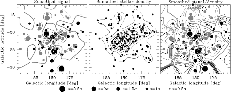
Figure 4: Left: the trigonometric-minus-secular parallax difference field $s(\ell,b)$ (eq. 4), smoothed using the Gaussian kernel $G(\ell,b)$ (eq. 5) with smoothing length $\sigma_{\rm s}=1^{\circ}\!$. Solid contours correspond to $s\geq 0$; dotted contours correspond to $s<0$; gray contours denote $s=0$. Heavy/light contours are spaced by $1.0$/$0.25$. The dots indicate the positions of 127 Hyades with non-suspect secular parallaxes ($g_{\rm Hip}\leq 9$). Black symbols have $s\geq 0$ (60 stars), while gray symbols have $s<0$ (67 stars). The symbol sizes correspond linearly to the strength of the signal $s$ (larger symbols denote larger $|s|$; see legend). Middle: as left panel, but for the projected stellar number density $\rho(\ell,b)\equiv\delta_{\rm D}(\ell,b)$. The lowest contour level equals $0.25$ star ${\rm deg}^{-2}$. Right: as left panel, but for the signal $s(\ell,b)$ divided by the density $\rho(\ell,b)$.

Table 7 lists secular parallaxes for the 15 additional candidate members (§4.2). The assumption that these stars share the same space motion as the Hyades cluster (in other words: the assumption of membership) generally results in both high values for the goodness-of-fit parameters $g_{\rm Hip}$ and secular parallaxes which are inconsistent with the trigonometric values. This means these stars are likely non-members (cf. §4.2 in B99b); only three of them (HIP 19757, 21760, and 25730) have $g_{\rm Hip}\leq 9$. In retrospect, especially HIP 19757 is a likely new member: it was selected as candidate both by de Bruijne (1999a) and Hoogerwerf & Aguilar (1999); it has an uncertain trigonometric parallax ($\pi_{\rm Hip}=16.56\pm 4.48$ mas) due to its faint magnitude ($V=11.09$ mag); it has a Hipparcos secular parallax ($\pi_{\rm sec,Hip}=20.19\pm 1.04$ mas; $g_{\rm Hip}=2.67$) which places it at only 7.15 pc from the cluster center; its Hipparcos secular parallax puts it on the Hyades main sequence (§8); and it has an unknown radial velocity.

5.3 Tycho–2: faint candidates

The ‘Base de Données des Amas ouverts’ database (BDA; http://obswww.unige.ch/webda/webda.html) contains 23 photometric Hyades which are not contained in the Hipparcos Catalogue but which were observed by Tycho (cf. §3.1 and figure 2 in P98). The Tycho–2 secular parallaxes of most of these stars lie between 18 and 22 mas, indicating they are located at the same distance as the bulk of the bright Hyades. Only four of them have $g_{\rm Tycho-2}>9$. Most of these stars are thus likely members. We discuss their HR diagram positions in §8.

5.4 Random secular parallax errors

Table LABEL:tab:data_1 contains random secular parallax errors resulting from both uncertainties in the underlying proper motions and the internal velocity dispersion in the cluster ($\sigma_{v}=0.30$ km s^-1; §4.1 in B99b). Hipparcos/Tycho–2 secular parallax errors for Hyades are on average a factor $\sim$3.0 smaller than the corresponding Hipparcos trigonometric parallax errors.

6 Systematic secular parallax errors?

Although the secular parallaxes derived in §5 have small random errors, they might suffer from significant systematic errors. In this section, we investigate the influences of the maximum likelihood method, the uncertainty of the tangential component of the cluster space motion (§6.1), the correlated Hipparcos measurements (§6.2), as well as possible unmodelled patterns in the velocity field of the Hyades (§6.4). Section 6.5 summarizes our results.

6.1 Cluster space motion

Extensive Monte Carlo tests of the maximum likelihood procedure (§§2.2–2.3) show that, given the correct cluster space motion, the method is not expected to yield systematic secular parallax errors larger than a few hundredths of a mas (e.g., §§3.2.2.1 and 3.2.2.3, table 3, and figure 5 in B99b). It is possible, though, that a systematic error is introduced through the use of an incorrect value for the tangential component of the cluster space motion ($v_{\parallel}$; §3.2). We estimate $\sigma_{v_{\parallel}}\sim 0.15$ km s^-1 from Table 1. This uncertainty gives rise to maximum systematic secular parallax errors of $\sim$0.14 mas ($\sigma_{v_{\parallel}}=0.30$ km s^-1 gives 0.28 mas; see §4.2 in B99b and use $v_{\parallel}=24.35$ km s^-1, $\overline{\mu}=111.0$ mas yr^-1, $\sigma_{\overline{\mu}}=0.15$ mas yr^-1, and $\overline{\pi_{\rm Hip}}=1000.0/45.0$ mas). This value compares favorably to typical random secular parallax errors for Hyades ($\sim$$0.50$ mas; Table LABEL:tab:data_1). It is, nonetheless, desirable to obtain a more precise estimate of the tangential component of the cluster space motion. This requires a better knowledge of the associated radial space motion component and internal velocity dispersion and/or more precise proper motion measurements (§11).

6.2 Hipparcos correlations on small angular scales

The Hipparcos Catalogue contains absolute astrometric data. Absolute in this sense should be interpreted as lacking global systematic errors at the $\sim$0.10 mas (yr^-1) level or larger (ESA 1997; cf. Narayanan & Gould 1999a, who quote an upper limit of $0.47$ mas for the Hyades field). However, the measurement principle of the satellite does allow for the existence of correlated astrometric parameters on small angular scales ($\sim$$1^{\circ}\!$–$3^{\circ}\!$; e.g., Lindegren 1989; ESA 1997, Vol. 3, p. 323 and 369). These correlations have been suggested to be responsible for the so-called ‘Pleiades anomaly’, i.e., the fact that the mean distance of the Pleiades cluster as derived from the mean Hipparcos trigonometric parallax differs from the value derived from stellar evolutionary modelling (Pinsonneault et al. 1998; but see, e.g., Robichon et al. 1999; van Leeuwen 1999).

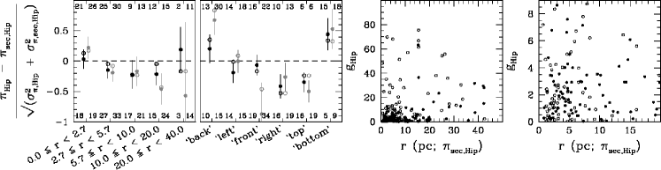
Figure 5: Left two panels: normalized difference between Hipparcos trigonometric and secular parallaxes for the 218 P98 members as function of location in the cluster. The left panel shows a spatial division according to $r$ (the three-dimensional distance to the cluster center using Hipparcos secular parallaxes) in five spherical annuli (from center to core radius [2.7 pc] to half-mass radius [5.7 pc] to tidal radius [10 pc] to two tidal radii [20 pc] to 40 pc). The cluster center is $(b_{u},b_{v},b_{w})=(-43.37,0.40,-17.46)$ pc in Galactic Cartesian coordinates (cf. table 3 in P98). The right panel shows a spatial division according to the six equal-volume pyramids (§6.3; orientation in Galactic coordinates). Black/gray symbols show results for stars with $g_{\rm Hip}\leq 9/\infty$. Filled symbols and vertical lines denote mean and standard deviation ($\pm$1$\sigma$ uncertainty), while open symbols denote median values; the numbers in the upper/lower halves of the panels denote the corresponding numbers of stars with $\pi_{\rm Hip}-\pi_{\rm sec,Hip}>$/$\leq 0$. Right two panels: the goodness-of-fit parameter $g_{\rm Hip}$ as function of $r$ (left; 202 stars) and a magnification of this panel for 144 high-fidelity (i.e., low-$g_{\rm Hip}$) members in the central parts of the cluster (right). Open symbols denote multiple stars (i.e., either column (s) in P98’s table 2 is ‘SB’ or ‘RV’, column (t) is ‘H’, ‘I’, or ‘M’, or column (u) is one of ‘C G O V X S’; 103/64 entries in the left/right panel).

The left panel of Figure 4 shows the $1^{\circ}\!$-smoothed error-normalized difference field of the Hipparcos trigonometric minus secular parallaxes for all stars with non-suspect secular parallaxes ($g_{\rm Hip}\leq 9$) in the center of the Hyades cluster ($170\aas@@fstack{\circ}0\leq\ell\leq 190\aas@@fstack{\circ}0$ and $-32\aas@@fstack{\circ}0\leq b\leq-12\aas@@fstack{\circ}0$; $\ell$ and $b$ denote Galactic coordinates). In order to obtain this field, we convolved the sum of the discrete quantity $s$:

$$s=s(\ell,b)\equiv\delta_{\rm D}(\ell,b)\cdot{{\pi_{\rm Hip}-\pi_{\rm sec,Hip}}\over{\sqrt{(}\sigma_{\pi,{\rm Hip}}^{2}+\sigma_{\pi,{\rm sec,Hip}}^{2})}},$$ (4)

where $\delta_{\rm D}$ denotes the two-dimensional Dirac delta function, for each star with the normalized two-dimensional Gaussian smoothing kernel

$$G(\ell,b)\equiv{{1}\over{2\pi\sigma_{\rm s}^{2}}}\cdot\exp\left(-{{1}\over{2}}\left[{{\ell^{2}+b^{2}}\over{\sigma_{\rm s}^{2}}}\right]\right),$$ (5)

where $\sigma_{\rm s}=1^{\circ}\!$ is the smoothing length. The appearance of the difference field depends on the adopted smoothing length, though not very sensitively. Taking a large smoothing length returns a smooth field, whereas a small smoothing length gives a ‘spiky distribution’, reminiscent of the original delta function-type field (eq. 4). Given a Hyad, its closest neighbour on the sky is typically found at an angular separation of $\sim$$0\aas@@fstack{\circ}5$. Our choice of the smoothing length ($1\aas@@fstack{\circ}0$) corresponds to the median value (for all stars) of the median angular separation of the $\sim$3–4 nearest neighbours on the sky. We checked that the smoothed difference field has the same overall appearance when adopting smoothing lengths of $0\aas@@fstack{\circ}5$ or $2\aas@@fstack{\circ}0$.

The smoothed difference field shows several positive and negative peaks with a full-width-at-half-maximum of a few degrees. These peaks can be due to spatially correlated errors in the Hipparcos parallaxes $\pi_{\rm Hip}$ on small angular scales, spatially correlated errors in the Hipparcos secular parallaxes $\pi_{\rm sec,Hip}$ on small angular scales, or both. From the fact that the peaks are not evident in the smoothed difference field of the Hipparcos secular parallaxes and the mean cluster parallax (not shown), whereas they are present in the smoothed difference field of the Hipparcos trigonometric parallaxes and the mean parallax (not shown), we conclude that they are mainly caused by correlated Hipparcos measurements, notably the trigonometric parallaxes (cf. Narayanan & Gould 1999b). As the relative precision of the Hipparcos proper motions is $\sim$5 times higher than the relative precision of the Hipparcos trigonometric parallaxes (cf. §1), the Hipparcos secular parallaxes, which have more-or-less been directly derived from the Hipparcos proper motions, are correlated as well, though with smaller ‘amplitudes’.

The quantity $s$ (eq. 4) denotes, for a given star, the dimensionless significance (in terms of the effective Gaussian standard deviation $\sigma\equiv(\sigma_{\pi,{\rm Hip}}^{2}+\sigma_{\pi,{\rm sec,Hip}}^{2})^{1/2}\sim 1.5$ mas) of the parallax difference $\pi_{\rm Hip}-\pi_{\rm sec,Hip}$. As the smoothing kernel $G$ (eq. 5) is properly normalized to unit area in two dimensions, the smoothed difference field can be interpreted in terms of net significance per square degree. The right panel of Figure 4 shows the corresponding smoothed difference field expressed in terms of net significance per star. This field was obtained by dividing the smoothed signal field by an identically smoothed stellar number density field $\rho(\ell,b)\equiv\delta_{\rm D}(\ell,b)$ (middle panel of Figure 4). The smoothed difference field expressing significance per star also contains patches of size a few degrees with both negative and positive contributions, although there is no large-scale trend (cf. Figure 3). We thus conclude that the Hipparcos trigonometric parallaxes towards the Hyades cluster are spatially correlated over angular scales of a few degrees. The maximum deviations in the central region of the cluster ($\rho\ga 0.5\leavevmode\nobreak\ {\rm star}\leavevmode\nobreak\ {\rm deg}^{-2}$), however, are generally less than $\sim$$0.50$–$0.75\sigma$ per star (i.e., $\la$ $0.75$–$1.00$ mas). The signal in the outer parts of the cluster is statistically non-interpretable as it is severely influenced by the contributions of individual stars.

Our conclusions are qualitatively consistent with the results of Narayanan & Gould (1999b, their figure 9 and §6.2; cf. Lindegren et al. 2000). These authors, however, overestimate, by a factor of $\sim$2, the strength of the correlation by claiming that ‘the Hipparcos parallaxes toward the Hyades are spatially correlated over angular scales of a few degrees, with an amplitude of about 1–2 mas’.

6.3 Three-dimensional location within the cluster

Figure 3 (§5) shows that the secular parallaxes as a set (i.e., averaged over all regions within the cluster) are statistically identical to the Hipparcos trigonometric parallaxes. Figure 5 compares Hipparcos secular and trigonometric parallaxes as function of the three-dimensional distance $r$ to the cluster center and as function of spatial location within the cluster according to an equal-volume pyramid division: we divide a(n artificial) three-dimensional box containing all cluster members in six adjacent equal-volume pyramids, all of them having their top at the cluster center. This division, as viewed from the Sun in Galactic coordinates, yields six distinct regions: ‘back’, ‘left’ (i.e., towards smaller longitudes), ‘front’, ‘right’ (i.e., towards larger longitudes), ‘top’ (i.e., towards larger latitudes), and ‘bottom’ (i.e., towards smaller latitudes). Although systematic differences seem to be present in Figure 5, they are smaller than a few tenths of the median effective parallax uncertainty $({\sigma_{\pi,{\rm Hip}}}^{2}+{\sigma_{\pi,{\rm sec,Hip}}}^{2})^{1/2}\sim 1.0$–$1.5$ mas. Figure 5 also shows that the distribution of the goodness-of-fit parameter $g_{\rm Hip}$ does not show unwarranted dependencies on distance from the cluster center. We thus conclude that secular parallaxes for stars in the inner and outer regions of the cluster do not differ significantly (i.e., at the $\sim$0.30 mas level or larger).

6.4 Cluster velocity field

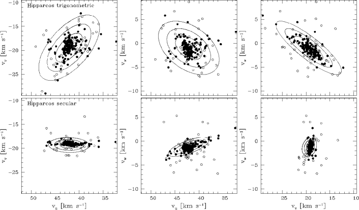
Figure 6: Top row: three-dimensional velocity distribution in Galactic Cartesian coordinates $(v_{u},v_{v},v_{w})$, based on Hipparcos trigonometric parallaxes, for the 197 P98 members with known radial velocities (cf. figure 16 in P98; symbol coding as in bottom row). The contours are centered on the (arithmetic) mean motion of all stars $(-42.07,-19.45,-0.96)$ km s^-1 (cf. table 3 in P98); they show the 1, 2, and 3$\sigma$ (i.e., 68.3, 95.4, and 99.73 per cent) confidence limits of the mean covariance matrix associated with the mean space motion (§6.4.2). All ‘outliers’ have space motions (based on Hipparcos proper motions and trigonometric parallaxes) which are consistent with the mean motion of the cluster. Bottom row: as top row, but using Hipparcos secular parallaxes (mean motion $(-42.15,-19.31,-1.21)$ km s^-1). Open symbols denote suspect secular parallaxes ($g_{\rm Hip}>9$; 50 stars).

The method described in §§2.2–2.3 assumes that the expectation values ${\rm E}({\mathbf{v}}_{i})$ of the individual stellar velocities ${\mathbf{v}}_{i}$ ($i=1,\ldots,n$) equal the cluster space motion ${\mathbf{v}}$ (cf. §3). A random internal velocity dispersion in addition to this common space motion is allowed and accounted for in the procedure, as random motions do not affect ${\rm E}({\mathbf{v}}_{i})$ by definition. However, a systematic velocity pattern, such as expansion or contraction, rotation, and shear, has not been taken into account in the modelling. The application of the procedure to data subject to velocity patterns is thus bound to lead to incorrect and/or biased results.

6.4.1 Pre-Hipparcos results

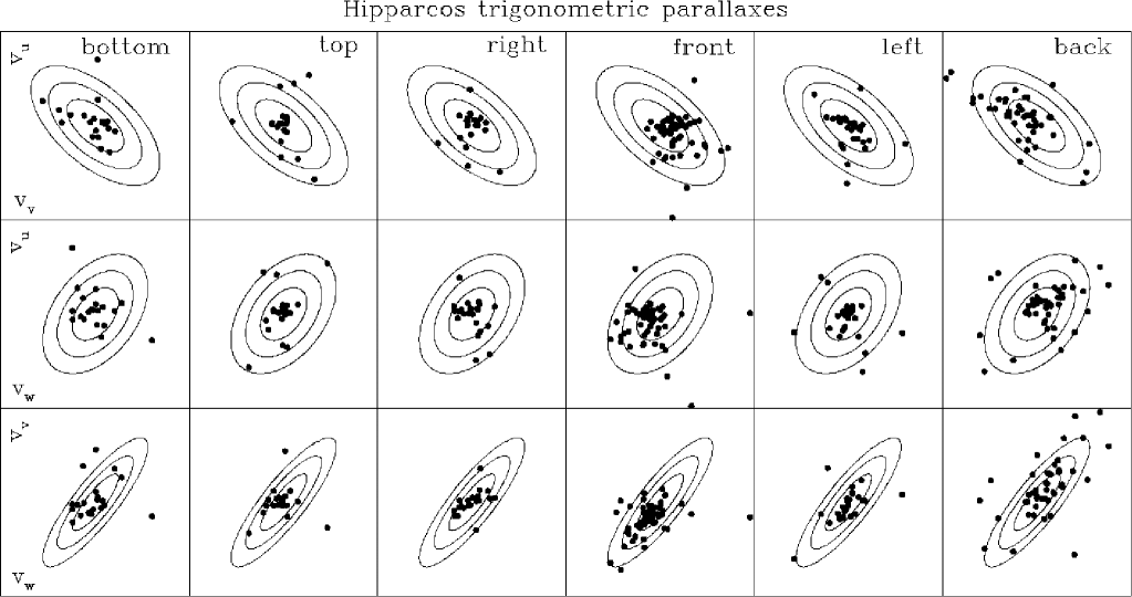
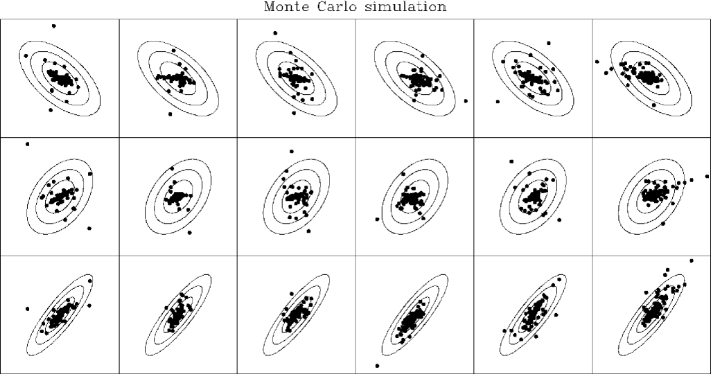
Figure 7: Top three rows: Hipparcos trigonometric parallax-based velocity field decomposition, with respect to the mean velocity $(v_{u},v_{v},v_{w})=(-42.07,-19.45,-0.96)$ km s^-1 in $20$ km s${}^{-1}\times 20$ km s${}^{-1}\times 20$ km s^-1 boxes, for the 197 P98 members with known radial velocities according to the location of the stars within the cluster (from the left column right: ‘bottom’ (21 stars), ‘top’ (21 stars), ‘right’ (22 stars), ‘front’ (59 stars), ‘left’ (28 stars), and ‘back’ (46 stars; §6.3) and from the top down: $v_{u}$ versus $v_{v}$, $v_{u}$ versus $v_{w}$, and $v_{v}$ versus $v_{w}$; velocity components in a Galactic Cartesian coordinate frame). The ellipses denote 1, 2, and 3$\sigma$ confidence regions of the mean motion and associated covariance matrix (§6.4.2). The bottom series of panels are similar to the top series, but show 500 Monte Carlo stars which share a common space motion exclusively (§6.4.3).

Many studies have been devoted to the detection or exclusion of velocity structure in the Hyades (see P98 for an overview), although $N$-body simulations of open clusters generally predict that, for gravitationally bound groups like the Hyades, velocity patterns are generally too small to be measured with present-day data (e.g., Dravins et al. 1997; §7.2 in P98). In view of the Hyades age ($\tau=625\pm 50$ Myr; P98), shear is not likely to be present in the core and corona: using $\sigma_{v}=0.30$ km s^-1 and a half-mass radius of 5 pc (Pels et al. 1975), it follows that $\tau\sim 20$ crossing times, which means that the central parts of the cluster are relaxed (cf. Hanson 1975). The Hyades age also puts a rough upper limit on the linear expansion coefficient $K\la 0.0016\leavevmode\nobreak\ {\rm km}\leavevmode\nobreak\ {\rm s}^{-1}\leavevmode\nobreak\ {\rm pc}^{-1}$ (resulting in a bias in the radial component of the maximum likelihood cluster space motion of $\la$$-0.07$ km s^-1). A global rotation of the cluster could be present, although Wayman (1967; cf. Wayman et al. 1965 and Hanson 1975) claimed that the cluster rotation about three mutually perpendicular axes is consistent with zero to within 0.05 km s^-1 pc^-1; Gunn et al. (1988) present (weak) evidence for rotation at the level of $\la$1 km s^-1 radian^-1 (cf. O’Connor 1914).

6.4.2 Hipparcos parallaxes: Perryman et al. (1998)

Figure 8(b) in P98 displays the three-dimensional velocity distribution $(v_{u},v_{v},v_{w})$ of the 197 P98 members with known radial velocities. Although the velocity residuals seem to show evidence for shear and/or rotation, notably for stars in the outer regions (figure 9 in P98), the systematic pattern can be explained by a combination of the transformation of the observables $(\pi_{\rm Hip},\mu_{\alpha^{\ast}},\mu_{\delta},v_{\rm rad,obs})$ to the linear velocity components $(v_{u},v_{v},v_{w})$ and the presence of Hipparcos data covariances: P98 show that the assumption of a common space motion for all members with a one-dimensional internal velocity dispersion of $0.30$ km s^-1, which allows averaging of the individual motions and associated covariance matrices for all stars, translates into a mean motion and associated mean covariance matrix (i.e., 1, 2, and 3$\sigma$ confidence regions) which adequately follow the observed velocity residuals (§7.2 and figures 16–17 in P98; cf. top row of Figure 6). Therefore, P98 conclude that the observed kinematic data of the Hyades cluster is consistent with a common space motion plus a 0.30 km s^-1 velocity dispersion, without the need to invoke the presence of rotation, expansion, or shear.

The motions of members beyond the tidal radius ($\sim$10 pc), as opposed to the motions of gravitationally bound members in the central parts of the cluster, are predominantly influenced by the Galactic tidal field (e.g., Pels et al. 1975). These (evaporated) stars do therefore not necessarily adhere to the strict pattern of a common space motion which is present in the core and corona. The systematic velocity distortions are hard to predict, analytically and numerically, as they depend critically on the details of the evaporation mechanism(s) (e.g., Terlevich 1987). They are hard to observe as well due to both the sparse sampling of ‘members’ and the uncertain criteria for membership in the outer regions of the cluster.

6.4.3 Hipparcos parallaxes: this study

Figure 7 (top series of panels) shows the Hyades velocity field, based on Hipparcos trigonometric parallaxes, for different spatial regions of the cluster (§6.3). The observed velocities are not identically distributed in each region but show systematic effects, although these are restricted to ‘the 3$\sigma$ confidence regions’. Notably the ‘front’ and ‘back’ of the cluster show differences, indicative of a coupling between position and velocity, i.e., a velocity pattern. Explanations for this trend include (1) a rotation of the cluster, (2) a shearing pattern with respect to an axis, and (3) a correlation between the trigonometric parallaxes $\pi_{\rm Hip}$ and their associated errors $\sigma_{\pi,{\rm Hip}}$ (cf. §7.2 in P98).

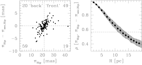
Figure 8: Left: an estimate of the Hipparcos trigonometric parallax error $\sigma_{\pi,{\rm Hip}}$ ($\pi_{\rm Hip}-\pi_{\rm sec,Hip}\approx\pi_{\rm Hip}-\pi_{\rm true}\equiv\Delta_{\pi,{\rm Hip}}$) versus the Hipparcos trigonometric parallax $\pi_{\rm Hip}$ for the 147 P98 Hyades members with non-suspect secular parallaxes ($g_{\rm Hip}\leq 9$). Every sample of stars with (nearly) equal true parallaxes shows a correlation between $\Delta_{\pi,{\rm Hip}}$ (or: $\sigma_{\pi,{\rm Hip}}$) and $\pi_{\rm Hip}$; we find a correlation coefficient $\rho=+0.56$. The dashed vertical line denotes the mean distance of the cluster ($D=46.34$ pc; $\pi=21.58$ mas; table 3 in P98). The numbers in the corners of the four quadrants denote the numbers of stars in the corresponding regions. Right: the mean correlation coefficient for 100 Monte Carlo realizations of a Hyades-like cluster as function of the cluster radius $R$. Each cluster has a homogeneous number density. The dots and vertical lines denote the mean value of $\rho$ and the corresponding standard deviation; the gray band denotes the $\pm 1\sigma$ region. The dashed horizontal line indicates the observed value $\rho=+0.56$.

(1) Rotation:

Given the observed velocity field, we determine the Galactic coordinates of the best-fitting rotation axis ($\ell_{\rm rot}$ and $b_{\rm rot}$) and the corresponding rotation period ($P_{\rm rot}$) by minimizing the dispersion of the velocity residuals with respect to the rotation axis, after adding a rotation pattern to the mean space motion. This results in the estimates $\ell_{\rm rot}\sim 131\aas@@fstack{\circ}5$, $b_{\rm rot}\sim+60\aas@@fstack{\circ}0$, and $P_{\rm rot}=68.0$ Myr (i.e., $\sim$0.10 km s^-1 pc^-1).

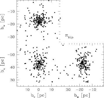
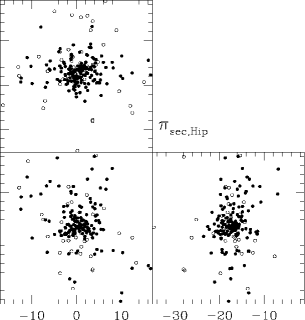
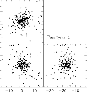
Figure 9: Left: three-dimensional distribution, based on Hipparcos trigonometric parallaxes, of the 218 P98 members in Galactic Cartesian coordinates $(b_{u},b_{v},b_{w})$ (in pc; cf. figures 8a–9 in P98). Some stars fall outside the plotted range. Middle: as left, but using Hipparcos secular parallaxes (154 stars with $g_{\rm Hip}\leq 9$ [filled symbols] and 64 stars with $g_{\rm Hip}>9$ [open symbols]). Right: as middle, but using Tycho–2 secular parallaxes (176/32 filled/open symbols).

(2) Shear:

A shear pattern with respect to an axis pointing towards $\ell_{\rm shear}$ and $b_{\rm shear}$ is described by a constant $P_{\rm shear}$ which expresses the strength of the shear. A least-squares fit returns $\ell_{\rm shear}\sim 131\aas@@fstack{\circ}5$, $b_{\rm shear}\sim+60\aas@@fstack{\circ}0$, and $P_{\rm shear}\sim 0.13$ km s^-1 pc^-1 (as our proper motion, parallax, and radial velocity data do not have enough discriminating power to reveal the subtle differences between a rotation and shear pattern, our fit returns a shear axis which is identical to the rotation axis listed above).

(3) Correlated trigonometric parallaxes and errors:

The lower series of panels in Figure 7 show a velocity field decomposition for a realistic Monte Carlo realization of the Hyades (500 stars, 10 pc radius, including Hipparcos data covariances) in which the stars share a common space motion exclusively. Despite the absence of intrinsic velocity structure, the ‘front’ and ‘back’ distributions do show a systematic pattern which resembles the observed distribution (upper series of panels) remarkably well. P98 (their §7.2) did already argue that correlated velocity residuals are a natural result of the presence of a correlation between the Hipparcos parallaxes $\pi_{\rm Hip}$ and the corresponding observational errors $\sigma_{\pi,{\rm Hip}}$ in a sample of Hyades members (left panel of Figure 8; we find a correlation coefficient $\rho=+0.56$ between $\pi_{\rm Hip}-\pi_{\rm sec,Hip}\approx\pi_{\rm Hip}-\pi_{\rm true}\equiv\Delta_{\pi,{\rm Hip}}$ and $\pi_{\rm Hip}$). Although the individual Hipparcos trigonometric parallaxes are not correlated with their associated observational errors, the selection of a set of stars with (nearly) equal true parallaxes, such as the members of an open cluster, induces the presence of a correlation in the sample: Hyades with large observed parallaxes are, in general, more likely to have $\Delta_{\pi,{\rm Hip}}\equiv\pi_{\rm Hip}-\pi_{\rm true}>0$ than $\sigma_{\pi,{\rm Hip}}<0$ (and vice versa for Hyades with small observed parallaxes). The strength of this correlation between the (sign of the) parallax error and the observed parallax depends on the intrinsic size of the cluster: a small cluster gives a small spread in true parallaxes, which implies a large correlation. The right panel of Figure 8 shows the mean correlation coefficient derived from Monte Carlo realizations of a Hyades-like cluster as function of the cluster radius $R$. The observed correlation coefficient $\rho=+0.56$ implies $R\sim 10$–$15\leavevmode\nobreak\ {\rm pc}\sim 1.0$–$1.5\leavevmode\nobreak\ r_{\rm t}$, which is a very reasonable definition for the size of the Hyades cluster.

Discussion:

The analysis presented above shows that the systematic velocity pattern displayed in Figure 7 can be due to rotation, shear, and/or a correlation between $\pi_{\rm Hip}$ and $\sigma_{\pi,{\rm Hip}}$. Both rotation and shear provide an equally good representation of the observations, but imply a significant systematic velocity of $\sim$1 km s^-1 at the tidal radius of the cluster ($r_{\rm t}\sim 10$ pc). Unmodelled systematic velocities at the level of 1–2 km s^-1 in the outer regions of the cluster ($r_{\rm t}\la r\la 2r_{\rm t}$) would lead to systematic secular parallax errors as large as 0.9–1.8 mas. These values, however, are a factor 3–6 larger than the observed upper limit of 0.3 mas at $r\sim 20$ pc (Figure 5; §6.3), which argues against an explanation of the velocity pattern in terms of rotation or shear. There is, moreover, also a direct argument in favour of the apparent velocity pattern not being caused by rotation or shear, but by the correlation between the observed parallaxes and the parallax errors instead, for this should result in an apparent rotation or shear axis pointing towards $(b_{u},b_{v},b_{w})\times(v_{u},v_{v},v_{w})$, i.e., $(\ell,b)=(116^{\circ}\!,+48^{\circ}\!)$ ($[b_{u},b_{v},b_{w}]$ and $[v_{u},v_{v},v_{w}]$ denote, respectively, the position and velocity vector of the cluster center expressed in Galactic Cartesian coordinates). This axis coincides within $15^{\circ}\!$ with the rotation and shear axes found above. We therefore conclude that the observed correlation between the Hipparcos trigonometric parallaxes and their associated random errors (Figure 8) is mainly responsible for the (apparent) velocity structure of the Hyades (Figure 7; cf. P98).

6.4.4 Secular parallaxes

Studying the Hyades velocity field using secular parallaxes, which were derived under the assumption of a specific velocity field, is of limited scientific merit. We therefore restrict such an analysis to the straightforward comparison of the input and output velocity fields (bottom row of Figure 6), which turn out to be fully consistent. A systematic pattern as observed in the trigonometric parallax velocity field (§6.4.3) is absent in the secular parallax velocity field (not shown).

6.5 Summary

Monte Carlo tests combined with the uncertainty of the tangential component of the cluster space motion set the maximum expected systematic Hipparcos secular parallax error at $\sim$0.30 mas (§6.1). This value is consistent with the facts that (1) the secular parallaxes as a set are statistically consistent with the Hipparcos trigonometric parallaxes within $\la$0.10 mas (Figure 3; §5), and (2) secular parallaxes for stars in the inner and outer regions of the Hyades do not differ significantly, i.e., at the $\sim$0.30 mas level or larger (Figure 5; §6.3). We conclude that secular parallaxes for Hyades within at least $r\la 2r_{\rm t}\sim 20$ pc of the cluster center can be regarded as absolute, i.e., having systematic errors smaller than $\sim$0.30 mas.

The Hipparcos trigonometric parallax errors are correlated on angular scales of a few degrees with ‘amplitudes’ smaller than $\sim$$0.75$–$1.00$ mas per star (§6.2). The mean trigonometric parallax of the Hyades, however, is accurate to within $\la$0.10 mas, as regions with positive and negative contributions cancel when averaging parallaxes over the large angular extent of the cluster.

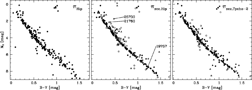
Figure 10: Colour-absolute magnitude diagrams of the Hyades based on Hipparcos trigonometric parallaxes (left; 218 P98 members) and Hipparcos secular (middle; 218 P98 members plus 15 new candidates) and Tycho–2 secular parallaxes (right; 208 P98 members plus 23 photometric BDA members; $V$ magnitude (field H5) and $(B-V)$ colour (field H37) from the Hipparcos Catalogue). Most P98 stars below the main sequence in the left panel are ‘possible members’ (i.e., column (x) is ‘?’ in their table 2; cf. figure 21 in P98). Filled symbols in the right panels have $g_{\rm Hip/Tycho-2}\leq 9$ while open symbols have $g_{\rm Hip/Tycho-2}>9$. The 15 triangular symbols in the middle panel are the new Hipparcos candidates (§5.2); the three stars with $g_{\rm Hip}\leq 9$ are labeled with their Hipparcos number. The giant region contains three(!) filled and two open symbols. The triangular symbols in the right panel represent 23 photometric BDA members (§5.3; filled triangles for $g_{\rm Tycho-2}\leq 9$ and open triangles for $g_{\rm Tycho-2}>9$). The giant region contains four(!) filled and one open symbol. Some faint stars ($V\mathrel{{\hbox to0.0pt{\lower 3.0pt\hbox{$\sim$}\hss}}\raise 2.0pt\hbox{$>$}}8.5$ mag, $M_{V}\mathrel{{\hbox to0.0pt{\lower 3.0pt\hbox{$\sim$}\hss}}\raise 2.0pt\hbox{$>$}}5.2$ mag) in the right panel have significant $(B-V)$ errors, up to several tenths of a magnitude (§8).

The observed lack of significant systematics in the secular parallaxes puts an upper limit on the size of possible velocity patterns (rotation or shear) of a few hundredths of a km s^-1 pc^-1 (§6.4.3). This upper limit, in its turn, strongly suggests that the observed systematics in the trigonometric parallax-based velocity field (Figure 7) are due to the presence of a correlation between the Hipparcos parallaxes and their associated random errors in our sample of Hyades.

7 Spatial structure

At the mean distance of the Hyades, a parallax uncertainty of $\sigma_{\pi}$ (mas) corresponds to a distance error of $\sigma_{\pi}D^{2}/1000\sim 2\sigma_{\pi}$ pc ($D\sim 45$ pc). Typical Hipparcos parallax errors are 1.0–1.5 mas, thus yielding a $\sim$2–3 pc distance resolution. Typical Hipparcos secular parallaxes are $\sim$3 times more accurate than the trigonometric values (§5.4). However, because the Hipparcos resolution is already sufficient to resolve the internal structure of the Hyades (with core and tidal radii of 2.7 and 10 pc, respectively; §4.1), secular parallaxes cannot fundamentally improve upon the P98 results regarding, e.g., the three-dimensional spatial distribution of stars in the cluster, including the shape of the core and corona and flattening of the halo, ‘the Hyades distance’, the density and mass distribution of stars in the cluster, its gravitational potential, moments of inertia, etc. (§§7–8 in P98; we investigated all aforementioned examples using secular parallaxes, but were unable to obtain results which had not already been derived by P98). Figure 9, for example, shows the three-dimensional distribution of the 218 P98 members. Although the internal spatial structure of the Hyades is resolved by the Hipparcos trigonometric parallaxes, the Hipparcos secular parallaxes do provide a sharper view.

8 Colour-absolute magnitude diagram

The colour-absolute magnitude and HR diagrams of the Hyades cluster have been studied extensively, mainly owing to the small distance of the cluster. Among the advantages of this proximity are the negligible interstellar reddening and extinction (e.g., Crawford 1975; Taylor 1980; $E(B-V)=0.003\pm 0.002$ mag) and the possibility to probe the cluster (main sequence) down to low masses relatively easily. As mentioned in §1, the significant cluster depth along the line of sight has always complicated pre-Hipparcos stellar evolutionary modelling (cf. §9.0 in P98). Unfortunately, even Hipparcos parallax uncertainties (typically 1.0–1.5 mas) translate into absolute magnitude errors of $\ga$0.10 mag at the mean distance of the cluster ($D\sim 45$ pc), whereas $V$-band photometric errors only account for $\la$0.01 mag uncertainties for most members. The Hipparcos secular parallaxes derived in §5 are on average a factor $\sim$3 times more precise than the Hipparcos trigonometric values (i.e., $\sigma_{\pi,{\rm sec,Hip}}\la 0.5\leavevmode\nobreak\ {\rm mas}\sim 0.05\leavevmode\nobreak\ {\rm mag}$; §5.4). The maximum expected systematic error in the secular parallaxes is $\la$$0.3\leavevmode\nobreak\ {\rm mas}$ or $\la$$0.03\leavevmode\nobreak\ {\rm mag}$ (§6.5). Secular parallaxes therefore allow the construction of a well-defined and well-calibrated Hyades colour-absolute magnitude (and HR) diagram.

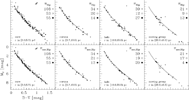
Figure 11: Colour-absolute magnitude diagrams of the Hyades (218 P98 members) based on Hipparcos trigonometric (top row) and Hipparcos secular (bottom row) parallaxes for four different spatial regions within the cluster: the core ($r<5.7$ pc; first column), the corona ($5.7\leq r<10$ pc; second column), the halo ($10\leq r<20$ pc; third column), and the moving group population ($20\leq r<40$ pc; fourth column). In each panel, the division of stars according to their three-dimensional distance $r$ to the cluster center $(b_{u},b_{v},b_{w})=(-43.37,0.40,-17.46)$ pc (in Galactic Cartesian coordinates) is based on the Hipparcos secular parallax. The gray lines outline Schwan’s (1991; his table 3) Hyades main sequence; this calibration is not necessarily the optimal one but is only shown for reference. The numbers preceding the open asterisks denote the total number of stars in each panel. Open symbols denote stars which might have ‘peculiar’ HR diagram positions: (1) kinematically deviant stars, i.e., $g_{\rm Hip}>9$; (2) (close) multiple stars, i.e., either column (s) in P98’s table 2 is ‘SB or RV’ or column (u) is one of ‘C G O V X S’; (3) photometrically variable stars, i.e., Hipparcos field H52 is one of ‘D M P R U’; (4) stars with inaccurate Hipparcos $(B-V)$ photometry, i.e., $\sigma_{(B-V)}>0.05$ mag; or (5) suspect objects (HIP 20901, 21670, 20614; §9.2 in P98). Filled symbols thus denote kinematically high-fidelity photometrically non-variable single members with reliable photometry.

Figure 10 shows colour-absolute magnitude diagrams of the Hyades based on Hipparcos trigonometric (left), Hipparcos secular (middle), and Tycho–2 secular parallaxes (right). The Hipparcos secular parallax diagram shows a narrow main sequence consisting of kinematic members ($g_{\rm Hip}\leq 9$; filled symbols; cf. Figure 13). Kinematically deviant stars ($g_{\rm Hip}>9$; open symbols) are likely either non-members and/or close multiple stars (§4.3). Most of the 15 new Hipparcos candidates (open triangular symbols; §4.2) do not follow the main sequence. This is not surprising, as secular parallaxes for most of these stars are inconsistent with their trigonometric parallaxes, suggestive of non-membership. The three candidates with $g_{\rm Hip}\leq 9$ (filled triangles) identified in §5.2 are labeled. Only HIP 19757 lies close to the main sequence and is a likely new member (cf. Table 7).

The right panel of Figure 10 shows, besides a narrow cluster main sequence consisting of kinematic members ($g_{\rm Tycho-2}\leq 9$; filled circles), a well-defined binary sequence for $0.45\mathrel{{\hbox to0.0pt{\lower 3.0pt\hbox{$\sim$}\hss}}\raise 2.0pt\hbox{$>$}}(B-V)\mathrel{{\hbox to0.0pt{\lower 3.0pt\hbox{$\sim$}\hss}}\raise 2.0pt\hbox{$>$}}0.70$ mag. Most of the photometrically deviant stars are low-probability kinematic members ($g_{\rm Tycho-2}>9$; open circles), most likely indicating non-membership. The 23 photometric BDA members (§5.3) are indicated by triangles (filled for $g_{\rm Tycho-2}\leq 9$; open for $g_{\rm Tycho-2}>9$). About half of them do not follow the main sequence. Most of these objects, nonetheless, seem secure kinematic members ($g_{\rm Tycho-2}\leq 9$; cf. §5.3). These stars are possibly interlopers but most likely they are members with inaccurate $(B-V)$ photometry: objects lacking accurate ground-based photometric observations, most likely as a result of being pre-Hipparcos non-members, generally have Hipparcos $(B-V)$ values derived from Tycho photometry (Hipparcos field H39 = ‘T’). Corresponding $(B-V)$ errors can reach several tenths of a magnitude for stars fainter than $V\sim 8.5$ mag ($M_{V}\sim 5.2$ mag). Hipparcos $(B-V)$ values for faint pre-Hipparcos members contained in the Hipparcos Catalogue, on the other hand, are often carefully selected accurate ground-based measurements (field H39 = ‘G’); this explains the presence of a well-defined main sequence down to faint magnitudes ($V\sim 11$–$12$ mag).

Figure 11 compares colour-absolute magnitude diagrams for different regions within the cluster (core, corona, halo, and moving group; §4.1). Secular parallaxes clearly improve the definition of the main sequence as compared to Hipparcos trigonometric parallaxes in the central parts of the cluster. They also significantly narrow the main sequence for stars in the halo ($10\leq r<20$ pc). The relatively large spread in the Hipparcos secular parallax panel for $20\leq r<40$ pc is probably due to uncertain membership assignment (cf. §6.4.2), combined with inaccurate photometry, stellar multiplicity, and/or suspect secular parallaxes. The latter uncertainty is possibly related to unmodelled low-amplitude velocity patterns in the very outer parts of the cluster ($r\ga 2r_{\rm t}$; but see §§6.4–6.5).

9 Constructing the Hertzsprung–Russell diagram

The secular parallaxes derived in §5 constrain the locations of stars in the colour-absolute magnitude diagram with unprecedented precision (§8). An interpretation of these high-quality observations in terms of stellar evolutionary models with appropriately chosen input physics (§9.1) can provide a wealth of information on the fundamental properties of the Hyades cluster itself, such as its age and metallicity (§9.2), as well as on the characteristics of stars and stellar evolution in general (§§9.3–9.4).

9.1 Theoretical stellar evolutionary models

Stellar evolutionary models have been highly successful in explaining the structure and evolution of stars (e.g., Cox & Giuli 1968; Kippenhahn & Weigert 1990). Numerical stellar evolutionary codes suffer from daunting practical problems, owing to, e.g., the large dynamical range for the various quantities of interest such as temperature, pressure, and density (e.g., Schwarzschild 1958; Henyey et al. 1959). Moreover, they suffer from major uncertainties in the appropriate input physics (e.g., Lebreton et al. 1995, 2000; Kurucz 2000). The most important of these uncertainties are, for Hyades main sequence stars, related to: (1) stellar atmosphere models, including issues related to atomic and molecular opacities and internal structure–external boundary conditions (§10.1); and (2) the treatment of turbulent convection, including issues related to convective core and envelope overshoot. Besides these two major uncertainties, numerous other physical phenomena are generally either not or only partially taken into account: (transport processes due to) stellar rotation (§10.3), variability and/or pulsational instability (§10.3), chromospheric activity (§10.1), mass loss (§10.4), binary evolution, the evolution towards the zero-age main sequence, etc. Moreover, stellar evolutionary models are generally calibrated by using the Sun as benchmark. Although the phenomenological treatment of convection in models is considered appropriate for Sun-like stars, this is not necessarily the case for stars with other mass, metallicity, and/or stellar evolutionary status. Related to the latter issue is the important open question to what extent the characteristics of convection vary with location in a convection zone. A detailed study of the secular parallax-based locations of Hyades in the colour-absolute magnitude and HR diagrams of the cluster has the potential to shed light on some of the abovementioned issues (e.g., Lebreton 2000).

9.2 Helium content, metallicity, and age of the Hyades

CESAM:

P98 used the CESAM evolutionary code (Morel 1997) to interpret the Hipparcos HR diagram of the Hyades (their §9). In order to derive the cluster Hydrogen, Helium, and metal abundances by mass ($X\equiv 1-Y-Z$, $Y$, and $Z$, respectively), P98 fitted model zero-age main sequences to the observed trigonometric parallax-based zero-age main sequence positions of 19 single low-mass members. By treating $Y$ and $Z$ as free parameters with the boundary condition that the inferred metal content of the Hyades be consistent with the mean spectroscopically determined metallicity $[{\rm Fe/H}]=+0.14\pm 0.05$, P98 found $(X,Y,Z)=(0.716,0.260\pm 0.020,0.024\pm 0.003)$. The P98 $[{\rm Fe/H}]$ value is a well-established quantity (cf. $[{\rm Fe/H}]\ga+0.12\pm 0.03$ Cayrel et al. 1985; $+0.13\pm 0.02$ Boesgaard 1989 and Boesgaard & Friel 1990). Unfortunately, the uncertainty on the derived Helium content of the cluster, combined with the existing uncertainty on the Helium content of the Sun (e.g., Brun et al. 1998), still prevents a definitive answer to the question whether the Helium content of the Hyades is sub-Solar or not (e.g., Strömgren et al. 1982; Hardorp 1982; Dobson 1990; Swenson et al. 1994; Pinsonneault et al. 1998).

After establishing the chemical composition of the Hyades, P98 derived a nuclear age $\tau=625\pm 50$–$100$ Myr by fitting CESAM isochrones to the upper main sequence of the trigonometric parallax-based colour-absolute magnitude diagram (their figures 21–23 and §9.2; cf. $\tau=600\pm 50$ Myr from Torres et al. 1997a, c).

Padova:

For an interpretation of the HR diagram of the Hyades, the latest Padova isochrones (Girardi et al. 2000a) offer the advantage that they include (post) red giant branch evolution.

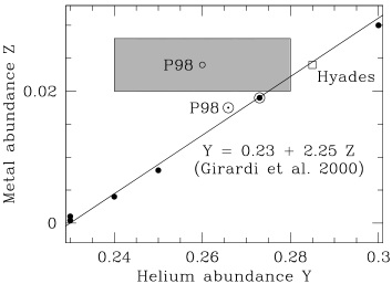
Figure 12: The six $(Y,Z)$ values (solid dots) for which Girardi et al. (2000a) present isochrones; the solid line shows the underlying relation $Y=Y_{\rm p}+(\Delta Y/\Delta Z)\cdot Z=0.23+2.25\cdot Z$ (§9.2). The $\odot$ symbol, which coincides with a solid dot, denotes the position of the Sun $(Y,Z)_{\odot}=(0.273,0.019)$. The open dot and corresponding gray box labeled ‘P98’ denote the P98 Hyades value and corresponding 1$\sigma$ uncertainty; the $\odot$ symbol labeled ‘P98’ denotes P98’s Solar value $(Y,Z)_{\odot}=(0.2659,0.0175)$. The open square at $(Y,Z)=(0.285,0.024)$ labeled ‘Hyades’ is discussed in §9.2.

The six $(Y,Z)$ pairs discussed by Girardi et al. were not randomly chosen but follow a fixed $Y(Z)$ relation (Figure 12), which is inspired by the understanding of the origin of Helium and metals in the universe: $Y\sim Y_{\rm p}+(\Delta Y/\Delta Z)\cdot Z$, where $Y_{\rm p}=0.23$ is the primordial Helium abundance, and $\Delta Y/\Delta Z=2.25$ is the stellar evolution Helium-to-metal enrichment ratio (e.g., Faulkner 1967; Pagel & Portinari 1998; Lebreton et al. 1999). The $Y(Z)$ relation implies we cannot obtain Padova isochrones which are consistent with both the Helium content and metallicity of the Hyades as derived by P98. Taking the latter fixed at $Z=0.024$, and interpolating between the sets $(Y,Z)=(0.273,0.019)$ and $(0.300,0.030)$, provides isochrones with $Y=0.285$ (open square in Figure 12). Although this value is inconsistent at the 1.25$\sigma$ level with P98’s value, it cannot be considered inappropriate for the Hyades (VandenBerg & Bridges 1984).

As the interpolation between published isochrones is practically impossible after crossing the Hertzsprung gap, we use Girardi’s Solar-metallicity $(Y,Z,\tau\leavevmode\nobreak\ [{\rm Myr}])=(0.273,0.019,631)$ isochrone for a comparison with the Hyades giants (§10.4).

9.3 A high-fidelity stellar sample

Figure 13: Colour-absolute magnitude diagram for 92 high-fidelity members (§9.3). This sample excludes all members beyond 40 pc from the cluster center, multiple stars, and stars with suspect secular parallaxes. The absolute magnitudes have been computed using the observed $V$-band magnitudes (Hipparcos field H5) and secular parallaxes (§5; Table LABEL:tab:data_1). The $(B-V)$ colours were directly taken from the Hipparcos Catalogue (field H37). The gaps between $(B-V)=0.15$ and $0.20$, between $(B-V)=0.30$ and $0.35$, and the gap around $(B-V)=0.95$ mag are caused by the suppression of double, multiple, and peculiar stars from our sample (cf. figure 21 in P98); the region between $(B-V)=0.30$ and $(B-V)=0.35$ mag, e.g., is occupied by Am-type stars, which have a high incidence of duplicity (§10.2). The lines point at two conspicuous features in the main sequence, the so-called Böhm–Vitense gaps (§10.2). The ‘gaps’ and corresponding ‘turn-offs’ are most likely caused by sudden changes in the properties of convective atmospheres (cf. de Bruijne et al. 2000). Figure 18(a) presents the corresponding theoretical HR diagram ($\log L$ versus $\log T_{\rm eff}$) for the same sample of stars.

Following P98, we restrict attention to a high-fidelity subset of members for the study of the HR diagram. We do not consider suspect kinematic members and stars which have deviant HR diagram positions for known reasons. We exclude the 16 stars beyond 40 pc from the cluster center and all (possible) close multiple systems (98 spectroscopic binaries, Hipparcos DMSA–‘G O V X S’ stars, and stars with $g_{\rm Hip}>9$). We furthermore reject 11 stars which are variable (Hipparcos field H52 is one of ‘D M P R U’) or have large photometric errors ($\sigma_{(B-V)}>0.05$ mag), as well as the suspect objects HIP 20901, 21670, and 20614 (§9.2 in P98; cf. Wielen et al. 2000).

The final sample contains 90 single members. These stars follow the main sequence (cluster isochrone) from $(B-V)\sim 1.43$ mag (late-K/early-M dwarfs; $M\ga 0.5\leavevmode\nobreak\ M_{\odot}$) to $(B-V)\sim 0.10$ mag (A7IV stars; $M\sim 2.4\leavevmode\nobreak\ M_{\odot}$). Two of the stars are evolved red giants ($\epsilon$ and $\gamma$ Tau; §10.4 and B.1). The two components of the ‘resolved spectroscopic binary’ $\theta^{2}$ Tau, located in the turn-off region of the cluster (§10.3 and B.3; cf. P98), contribute significant resolving power for distinguishing between different evolutionary models as well as between different isochrones from one evolutionary code. We therefore add them as single stars to our sample, bringing the total number of objects to 92.

Figure 13 shows, for these 92 stars, the colour versus secular parallax-based absolute magnitude diagram (cf. Figures 10–11). It shows, besides a well-defined and very narrow main sequence, turn-off region, and giant clump, substructure in the form of two ‘gaps’/‘turn-offs’ in the main sequence around $(B-V)\sim 0.30$ and $\sim$$0.45$ mag (cf. de Bruijne et al. 2000). These features are also present in the Tycho–2 secular parallax-based diagram (right panel of Figure 10), but are not clearly discernible in the lower quality trigonometric parallax-based version (left panel of Figure 10). In §10.2, we will identify these ‘turn-offs’ with so-called Böhm–Vitense gaps, which are most likely related to convective atmospheres. Although the reality of the turn-offs in the ‘cleaned’ secular parallax colour-magnitude diagram is hard to establish beyond all doubt, the simultaneous existence of both a turn-off and an associated gap at a location which coincides with predictions made by stellar structure models (see §10.2) strongly argues in favour of them being real (cf. Kjeldsen & Frandsen 1991, and references therein).

9.4 $(B-V)$–$M_{V}$ $\longrightarrow$ $\log T_{\rm eff}$–$\log(L/L_{\odot})$

In order to compare the locations of Hyades in the HR diagram to theoretical isochrones, we need to transform the observables $(B-V)$ and $M_{V}$ to the theoretical quantities $T_{\rm eff}$ and luminosity $L$. The usual procedure is to derive $T_{\rm eff}$ from $(B-V)$ and then to compute the bolometric correction in the $V$-passband, ${\rm BC}_{V}$, from $T_{\rm eff}$; $\log(L/L_{\odot})$ then follows from $M_{\rm bol}-M_{\rm bol,\odot}$, where $M_{\rm bol,\odot}=4.74$ mag (Bessell et al. 1998; cf. footnote 16; the IAU value for the solar bolometric magnitude is 4.75 mag). Both transformations depend on metallicity $[{\rm Fe/H}]$ and on surface gravity $\log g$, i.e., stellar evolutionary status.

9.4.1 Previous work

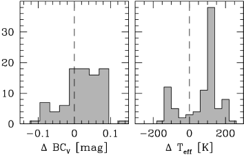
Figure 14: The difference between bolometric corrections (left) and effective temperatures (right) derived using calibration (1) (Bessell et al. (1998) plus an Alonso et al. (1996) metallicity correction to $[{\rm Fe/H}]=+0.14$) and calibration (2) (Lejeune et al. (1998) for $[{\rm Fe/H}]=+0.14$) for 92 high-fidelity members (§9.3), excluding the giants $\epsilon$ and $\gamma$ Tau; $\Delta$ is defined as calibration (1) minus (2). Most stars with $\Delta T_{\rm eff}<0$ K have $(B-V)\geq 1.0$ mag, indicating that calibrations (1) and (2) differ systematically with effective temperature itself.

Numerous empirical and theoretical calibrations have been proposed in the past, each of which has its own validity in terms of $\log g$, $T_{\rm eff}$, $(B-V)$, and/or $[{\rm Fe/H}]$ (e.g., Flower 1977, 1996; Buser & Kurucz 1992; Gratton et al. 1996). There is a large uncertainty in and systematic disagreement between the different $(B-V)$–$T_{\rm eff}$ relations. This is partly caused by the uncertain Solar photospheric abundances and ill-defined $(B-V)$ colour of the Sun (e.g., appendix C in Bessell et al. 1998), but also partly by the specific choice of the $(B-V)$ index. This colour is particularly sensitive to opacity problems, mainly related to metal lines and molecular electronic transitions in the UV-blue-optical, especially for cool stars ($T_{\rm eff}\la 4500$ K; e.g., Lejeune et al. 1998; Bessell et al. 1998). The effects of model uncertainties, related to opacities and the treatment of convection (§9.1), on theoretical calibrations are often non-negligible, especially for K/M giants and low-mass dwarfs (e.g., Blackwell et al. 1991; cf. table 4 in Houdashelt et al. 2000). The main reason for our ignorance is the lack of a representative set of stars with (model-)independently determined effective temperatures (e.g., Code et al. 1976; Ridgway et al. 1980; Blackwell & Lynas–Gray 1994). Differences between effective temperature scales, established by empirical or theoretical calibrations, are generally smaller than $\sim$200–400 K (Castelli 1999; Gardiner et al. 1999).

We consider two calibrations: (1) Bessell et al. (1998) in combination with Alonso et al. (1996; §9.4.2), roughly following P98; and (2) Lejeune et al. (1998; §9.4.3).

9.4.2 Calibration (1)

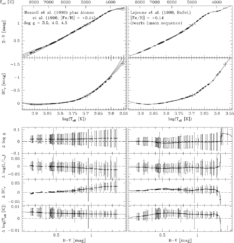
Figure 15: Theoretical quantities $\log T_{\rm eff}$, ${\rm BC}_{V}$, $\log(L/L_{\odot})$, and $\log g$ derived from $(B-V)$ and $M_{V}$ (the latter based on Hipparcos secular parallaxes) using Bessell et al. (1998) plus Alonso et al. (1996; left column) and Lejeune et al. (1998; right column; §§9.4.2–9.4.3). Left column: the gray curves in the top two panels show the Bessell et al. relation for $[{\rm Fe/H}]=0$ and $\log g=3.5,4.0$, and $4.5$ (from bottom to top along the vertical line $\log(T_{\rm eff}[{\rm K}])=3.9$, respectively); the (tiny) dots and crosses show the (metallicity corrected) values and uncertainties for the 92 high-fidelity Hyades (§9.3), excluding the giants $\epsilon$ and $\gamma$ Tau. The bottom four panels show the effect of correcting the Bessell et al. calibration for the non-Solar Hyades metallicity $[{\rm Fe/H}]=+0.14$ on (from the top panel down) $\log g$, $\log(L/L_{\odot})$, ${\rm BC}_{V}$, and $\log T_{\rm eff}$. The difference $\Delta x$ is defined as $\Delta x\equiv x_{[{\rm Fe/H}]=+0.14}-x_{[{\rm Fe/H}]=0}$ for $x=\log g$, etc. The faint M dwarf HIP 15720 ($(B-V)=1.431\pm 0.004$ mag) has no Bessell et al. solution for $[{\rm Fe/H}]=0$. The gray line in the bottom panel follows Alonso’s eq. (1). Right column: as left column, but using the Lejeune et al. relation for dwarfs with $[{\rm Fe/H}]=+0.14$. The bottom four panels show the effect of going from $[{\rm Fe/H}]=0$ to $[{\rm Fe/H}]=+0.14$ by means of interpolation. The apparent discontinuities of the gray lines in the lower panels are caused by the peculiar behaviour of the Lejeune et al. $[{\rm Fe/H}]=+0.50$ relation (their table 9) around $(B-V)=1.30$ mag. Several stars with $(B-V)>1.30$ mag fall outside the plotted ranges in the bottom panels.

Bessell et al. (1998) present broad-band colour, bolometric correction, and effective temperature calibrations for O to M stars, based on Kurucz’s (1995) ATLAS9 model atmospheres. Their tables 1 and 3 relate $T_{\rm eff}$, $\log g$, $(B-V)$, and ${\rm BC}_{V}$, based on Solar-metallicity models with convective core overshoot ($\alpha_{\rm MLT}=1.25$).

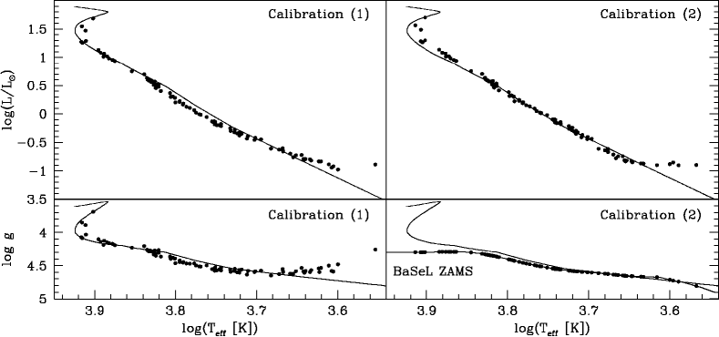
Figure 16: The $\log T_{\rm eff}$–$\log(L/L_{\odot})$ (top) and $\log T_{\rm eff}$–$\log g$ (bottom) diagrams for the same 92 stars as in Figure 18(a) and (b), excluding the giants $\gamma$ and $\epsilon$ Tau, but using calibration (1) (§9.4.2; left) and (2) (§9.4.3; right) for all stars. The curves denote the 625 Myr CESAM isochrones.

We use an iterative scheme to determine $\log T_{\rm eff}$, $\log(L/L_{\odot})$, and $\log g$ from the measured $(B-V)$ and $M_{V}$ values, in which we correct for the non-Solar metallicity of the Hyades according to Alonso et al. (1996; their eq. 1). Step 1 involves the determination of $\log T_{\rm eff}$ for $[{\rm Fe/H}]=0$, from a given $\log g$ and measured $(B-V)$. After differentially applying Alonso’s metallicity correction for $[{\rm Fe/H}]=+0.14$ in step 2, the corrected $\log T_{\rm eff}$ provides ${\rm BC}_{V}$, and thus $\log(L/L_{\odot})$. Step 3 involves the determination of $\log g=\log(4\pi GM\sigma_{\rm Boltzmann}T^{4}_{\rm eff}L^{-1})$ using stellar masses $M$ from P98 (§9.4.5). This recipe is repeated (typically 3 times) until convergence is achieved in the sense that $\log g$ remains constant; the final results do not depend on the initial estimate $\log(g[{\rm cm\leavevmode\nobreak\ s}^{-2}])=4.5$.

First-order error analysis allows an estimation of the uncertainties on the derived quantities. We assume that $\sigma_{\log(L/L_{\odot})}$ is influenced by both $\sigma_{M_{V}}$ and $\sigma_{{\rm BC}_{V}}$, which in their turn are influenced by $\sigma_{V}$ plus $\sigma_{\pi}$ and $\sigma_{\log T_{\rm eff}}$, respectively. We assume that $\sigma_{\log T_{\rm eff}}$ is influenced by both $\sigma_{(B-V)}=\min(\sigma_{(B-V),{\rm observed}},0.010\leavevmode\nobreak\ {\rm mag})$ and $\sigma_{M}=0.10\leavevmode\nobreak\ M_{\odot}$ (P98); we neglect the contribution of $\sigma_{\log g}$ to $\sigma_{\log T_{\rm eff}}$ as it is typically an order of magnitude smaller than the other contributors (cf. Castelli et al. 1997).

9.4.3 Calibration (2)

Lejeune et al. (1998) present (semi-)empirical calibrations linking $T_{\rm eff}$, $(B-V)$, $\log g$, and ${\rm BC}_{V}$ for $[{\rm Fe/H}]$ between $-3.5$ and $+1.0$ based on BaSeL spectral energy distributions (Basel Stellar Library version 2.0; their tables 1–10). In the range of stellar parameters considered here, these calibrations use Kurucz (1995) ATLAS9 model atmospheres. The presentation of the data, which is relevant for dwarfs ($\log g\ga 3.75$), allows a direct determination of $\log T_{\rm eff}$, $\log(L/L_{\odot})$, and $\log g$ from the measured $(B-V)$ and $M_{V}$ for $[{\rm Fe/H}]=+0.14$ by means of interpolation between table 1 ($[{\rm Fe/H}]=0$) and table 9 ($[{\rm Fe/H}]=+0.50$), without relying on stellar mass information. We derive $\sigma_{\log(L/L_{\odot})}$ and $\sigma_{\log T_{\rm eff}}$ as in §9.4.2.

9.4.4 Results for dwarfs

We applied calibrations (1) and (2) to the set of 92 members described in §9.3, excluding the giants $\epsilon$ and $\gamma$ Tau (Appendix B.1), using absolute magnitudes $M_{V}$ based on Hipparcos secular parallaxes (§5). Details for the spectroscopic binary $\theta^{2}$ Tau are given in Appendix B.3

For a given calibration, the bolometric corrections are relatively well defined, except at lower masses (i.e., redder $(B-V)$, lower $T_{\rm eff}$; Figures 14–15). Effective temperatures, on the other hand, are quite uncertain, especially at higher masses. Moreover, a comparison of the effective temperatures derived from calibrations (1) and (2) reveals significant systematic differences (at the level of $\sim$100 K; Figure 14) as a function of $T_{\rm eff}$ itself. Taking the non-Solar metallicity of the Hyades into account significantly changes the derived parameters, and notably the effective temperatures (Figure 15).

In order to establish which calibration is to be preferred, we compared the effective temperatures following from Bessell’s and Lejeune’s relations (for $[{\rm Fe/H}]=0$ as well as $[{\rm Fe/H}]=+0.14$) with a number of previously established effective temperature scales for the Hyades (Bessell et al. [1998; with and without overshoot; see footnote 15] plus Alonso et al. [1996; $[{\rm Fe/H}]=0$ and $+0.14$]; Lejeune et al. [1998; $[{\rm Fe/H}]=0$ and $+0.14$]; Allende Prieto & Lambert [1999; table 1]; Varenne & Monier [1999; table 2]; P98 [table 8]; and Balachandran [1995; table 4]). This analysis reveals effective temperature differences, which sometimes vary systematically with effective temperature itself (cf. Figure 14), up to $\sim$300 K. Unfortunately, none of these scales is truly fundamental in the sense of having been established completely model-independently. In fact, agreement between different calibrations might even be artificial to some degree, as several of them have ultimately been calibrated using Kurucz atmosphere models (e.g., Gardiner et al. 1999). We therefore decided to enforce consistency between the calibration used here and the spectroscopic effective temperatures and CESAM isochrones provided by P98.

Figure 16 compares the $\log T_{\rm eff}$–$\log(L/L_{\odot})$ and $\log$ $T_{\rm eff}$–$\log g$ diagrams after applying calibration (1) and calibration (2) to all objects in the sample. Calibration (2) has the problem that evolved stars in the turn-off region (i.e., luminosity classes IV–V) are given too large surface gravities because the procedure assumes that all stars are dwarfs (i.e., luminosity class V). Calibration (1) has the ‘problem’ that stars on the main sequence fall significantly below the 625 Myr CESAM isochrone, whereas stars in the turn-off region of the cluster follow this curve acceptably well. These facts suggest the use of calibration (2) for dwarfs and calibration (1) for the 14 stars with $(B-V)\leq 0.300$ mag ($T_{\rm eff}\geq 7250$ K; $\log(T_{\rm eff}[{\rm K}])\geq 3.8603$). We acknowledge that this approach is ‘ad hoc’, as it naively assumes the CESAM isochrones are correct. A full understanding of the discrepancies shown in Figure 16 requires a set of new isochrones and calibrations which are tailored to the Hyades in terms of metallicity and Helium content. The construction of such isochrones and calibrations, using the secular parallax-based $(B-V)$–$M_{V}$ diagram presented in Figure 13 as boundary condition, is beyond the scope of this paper (cf. §11).

9.4.5 Stellar masses

Figure 17 compares the masses (§5.3 in P98) of the 92 high-fidelity members and the Hipparcos secular parallax-based absolute magnitudes with an empirical mass-absolute magnitude relation derived for the Hyades (eq. A3 in Patience et al. 1998). The empirical relation deviates significantly from the P98 masses for low-mass dwarfs ($M\la 1\leavevmode\nobreak\ M_{\odot}$; cf. §10.1). The CESAM and Padova isochrone results (§9.2), on the other hand, give an acceptable ‘fit’. This confirms that the P98 masses, which are used in calibration (1) to derive $T_{\rm eff}$ and $\log(L/L_{\odot})$ from $(B-V)$ and $M_{V}$ (§9.4.2), are well-defined.

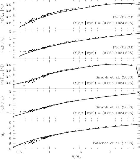
Figure 17: Masses of 92 high-fidelity members (§9.4.5), excluding the giants $\epsilon$ and $\gamma$ Tau. The most massive stars in this figure are (in order of decreasing mass): HIP 20894 A ($\theta^{2}$ Tau A; Appendix B.3), 20635, and 23497. Top two panels: the solid lines denote the effective temperature– and luminosity–stellar mass relations of the $(Y,Z)$$=$$(0.260,0.024)$ $625$ Myr CESAM isochrone (P98; §9.2). Third and fourth panels: as the top two panels, but for the $(Y,Z)$$=$$(0.285,0.024)$ $625$ Myr Padova isochrone (Girardi et al. 2000a). Bottom panel: the empirical absolute magnitude–mass relation of Patience et al. (1998) compared with the P98 stellar masses. The absolute magnitudes are based on Hipparcos secular parallaxes (§5).

10 Hertzsprung–Russell diagram

Figure 18 shows 92 high-fidelity Hyades (§9.3) with Padova and CESAM isochrones (§9.2) in the theoretical HR diagram (panel a) and the $\log T_{\rm eff}$–$\log g$ diagram (panel b). We used calibration (1) for the 14 evolved stars in the cluster turn-off region ($(B-V)\leq 0.30$ mag; $T_{\rm eff}\geq 7250$ K; §9.4.2) and calibration (2) for the remaining 76 dwarfs ($(B-V)>0.30$ mag; $T_{\rm eff}<7250$ K; §§9.4.3–9.4.4).

10.1 Low-mass main sequence ($M\mathrel{{\hbox to0.0pt{\lower 3.0pt\hbox{$\sim$}\hss}}\raise 2.0pt\hbox{$<$}}0.9\leavevmode\nobreak\ M_{\odot}$)

Figure 18: panel (a). HR diagram for 92 high-fidelity Hyades (§9.3). The stellar luminosities and effective temperatures were derived from secular parallax-based absolute magnitudes $M_{V}$ and $(B-V)$ colours using calibration (1) for $(B-V)\leq 0.300$ mag ($T_{\rm eff}\geq 7250$ K; 14 stars; §9.4.2) and calibration (2) for $(B-V)>0.300$ mag ($T_{\rm eff}<7250$ K; 76 dwarfs; §9.4.3). The giants $\gamma$ and $\epsilon$ Tau (HIP 20205 and 20889) are discussed in Appendix B.1; the components of the ‘resolved spectroscopic binary’ $\theta^{2}$ Tau (HIP 20894) are discussed in Appendix B.3. The lines labeled ‘1’, ‘2’, and ‘3’ are CESAM and Padova isochrones for the Hyades with Helium content $Y$, metal content $Z$, and age $\tau$ as indicated in the box (§9.2). The position of the Sun is indicated by $\odot$. The deviant locations of cool stars ($T_{\rm eff}\la 5000$ K) are a result of systematic errors in the $(B-V)$–$T_{\rm eff}$ calibrations (§10.1; cf. Figure 15). The inset shows the remaining members in the upper main sequence and turn-off region of the cluster (excluding HIP 21459, which has large photometric errors). HIP 20648 is discussed in §10.3. Deviant locations can be attributed to multiplicity, peculiar spectra, rotation, and/or suspect secular parallaxes ($g_{\rm Hip}>9$; Table 4).

Figure 18(a) shows, besides an inconsistency between the Padova and CESAM isochrones themselves, a significant discrepancy between the isochrones on the one hand and the inferred effective temperatures and luminosities for stars with $T_{\rm eff}\la 5000$ K (K/M dwarfs) on the other hand. As the ‘turn-off’ of the lower masses is absent in the colour-absolute magnitude diagram (Figure 13), we conclude that the model-observation discrepancies for these cool stars are caused by inappropriate $(B-V)$–$T_{\rm eff}$ calibrations (e.g., Gratton et al. 1996; cf. §9.4.1 and 9.4.4, Figures 17–16, and footnote 15). Reliable transformations for low-mass dwarfs with cool envelopes (or completely convective interiors) require non-gray non-LTE line-blanketed model atmospheres with appropriate molecular opacities (e.g., TiO, H₂O, and VO; e.g., Hauschildt et al. 1999). Theoretical models in this mass range similarly require adequate boundary conditions (Chabrier & Baraffe 1997). These models, for $M\la 0.6\leavevmode\nobreak\ M_{\odot}$, also suffer from uncertainties related to the equation of state, and, for $4000\la T_{\rm eff}\la 5000$ K, from uncertainties related to the treatment of convection (e.g., Ludwig et al. 1999).

Figure 18: panel (b). The $\log T_{\rm eff}$–$\log g$ diagram for the same 92 stars as in panel (a), but excluding the giants $\gamma$ and $\epsilon$ Tau. The line labeled ‘4’ denotes the BaSeL calibration main sequence for $[{\rm Fe/H}]=+0.14$ ($Z=0.024$; §9.4.3). Bessell et al.’s (1998) calibration (§9.4.2) is differently organized and cannot be plotted in this diagram.

The low-mass stars as a set show an enhanced spread about the main sequence compared to the higher mass stars. This effect is partly related to the degradation of secular parallax (i.e., Hipparcos proper motion) accuracies with $V$ magnitude. Part of the scatter might also be due to spectral peculiarities (e.g., emission lines as in HIP 20527 [K5.5Ve], 20605 [M0.5Ve], and 21138 [K5Ve]) or colour anomalies related to chromospheric activity (e.g., Campbell 1984; Stauffer et al. 1991, 1997); a 5 per cent starspot coverage yields $\sim$0.015 mag shifts in $(B-V)$, either towards the blue or towards the red, as well as low-level photometric variations (on the order of a few hundredths of a magnitude).

10.2 Intermediate-mass main sequence ($0.9\mathrel{{\hbox to0.0pt{\lower 3.0pt\hbox{$\sim$}\hss}}\raise 2.0pt\hbox{$<$}}M\mathrel{{\hbox to0.0pt{\lower 3.0pt\hbox{$\sim$}\hss}}\raise 2.0pt\hbox{$<$}}1.6\leavevmode\nobreak\ M_{\odot}$)

This mass range corresponds to F and G stars ($7500\ga T_{\rm eff}\ga 5000$ K). We divide it into three regimes corresponding to different interiors: (1) Stars with $M\ga 1.5\leavevmode\nobreak\ M_{\odot}$ ($B-V\la 0.30$ mag; $T_{\rm eff}\ga 7000$ K) have a convective core and radiative envelope. (2) With decreasing mass in the range $1.5\ga M\ga 1.3$–$1.1\leavevmode\nobreak\ M_{\odot}$ ($0.30\la B-V\la 0.40$ mag; $7000\ga T_{\rm eff}\ga 6500$–$6000$ K), the convective core shrinks to become radiative, while a convective envelope develops at the same time. This envelope gives rise to the formation of a chromosphere and corona. (3) Stars with $M\la 1.3$–$1.1\leavevmode\nobreak\ M_{\odot}$ ($B-V\ga 0.40$ mag; $T_{\rm eff}\la 6500$–$6000$ K) have a radiative core and convective envelope. Theoretical modelling for these regimes suffers mainly from uncertainties related to convection, notably overshoot of the core and envelope, and the issue of the universality of the mixing-length parameter $\alpha_{\rm MLT}$ (e.g., Ludwig et al. 1999; §9.1).

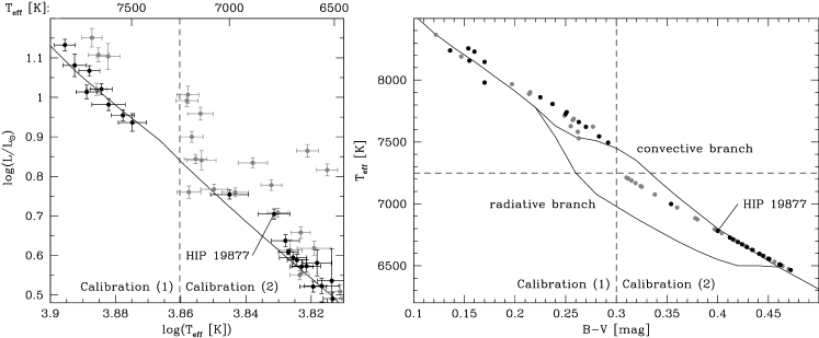
Figure 19: Left: HR diagram of the region of the onset of surface convection (the Böhm–Vitense gap; §10.2). The solid line denotes the 625 Myr CESAM isochrone. Black symbols show high-fidelity members; gray symbols denote remaining members (excluding HIP 21459, which has large photometric errors). Although the rotational velocity of the deviant object HIP 19877 (F5var) is unknown, its detection in X-rays (Hünsch et al. 1998) suggests the star has a convective envelope. Patience et al. (1998) did not detect a speckle companion. Its location above the main sequence is hence possibly related to stellar variability ($\Delta V\sim 0.07$ mag) or activity. The dashed line denotes $(B-V)=0.30$ mag ($T_{\rm eff}\sim 7250$ K), which marks the boundary between effective temperatures derived using calibrations (1) and (2) (§§9.4.2–9.4.3). Right: effective temperatures versus $(B-V)$ colours for the same set of stars as shown in the left panel. The dashed horizontal line denotes $T_{\rm eff}=7250$ K, and is shown for reference. The solid line shows the Böhm–Vitense (1981) Solar-metallicity $(B-V)$–$T_{\rm eff}$ relation; the bifurcation into radiative and convective branches is discussed in §10.2.

Figure 18(a) shows that the effective temperatures and luminosities closely follow the CESAM isochrone, except in the range $7000\ga T_{\rm eff}\ga 6500$ K ($0.30\la(B-V)\la 0.40$ mag) where the observations are suggestive of a ‘turn-off’ of the main sequence around spectral type $\sim$F5V. Figure 19 shows an expanded view of this region, including the locations of all non-high-fidelity members. The ‘turn-off’ is also clearly visible in the secular parallax-based colour-absolute magnitude diagrams displayed in Figures 11 and 13. We therefore conclude that it is not caused by the $(B-V)$–$T_{\rm eff}$ relation adopted in this study (§9.4.4; cf. Figure 16; we do note, however, that the ‘turn-off’ roughly coincides with the transition at $(B-V)=0.30$ mag ($T_{\rm eff}\sim 7250$ K) between calibration (1) (§9.4.2) and calibration (2) (§9.4.3)). We suspect, as argued below, that the ‘turn-off’ is related to the onset of surface convection around $(B-V)=0.30$–$0.40$ mag (cf. de Bruijne et al. 2000). This is consistent with the work of Rachford (1997, 1998), who detected a transition in stellar activity parameters at $(B-V)\sim 0.29$ mag as well as a chromospherically active Hyad at $(B-V)=0.26$ mag (HIP 21036). These findings indicate that the onset of convection (in the Hyades) occurs at $(B-V)\ga 0.25$–$0.30$ mag (cf. Wolff et al. 1986; Rachford & Canterna 2000).

Böhm–Vitense (1970, 1981, 1982) first realized that convective atmospheres have relatively low temperatures in the deeper layers which contribute to the surface flux in the spectral regions of the $U$ and $B$ filters (cf. Nelson 1980). As a result, convective atmospheres have reddened $(B-V)$ colours (as compared to radiative atmospheres of the same $T_{\rm eff}$) by amounts of $\sim$0.07–0.12 mag. As the reddening of the atmosphere is not accompanied by a significant change in luminosity, the onset of surface convection can cause a $\sim$$0.10$ mag ‘gap’ and/or ‘turn-off’ in the $(B-V)$ colour-absolute magnitude diagram, starting around $(B-V)=0.25$–$0.35$ mag, the so-called Böhm–Vitense gap (cf. figure 2 in de Bruijne et al. 2000). Observational evidence for the existence of the Böhm–Vitense gap is sparse (e.g., Böhm–Vitense & Canterna 1974; Jasniewicz 1984; Rachford & Canterna 2000), and its reality has been disputed (e.g., Mazzei & Pigatto 1988; Simon & Landsman 1997; Newberg & Yanny 1998). Previous claims for its existence were based on the presence of gaps in either colour-colour diagrams or in the cumulative distribution of cluster members in some photometric index (e.g., Aizenman et al. 1969), instead of on the presence of ‘gaps’ or ‘turn-offs’ in colour-absolute magnitude diagrams. The secular parallax-based colour-absolute magnitude diagrams of the Hyades presented in Figures 11 and 13 provide, in fact, the first direct evidence in favor of the existence of the Böhm–Vitense gap.

Table 4: Some remaining stars in the upper main sequence and turn-off region of the Hyades. Spectroscopic binarity (‘SB’; table 2 in P98), high rotational velocities ($v\sin i$ from Abt & Morrell 1995; km s^-1), suspect secular parallaxes ($g_{\rm Hip}>9$), and spectral peculiarities can give rise to deviant HR diagram positions. Hipparcos field H52 is a photometric variability flag (‘M’ for micro-variable). The symbol $\delta$ Sct stands for $\delta$ Scuti pulsator.

HIP	SB	$v\sin i$	Notes	HIP	SB	$v\sin i$	Notes	HIP	SB	$v\sin i$	Notes
20400	SB	25	Am; $\delta$ Sct	2090		93	Am	21683c		115	$g_{\rm Hip}=11.92$; A5Vn
20484	SB	15	Am	2103	SB	31	Am	22157	SB	63	Am; $g_{\rm Hip}=23.34$
20614a		145		2127	SB	130		22565		165	H52 = ‘M’; $\delta$ Sct
20711		225	H52 = ‘M’; $\delta$ Sct; A8Vn	2158	SB	78		23983	SB	13	Am
20713b	SB	205	$g_{\rm Hip}=30.30$; $\delta$ Sct	2167		75	Am	24019d		45	Am

^a: Eggen’s (1992) ‘photometry indicates a possible binary, which is not resolved by speckle observations’. Patience et al. (1998) did not detect a speckle companion. Wielen et al. (2000) list the star as ‘$\Delta\mu$ binary’.
^b: A chromospherically active long-period F0V+G4V binary (Peterson et al. 1981); the object is the second-brightest X-ray source in the Hyades (e.g., Stern et al. 1992, 1994).
^c: Parallaxes differ significantly ($\pi_{\rm Hip}=20.51\pm 0.82$, $\pi_{\rm sec,Hip}=18.33\pm 0.42$, $\pi_{\rm sec,Tycho-2}=18.70\pm 0.38$ mas; $g_{\rm Hip\-/Tycho-2}=$ $11.92\-/8.74$), possibly as a result of multiplicity. Patience et al. (1998) did not detect a speckle companion.
^d: Primary target of a two-pointing system (field H60 = ‘P’); the A component is a periodic variable. The secondary target is HIP 24020; the double star processing used a linear system (H60 = ‘L’): the parallax of the B component is constrained to be identical to the A-component parallax, whereas the proper motions were independently determined. The solution is uncertain (H61 = ‘D’). HIP 24020 is a duplicity-induced variable (H52 = ‘D’); the B component itself is a resolved Hipparcos binary.

A careful inspection of Figures 11, 13, and 18(a) reveals that the region around $(B-V)\sim 0.45$ mag ($T_{\rm eff}\sim 6400$ K) also shows an abrupt increase in the $(B-V)$ colours of stars by an amount of $\sim$0.05 mag. This feature was already commented on by Böhm–Vitense (1995a, b), who attributed it to ‘a sudden increase in convection zone depths’. The position of the second Böhm–Vitense gap coincides with both the so-called Lithium gap, which is generally thought to be related to the rapid growth of the depth of the surface convection zone with effective temperature decreasing from $\sim$7000 K to $\sim$6400 K (e.g., Boesgaard & Tripicco 1986; Michaud 1986; Swenson et al. 1994; Balachandran 1995), and the onset of dynamo-induced magnetic chromospheric activity (cf. Wolff et al. 1986; García Lopéz et al. 1993).

As stellar rotation is known to influence significantly the precise conditions for the onset of surface convection (e.g., Chandrasekhar 1961), Böhm–Vitense suggested that a range of $v\sin i$ values within a stellar cluster can lead to a bifurcation of the $(B-V)$–$T_{\rm eff}$ relation in the range $6500\la T_{\rm eff}\la 7500$ K (cf. Simon & Landsman 1997). This means that a star with a given $(B-V)$ colour can be either a slowly rotating weakly convective star with a ‘high’ effective temperature or a rapidly rotating radiative star with a ‘lower’ effective temperature, where the ‘high’ and ‘low’ temperatures can differ by as much as 500 K. The righthand panel of Figure 19 compares Böhm–Vitense’s (1981; her table 3 and figure 4) predictions of the two branches to the effective temperatures derived using calibrations (1) and (2) (§§9.4.2–9.4.3). The calibration (1) and (2) effective temperatures do not show a bifurcation, simply because they do not take stellar rotation into account. Systematic differences outside the bifurcation region can be due to the presently outdated Solar-metallicity atmosphere models used by Böhm–Vitense in 1981. A natural next step would be to determine, for each Hyades member in the region of the (first) Böhm–Vitense gap, its rotational velocity, to determine its effective temperature based on adequate stellar modelling, i.e., taking stellar rotation into account, and to compare the resulting location in the $T_{\rm eff}$–$(B-V)$ diagram (Figure 19) with the predictions of Böhm–Vitense (1981).

Naively, one would expect that the peculiar $(B-V)$ behaviour resulting from (the onset of) surface convection is incorporated in the (synthetic) $(B-V)$–$T_{\rm eff}$ relations adopted in this paper. However, as the onset of surface convection is a subtle effect when translated into the mass range at stake, its visibility in the theoretical HR diagram (Figure 18(a)) is probably the result of an inappropriate mass sampling in the construction of the synthetic $(B-V)$–$T_{\rm eff}$ relations (§§9.4.2–9.4.3). Only a future investigation of the interplay between stellar rotation and (the onset of) surface convection, and the corresponding effects on the atmospheric parameters of mid-F stars (e.g., Hartmann & Noyes 1987; Chaboyer et al. 1995), can shed more light on the issue of the ‘turn-off(s)’ of the Hyades main sequence and the bifurcation of the $(B-V)$–$T_{\rm eff}$ relation.

10.3 The upper main sequence and turn-off region ($M\mathrel{{\hbox to0.0pt{\lower 3.0pt\hbox{$\sim$}\hss}}\raise 2.0pt\hbox{$>$}}1.6\leavevmode\nobreak\ M_{\odot}$)

Beyond $T_{\rm eff}\ga 7500$ K, we find the early-F and late-A stars which are evolving towards the end of the core Hydrogen burning phase. These objects are powered by the CNO-cycle and have convective cores and radiative envelopes. As a result, the precise locations of the isochrones depend strongly on the treatment of rotationally-induced mixing (Maeder & Meynet 2000) and the amount of convective core overshoot included in the models (e.g., §9.2 in P98). Given these uncertainties, Figure 18 shows that the stars on the upper main sequence of the Hyades follow the 625–650 Myr CESAM isochrones (including convective core overshoot) remarkably well, both in luminosity (panel a) and in surface gravity (panel b).

Many stars in the turn-off region of the Hyades rotate rapidly (e.g., table 11 in P98). Stellar rotation influences the observed colours and magnitudes (and thus the inferred temperatures and luminosities) of stars, the amounts depending on the rotation characteristics (solid-body or differential rotation), the rate of rotation, the orientation of the rotation axis with respect to the observer, and the spectral type of the star (e.g., Kraft & Wrubel 1965; Maeder & Peytremann 1970, 1972; Collins & Smith 1985; Pérez Hernández et al. 1999; Maeder & Meynet 2000). Although the photometric effect of rotation also depends on the specific filter system in use, rotating stars generally become redder (typically a few hundredths of a magnitude in $(B-V)$; $\sim$200–250 K in $T_{\rm eff}$) as well as brighter or fainter (typically a few tenths of a magnitude in $V$). An example of a rapidly rotating star in the Hyades turn-off region is HIP 23497 ($v\sin i\sim 126$ km s^-1; $\log(T_{\rm eff}[{\rm K}])=3.9115$; $\log(L/L_{\odot})=1.472$); its deviant location in the HR diagram is most likely due to rotation: although the object is listed as equal-magnitude occultation double by Hoffleit & Jaschek (1991), Patience et al. (1998) did not detect a secondary.

The turn-off region of the Hyades coincides with the lower part of the instability strip (e.g., Liu et al. 1997). Some of the stars accordingly pulsate (e.g., Antonello & Pasinetti Fracassini 1998). An example is the primary component of the ‘resolved spectroscopic binary’ $\theta^{2}$ Tau (HIP 20894), which is a $\delta$ Scuti pulsator (e.g., Breger et al. 1987, 1989; Kennelly et al. 1996; cf. Appendix B.3 and Table 3). The A7III–IV primary has an A5V secondary. The exact location of both stars in the turn-off region of the HR diagram therefore puts a severe constraint on stellar evolutionary models of the system as well as of the Hyades cluster (e.g., Lastennet et al. 1999). Unfortunately, the precise evolutionary status of the evolved component is unknown. Moreover, observations as well as theoretical modelling are complicated by the fact that both stars, which are roughly equally bright, are rapid rotators ($[v\sin i]_{\rm primary}\sim 80$ km ^-1; $[v\sin i]_{\rm secondary}\ga 90$ km ^-1), resulting in severely blended spectra.

The secular parallax of the binary allows to position both components in the HR diagram with unprecedented precision. Figure 18(a) suggests that $\theta^{2}$ Tau A is close to the end of the core Hydrogen burning phase, and is about to undergo an overall gravitational contraction which will ignite thick Hydrogen shell burning. This is consistent with the low amplitude of the pulsations, indicative of main sequence evolution (e.g., Li & Michel 1999; large-amplitude pulsators (0.10 mag or higher) are thought to be evolved stars in the Hydrogen shell burning phase). These results confirm the conclusion of Torres et al. (1997c), which was based on the orbital parallax of the binary (Table 3), but are in conflict with Królikowska’s (1992) finding that $\theta^{2}$ Tau A currently burns Hydrogen in a thick shell.

The bluest Hyad is HIP 20648 (A2IVm; $(B-V)=0.049\pm 0.007$ mag). Being a Hipparcos duplicity-induced variable (field H52 is ‘D’) and component binary (H59 is ‘C’; $\Delta Hp=4.02\pm 0.09$ mag), the object is not included in our high-fidelity sample. Nonetheless, the object is a secure member of the Hyades: its secular parallax solution (based on the Hipparcos A-component proper motion; H10 is ‘A’) is of high quality ($g_{\rm Hip}=0.46$), and the observed radial velocity and parallax (secular as well as trigonometric) are consistent with membership (e.g., table 2 in P98). Applying calibration (1) to the observed colour and secular parallax returns $\log(T_{\rm eff}[{\rm K}])=3.9649\pm 0.0061$ and $\log(L/L_{\odot})=1.541\pm 0.017$. These parameters put the star on the Hyades main sequence, but far beyond the turn-off (inset of Figure 18(a)). This ‘blue straggler’ nature is not readily explained by rapid rotation (since $v\sin i=15$ km s^-1 and a pole-on orientation is unlikely) or an inappropriate calibration (e.g., Burkhart & Coupry (1989) found $T_{\rm eff}=9050\pm 100$ K). The observation of a large photospheric (and thus presumably also large interior) magnetic field (Babcock 1958) suggests that the apparently prolonged hydrogen core burning phase of this star, as compared to other members of similar mass which have already evolved off the main sequence, can be explained if the Helium produced in the core is continuously replaced with fresh Hydrogen through large-scale magnetic mixing (e.g., Hubbard & Dearborn 1980; Abt 1985).

The inset of Figure 18(a) shows all objects in the turn-off region of the Hyades which are not contained in the objectively defined sample of high-fidelity members (cf. Table 4). The deviant HR diagram locations of some of these members are most likely caused by: (1) suspect secular parallaxes (i.e., $g_{\rm Hip}>9$); (2) stellar rotation; (3) (spectroscopic) binarity; or (4) an inappropriate calibration (§9.4). The latter option might be especially relevant for the slowly rotating metallic-line A stars. Uncertainties in (metal-)line-blanketing, line lists, and opacities in atmosphere models, the treatment of the diffusion of chemical elements, and the treatment of large-scale motions in the envelopes of these stars give rise to significant uncertainties in the $T_{\rm eff}$-scale (e.g., Smalley & Dworetsky 1993; Richer et al. 2000).

10.4 The giant region

The red clump of the Hyades contains four giants: $\theta^{1}$, $\delta^{1}$, $\epsilon$, and $\gamma$ Tau; the determination of their effective temperatures and secular parallax-based luminosities is discussed in Appendices B.1–B.2 Whereas $\epsilon$ and $\gamma$ Tau are single stars, $\theta^{1}$ and $\delta^{1}$ Tau are spectroscopic binaries. The secular parallaxes of these double stars should be treated with care as they could be based on astrometric data which do not properly reflect their true space motions (§4.3).

Figure 20: The Hyades red giant clump based on Hipparcos secular parallaxes (Appendices B.1–B.2). The solid line denotes Girardi et al.’s (2000a) $(Y,Z)=(0.273,0.019)$ 631 Myr isochrone. The objects $\delta^{1}$ and $\theta^{1}$ Tau are spectroscopic binaries; their secular parallaxes and luminosities should be treated with care (§10.4). The ‘suspected non-single’ K2III giant $\delta$ Ari is not coeval with the Hyades; this conclusion does not depend on the suspect secular parallax of the star (§10.4).

The location of isochrones in the giant region not only depends quite sensitively on metallicity but also on the mass loss history on the red giant branch and the adopted value of the mixing-length parameter $\alpha_{\rm MLT}$. Nonetheless, all Hyades giants precisely follow Girardi et al.’s (2000a) Solar-metallicity 631 Myr isochrone (§9.2; Figure 20), despite the fact that Girardi simply accounted for mass loss by means of Reimers’ (1975) empirical formula (using a mass-loss efficiency parameter of $0.4$; Renzini & Fusi Pecci 1988). A natural next step would be to investigate the variation of the location of the red giant clump with metallicity, mass loss, and mixing-length parameter (cf. Girardi et al. 2000b). Such an analysis would give, e.g., more insight into the reliability of red clump giants as distance calibrators (e.g., Alves 2000; Udalski 2000).

The P98 member list contains one additional evolved star of spectral type K2III. This object ($\delta$ Ari; HIP 14838; Appendix B.2) has several characteristics of a non-member: it is located $15.34$ pc from the cluster center, it has a near-Solar metallicity as opposed to the mean Hyades value $[{\rm Fe/H}]=+0.14\pm 0.05$, it has an unreliable secular parallax solution, and it was rejected by de Bruijne (1999a) and Hoogerwerf & Aguilar (1999) as proper motion member of the Hyades (Table LABEL:tab:data_1). Although the latter two facts could be spurious due to possible duplicity (Appendix B.2; Wielen et al. 2000), Figure 20 shows that $\delta$ Ari is not coeval with the classical giants in the cluster. We conclude that the star is most likely a non-member.

10.5 White dwarfs

The Hyades contains a dozen known white dwarfs (e.g., Humason & Zwicky 1947; Luyten 1954, 1956; Böhm–Vitense 1995). They typically have $V\ga 14$ mag, which means they are too faint to be observed directly by Hipparcos. However, several white dwarfs are contained in multiple systems (e.g., Lanning & Pesch 1981), the primary components of which were observed by Hipparcos. We discuss two of such systems.

V471 Tau:

HIP 17962 is a post-common-envelope detached eclipsing binary. It is composed of a DA white dwarf and a coronally active K2V star. Hosting the hottest and youngest Hyades white dwarf, V471 Tau has been studied extensively (e.g., Nelson & Young 1970, 1972; Guinan & Sion 1984; Clemens et al. 1992; Shipman et al. 1995; Marsh et al. 1997). The system is a pre-cataclysmic variable: the K star does not fill its Roche lobe yet. The observed periodic optical and X-ray variations are related to material from the K-star wind being accreted onto the magnetic poles of the rotating white dwarf (e.g., Jensen et al. 1986; Barstow et al. 1992).

Table 5: Fundamental parameters of two Hyades white dwarfs. V471 Tau: effective temperatures and surface gravities determined from ORFEUS/IUE spectra (Barstow et al. 1997; Werner & Rauch 1997). The orbital elements of the eclipsing binary imply a mass function of $0.174\pm 0.002\leavevmode\nobreak\ M_{\odot}$; using $80^{\circ}\!\leq i\leq 90^{\circ}\!$ returns an astrometric white dwarf mass $M=0.759\pm 0.020\leavevmode\nobreak\ M_{\odot}$ for an assumed K-dwarf mass $M=0.800\leavevmode\nobreak\ M_{\odot}$ (Young 1976; Bois et al. 1988). The white dwarf radius $R$ is independently determined from model fluxes and the observed parallax and flux. The inferred surface gravity then follows from combining this radius with the astrometric mass. Barstow et al. used Wood’s (1995) evolutionary models to derive a spectroscopic mass $M/M_{\odot}=0.61^{+0.14}_{-0.10}$ and radius $R/R_{\odot}=0.014\pm 0.003$. ‘This study’ combines the secular parallax of V471 Tau with Werner & Rauch’s model. HD 27483: results from Böhm–Vitense (1993) and Burleigh et al. (1998). The Burleigh et al. and ‘This study’ results were derived from an interpolation in Burleigh’s table 5 using the Hipparcos trigonometric and secular parallax, respectively. Burleigh et al. themselves quote $\log g=8.5$, $T_{\rm eff}=2\,2000$ K, and $M/M_{\odot}=0.94$.

V471 Tau	Barstow et al.	Werner & Rauch	This study
HIP 17962	(1997; $\pi_{\rm Hip}$)	(1997; $\pi_{\rm Hip}$)	($\pi_{\rm sec,Hip}$)
$T_{\rm eff}[{\rm K}]$ (spectroscopic)	$32\,400^{+270}_{-800}$	35 125$\pm$1275
$\log(g[{\rm cm\leavevmode\nobreak\ s}^{-2}])$ (spectroscopic)	$8.16^{+0.18}_{-0.24}$	8.21$\pm$0.23
$M/M_{\odot}$ (from orbit)	0.76$\pm$0.02	0.759$\pm$0.020	0.759$\pm$0.020
$R/R_{\odot}$ (from parallax)	0.0107$\pm$0.0009	0.0097$\pm$0.0013	0.0098$\pm$0.0011
$\log(g[{\rm cm\leavevmode\nobreak\ s}^{-2}])$ (inferred)	8.27$\pm$0.07	8.35$\pm$0.12	8.34$\pm$0.10
HD 27483	Böhm–Vitense	Burleigh et al.	This study
HIP 20284	(1993; $\pi_{\rm sec,Schwan\leavevmode\nobreak\ (1991)}$)	(1998; $\pi_{\rm Hip}$)	($\pi_{\rm sec,Hip}$)
$T_{\rm eff}[{\rm K}]$	$23\,800$	$21\,815\pm 178$	$21\,555\pm 84$
$\log(g[{\rm cm\leavevmode\nobreak\ s}^{-2}])$	8.03	$8.34\pm 0.16$	$8.11\pm 0.07$
$M/M_{\odot}$	0.60	$0.84\pm 0.10$	$0.696\pm 0.041$
$R/R_{\odot}$	0.012	$0.010\pm 0.002$	$0.0121\pm 0.0006$

The effective temperature and surface gravity of the white dwarf in V471 Tau were recently determined by fitting synthetic spectra to observed spectra of the Hydrogen Lyman lines (Barstow et al. 1997; Werner & Rauch 1997; Table 5). Unfortunately, the relatively large uncertainty in the best-fit $\log g$ values prevents an accurate mass determination. It has therefore been common practice to infer the surface gravity of the white dwarf from its astrometric mass, obtained from the orbital elements of the binary, and its radius, obtained from its observed and modelled flux combined with its Hipparcos parallax (Table 5).

A more precise estimate of the white dwarf radius is available through its secular parallax. The latter is non-suspect ($g_{\rm Hip}=0.06$), and fully consistent with the Hipparcos parallax ($\pi_{\rm Hip}=21.37\pm 1.62$ mas; $\pi_{\rm sec,Hip}=21.00\pm 0.40$ mas). The long time-baseline Tycho–2 secular parallax, which might be preferred over the Hipparcos secular parallax in view of the binary nature of the system (although $P_{\rm orb}=0.521$ days only; Stefanik & Latham 1992; §4.3), places the object at a slightly, though not significantly, larger distance ($\pi_{\rm sec,Tycho-2}=20.56\pm 0.33$ mas with $g_{\rm Tycho-2}=0.02$). The Hipparcos secular parallax fits Werner & Rauch’s (1997) model for a radius of $R/R_{\odot}=0.0098\pm 0.0011$; the corresponding surface gravity is $\log g=8.34\pm 0.10$ for $M/M_{\odot}=0.759\pm 0.020$ (Table 5). These values are fully consistent with but (in principle) more precise than the results of Werner & Rauch (1997) and Barstow et al. (1997).

HD 27483: In 1993, Böhm–Vitense reported the serendipitous discovery of a DA white dwarf companion around the close F6V–plus–F6V binary HD 27483 (HIP 20284). Böhm–Vitense interpreted her spectra using Wesemael et al.’s (1980) unblanketed white dwarf models and Hamada & Salpeter’s (1961) mass–radius relation, assuming a distance to the system of 47.6 pc (the secular parallax derived by Schwan 1991; Table 5). Recently, Burleigh et al. (1998) presented an analysis of the object, based on updated atmosphere and evolutionary models (Koester 1991; Wood 1995), using its Hipparcos parallax ($\pi_{\rm Hip}=21.80\pm 0.85$ mas). The orbital motion of the binary ($P_{\rm orb}=3.05$ days; Mayor & Mazeh 1987) has not hampered the Hipparcos measurements: its secular parallax ($\pi_{\rm sec,Hip}=20.59\pm 0.35$ mas) is well defined ($g_{\rm Hip}=2.73$). We use cubic spline interpolation in Burleigh’s table 5 to derive $\log g$, $T_{\rm eff}$, $M$, and $R$ for both the Hipparcos trigonometric and secular parallaxes (Table 5). The secular parallax-based white dwarf mass ($M/M_{\odot}=0.70\pm 0.04$) is significantly smaller than Burleigh et al.’s value ($M/M_{\odot}=0.94$). The new mass estimate resolves the problem (acknowledged by Burleigh et al.) that the sum of the cooling age of a $M=0.94\leavevmode\nobreak\ M_{\odot}$ white dwarf and the evolutionary age of its progenitor is significantly shorter than the nuclear age of the Hyades.

11 Summary and discussion

At $\sim$45 pc, the Hyades is the nearest open cluster to the Sun. Its tidal radius of $\sim$10 pc translates to an angular extent of several tens of degrees on the sky and to a significant line-of-sight extension compared to its mean distance. Hipparcos trigonometric parallaxes, with typical accuracies of $\sim$1.5 mas, constrain the positions of members in the cluster to within a few parsec. Although this precision is sufficient to study the three-dimensional structure of the cluster, and related issues like mass segregation. uncertainties in the ‘trigonometric distances’ to individual stars dominate the error budget when constructing the colour-absolute magnitude diagram of the cluster. The considerable tangential velocity of the cluster (relative to the Sun) opens the possibility to derive parallaxes for individual stars from their measured proper motions (§5). Despite the presence of an internal velocity dispersion in the cluster of $\sim$0.30 km s^-1 (in one dimension), the proper motion-based (secular) parallaxes are $\sim$3 times more precise than the Hipparcos trigonometric values (§5.4).

The secular parallaxes are derived under the assumption that all cluster stars follow a three-dimensional Gaussian velocity distribution with an isotropic dispersion (§3). A careful analysis confirms the absence of significant velocity structure in the form of expansion, rotation, or shear (§6). Numerical and theoretical work suggests that members beyond the tidal radius of the cluster (the halo and moving group population) (may) have a systematically different velocity field from the main body of the cluster (the core and corona). We show that the maximum expected systematic secular parallax errors in the outer regions of the cluster are $\la$0.30 mas (§6.5), i.e., a factor $\sim$2 smaller than typical random secular parallax errors. The Hipparcos trigonometric and secular parallaxes as a set are statistically fully consistent. Nonetheless, we do find evidence for the presence of spatially correlated Hipparcos measurements on small angular scales (i.e., a few degrees), consistent with the predictions of the Hipparcos data reduction consortia (§6.2). The maximum ‘amplitude’ of the correlation is $\la$$0.50$–$0.75\sigma\sim 0.75$–$1.00$ mas per star, which is a factor of $\sim$2 smaller than the value quoted by Narayanan & Gould (1999b).

Our list of Hyades candidate members contains 233 stars (§4). These are the 218 candidates selected by P98 and 15 new Hipparcos stars selected by de Bruijne’s (1999a) and/or Hoogerwerf & Aguilar’s (1999) methods. Only one of the latter stars (HIP 19757) is a likely member (§5.2). Long time-baseline Tycho–2 proper motions are available for (most of) the brighter Hyades that were observed by Hipparcos; the corresponding secular parallaxes are fully consistent with both the Hipparcos trigonometric and the Hipparcos secular parallaxes.

The secular parallaxes for members of the Hyades allow the construction of the most precise colour–absolute magnitude diagram of the cluster to date (Figures 10 and 13; see also, e.g., Madsen 1999). The main sequence is well defined, and shows a few conspicuous but artificial gaps, e.g., around $(B-V)=0.95$ and between $(B-V)=0.30$ and $(B-V)=0.35$ mag, caused by the suppression of (double and multiple) stars from our sample (cf. figure 21 of P98). The small gap between $(B-V)=0.75$ and $0.80$ mag is also present in the original sample and is therefore probably real (cf. figure 2 of Mermilliod 1981). Somewhat further to the blue, there are two conspicuous features (‘gaps’ and/or ‘turn-offs’) around $(B-V)\sim 0.30$ ($T_{\rm eff}\sim 7000$ K) and $\sim$0.45 mag ($\sim$$6400$ K). These features, which have never been observed this clearly before, but the existence of which was predicted by E. Böhm–Vitense already $\sim$30 years ago, are related to the use of the $(B-V)$ colour as temperature indicator. We suspect, following Böhm–Vitense, that sudden changes in the properties of surface convection zones in the atmospheres of stars with $(B-V)\sim 0.30$ and $\sim$0.45 mag significantly affect the emergent UV and blue-optical fluxes, and thus the $(U-B)$ and $(B-V)$ colours (§10.2).

As the Hipparcos members of the Hyades span a large range in mass and occupy a number of different evolutionary states, their effective temperatures and luminosities provide stringent constraints on both the global characteristics of the Hyades (such as metallicity, Helium content, and age) and stellar evolutionary modelling in general (cf. Lebreton 2000). We combine the secular parallaxes derived in this study with two existing $(B-V)\longrightarrow\log T_{\rm eff}$ and $M_{V}\longrightarrow\log(L/L_{\odot})$ calibrations (§9.4) to infer the fundamental properties of the cluster as well as of a variety of members. The latter include, among others, stars with surface convection zones, Am stars, a $\delta$ Scuti pulsator, red giants, and white dwarfs (§10). We show that neither the Bessell et al. (1998) nor the Lejeune et al. (1998) $(B-V)$–$T_{\rm eff}$ and $T_{\rm eff}$–${\rm BC}_{V}$ calibrations (whether correcting for the non-Solar metallicity of the Hyades or not) are appropriate throughout the entire mass range studied in this paper; only an ad-hoc combination of the two calibrations provides an acceptable fit to the P98 CESAM isochrones.

An optimum exploitation of the secular parallax data requires several future steps. An obvious need is the construction of a set of isochrones that are based on homogeneous stellar evolutionary modelling, tailored to the Hyades cluster in terms of chemical composition and age, from the low-mass main sequence ($M\ga 0.50\leavevmode\nobreak\ M_{\odot}$) through the clump-giant region (§10.4). The lack of this information prevents us from validating the chemical composition and age of the cluster derived by P98. The precision with which the secular parallaxes constrain the locations of stars in the HR diagram brings out such detailed structure in the main sequence (e.g., the Böhm–Vitense gaps) that the construction of future isochrones will require a fine-tuned mass sampling as well as, for stars near the Böhm–Vitense gap, inclusion of stellar rotation (§10.2). This study has shown that the most significant uncertainty in the secular parallax-based HR diagram locations of stars is now set by systematic errors in the available transformations of the observed optical broad-band colours and absolute magnitudes to effective temperatures and luminosities (cf. Nordström et al. 1997; Castellani et al. 2000). This issue clearly requires future study, for which the secular parallaxes provide stringent boundary conditions.

An application of the secular parallax method to other nearby clusters, such as Coma Berenices, the Pleiades, and Praesepe, is feasible. Improved parallaxes can be obtained for these groups (cf. Dravins et al. 1999), although several complicating factors exist (as compared to the Hyades). Among these are their larger mean distances, smaller fields on the sky, less well-defined (Hipparcos) membership lists, and the presence of interstellar reddening and extinction. The secular parallaxes for the Hyades cluster presented in this paper will only be superseded by the measurements of a second generation of astrometric satellites, such as FAME, DIVA, and notably GAIA (http://aa.usno.navy.mil/fame/, www.- aip.de/groups/DIVA/, astro.estec.esa.nl/GAIA/).

Appendix A Data

Tables LABEL:tab:data_1–7 contain data for the 218 Hyades candidates selected by P98 (§4.1) and the 15 new candidates selected by de Bruijne (1999a) and Hoogerwerf & Aguilar (1999; §4.2), respectively. The fundamental stellar parameters listed in columns (10)–(13) of Table LABEL:tab:data_1 are based on the Hipparcos secular parallaxes, and the $V$ and $(B-V)$ values listed in the Hipparcos Catalogue (ESA 1997; fields H5 and H37, respectively; cf. §9.4).

Appendix B $(B-V)$–$M_{V}$ $\longrightarrow$ $\log T_{\rm eff}$–$\log(L/L_{\odot})$

B.1 The giants $\epsilon$ and $\gamma$ Tau

The Hyades cluster contains two single giants, $\epsilon$ Tau (HIP 20889) and $\gamma$ Tau (HIP 20205; §§9.3 and 10.4). Both stars are located in the giant clump, i.e., the core Helium burning phase. Table 6 shows the results of applying calibration (1) (§9.4.2) to $\epsilon$ and $\gamma$ Tau for $[{\rm Fe/H}]=0$ and $+0.14$ (although it formally applies to dwarfs only).

The effective temperatures, surface gravities, metallicities, and bolometric fluxes of $\epsilon$ and $\gamma$ Tau have recently been determined through combining the infra-red flux method with modelling of high-resolution spectra using MARCS model atmospheres (Table 6; Smith & Ruck 1997; Smith 1999). Luminosities for both stars can be obtained by combining their bolometric fluxes with parallaxes; results for Hipparcos trigonometric and secular parallaxes are listed in Table 6 under Smith & Ruck (1997) and Smith (1999), respectively. Although calibration (1) gives very similar results, we use the infra-red flux method temperatures and secular parallax-based luminosities.

B.2 The giants $\delta^{1}$ and $\theta^{1}$ Tau and $\delta$ Ari

Table 6: Fundamental properties of the single Hyades red giants (cf. table 2 in Smith & Ruck 1997). The luminosities $\log(L/L_{\odot})$ listed for Smith & Ruck (1997) and Smith (1999) were derived from combining integrated stellar fluxes above the Earth’s atmosphere determined using the infra-red flux method ($F_{\gamma\leavevmode\nobreak\ {\rm Tau}}=1.14\cdot 10^{-9}$ W m^-2; $F_{\epsilon\leavevmode\nobreak\ {\rm Tau}}=1.28\cdot 10^{-9}$ W m^-2; Blackwell & Lynas–Gray 1998) with Hipparcos trigonometric and secular parallaxes, respectively. The giant metallicities $[{\rm Fe/H}]=+0.14$ and masses $M/M_{\odot}=2.32\pm 0.10$ used in calibration (1) were taken from P98. These mass estimates are consistent with the clump giant masses of $\sim$$2.4\leavevmode\nobreak\ M_{\odot}$ listed by Torres et al. (1997a, c).

$\gamma$ Tau (K0III)	Smith & Ruck (1997)	Smith (1999)	Calibration (1)	Calibration (1)
HIP 20205	$L=L(\pi_{\rm Hip})$	$L=L(\pi_{\rm sec,Hip})$	$[{\rm Fe/H}]=+0.14$	$[{\rm Fe/H}]=0$
$\log(L/L_{\odot})$	$1.901\pm 0.016$	$1.869\pm 0.016$	$1.843\pm 0.016$	$1.850\pm 0.016$
$\log(T_{\rm eff}[{\rm K}])$a	$3.6959\pm 0.0035$		$3.7004\pm 0.0027$	$3.6967\pm 0.0027$
$\log(g[{\rm cm\leavevmode\nobreak\ s}^{-2}])$	$2.65\pm 0.20$	$2.63\pm 0.03$	$2.714\pm 0.027$	$2.692\pm 0.027$
$[{\rm Fe/H}]$c	$+0.12\pm 0.03$	$+0.150\pm 0.029$	$+0.14$	$+0.00$
$M/M_{\odot}$		$2.30\pm 0.10$	$2.32\pm 0.10$	$2.32\pm 0.10$
$\epsilon$ Tau (K0III)
HIP 20889
$\log(L/L_{\odot})$	$1.956\pm 0.015$	$1.927\pm 0.015$	$1.912\pm 0.015$	$1.919\pm 0.015$
$\log(T_{\rm eff}[{\rm K}])$b	$3.6912\pm 0.0031$		$3.6938\pm 0.0022$	$3.6902\pm 0.0022$
$\log(g[{\rm cm\leavevmode\nobreak\ s}^{-2}])$	$2.45\pm 0.20$	$2.57\pm 0.03$	$2.619\pm 0.026$	$2.598\pm 0.026$
$[{\rm Fe/H}]$c	$+0.15\pm 0.03$	$+0.163\pm 0.030$	$+0.14$	$+0.00$
$M/M_{\odot}$		$2.30\pm 0.10$	$2.32\pm 0.10$	$2.32\pm 0.10$
$T_{{\rm eff},\gamma\leavevmode\nobreak\ {\rm Tau}-\epsilon\leavevmode\nobreak\ {\rm Tau}}$ [K]	$+54\pm 53$	$+80\pm 20$	$+76\pm 40$	$+74\pm 40$

^a: $\log(T_{\rm eff}[{\rm K}])=3.6955\pm 0.0013$ (Taylor 1999).
^b: $\log(T_{\rm eff}[{\rm K}])=3.6985\pm 0.0013$ (Taylor 1999).
^c: $[{\rm Fe/H}]=+0.104\pm 0.009$ (Taylor 1999).

The giant $\delta^{1}$ Tau (HIP 20455) forms a common-proper-motion pair with the turn-off-region object $\delta^{2}$ Tau (HIP 20542) at a separation of $\sim$$0\aas@@fstack{\circ}05$. The giant itself is a single-lined spectroscopic binary (Griffin & Gunn 1977; $P=530$ days, $K_{1}=3$ km s^-1; $1={\rm A}={\rm primary}$; $2={\rm B}={\rm secondary}$); speckle observations have allowed the detection of a companion at $0\aas@@fstack{\prime\prime}273$ (Mason et al. 1993; but see Patience et al. 1998). Despite the duplicity of $\delta^{1}$ Tau, its secular parallax solution is well defined ($\pi_{\rm sec,Hip}=21.16\pm 0.37$ mas with $g_{\rm Hip}=0.07$ and $\pi_{\rm sec,Tycho-2}=21.14\pm 0.28$ mas with $g_{\rm Tycho-2}=0.36$; cf. $\pi_{\rm Hip}=21.29\pm 0.93$ mas). Table 7 provides $\log T_{\rm eff}$, $\log(L/L_{\odot})$, and $\log g$ for the primary component using calibration (1) (§9.4.2) for $[{\rm Fe/H}]=+0.14$.

Table 7: Fundamental parameters of the primary components of $\delta^{1}$ and $\theta^{1}$ Tau and $\delta$ Ari. The McWilliam temperature errors have been chosen as $0.0025$. Taylor’s (1999) catalogue lists (homogeneously determined) mean metallicities and temperatures based on literature results. The giant masses and metallicities used in calibration (1) were taken from P98.

$\delta^{1}$ Tau A (K0III)	Blackwell &	McWilliam (1990)	Taylor (1999)	Calibration (1)
HIP 20455	Lynas–Gray (1998)			$[{\rm Fe/H}]=+0.14$
$\log(L/L_{\odot})$				$1.835\pm 0.016$
$\log(T_{\rm eff}[{\rm K}])$	$3.6927\pm 0.0039$	$3.6937\pm 0.0025$	$3.6973\pm 0.0013$	$3.6999\pm 0.0022$
$\log(g[{\rm cm\leavevmode\nobreak\ s}^{-2}])$		$2.85$		$2.716\pm 0.026$
$[{\rm Fe/H}]$		$+0.00\pm 0.07$	$+0.104\pm 0.009$	$+0.14$
$M/M_{\odot}$				$2.30\pm 0.10$
$\theta^{1}$ Tau A (K0III)	Torres et al.
HIP 20885	(1997c)
$\log(L/L_{\odot})$	$1.98$			$1.791\pm 0.016$
$\log(T_{\rm eff}[{\rm K}])$a	$3.6902\pm 0.0089$	$3.6955\pm 0.0025$	$3.7042\pm 0.0013$	$3.7062\pm 0.0022$
$\log(g[{\rm cm\leavevmode\nobreak\ s}^{-2}])$	$2.63\pm 0.07$	$3.17$		$2.789\pm 0.026$
$[{\rm Fe/H}]$		$+0.04\pm 0.10$	$+0.104\pm 0.009$	$+0.14$
$M/M_{\odot}$	$2.91\pm 0.88$			$2.32\pm 0.10$
$\delta$ Ari (K2IIIvar)	Calibration (1)
HIP 14838	$[{\rm Fe/H}]=0$
$\log(L/L_{\odot})$	$1.673\pm 0.013$			$1.665\pm 0.013$
$\log(T_{\rm eff}[{\rm K}])$	$3.6837\pm 0.0023$	$3.6821\pm 0.0025$	$3.6817\pm 0.0025$	$3.6872\pm 0.0024$
$\log(g[{\rm cm\leavevmode\nobreak\ s}^{-2}])$	$2.815\pm 0.025$	$2.93$		$2.837\pm 0.025$
$[{\rm Fe/H}]$	$+0.00$	$-0.03\pm 0.09$	$-0.012\pm 0.049$	$+0.14$
$M/M_{\odot}$	$2.31\pm 0.10$			$2.31\pm 0.10$

^a: $\log(T_{\rm eff}[{\rm K}])=3.6803$ (Ridgway et al. 1980) and $\log(T_{\rm eff}[{\rm K}])=3.6665\pm 0.0075$ (Peterson et al. 1981).

Table 8: Fundamental parameters of the components of the spectroscopic binary $\theta^{2}$ Tau (HIP 20894; cf. Table 3). The symbol $q\equiv M_{2}/M_{1}\leq 1$ denotes the mass ratio of the two components ($1={\rm A}={\rm primary}$; $2={\rm B}={\rm secondary}$). Peterson et al. (1993) based their results on spectral line modelling using Kurucz (1991) models; their component masses are likely underestimated. Królikowska (1992) used stellar evolutionary models lacking convective core overshoot. Her results depend sensitively on the adopted evolutionary status and chemical composition of the primary; values listed here assume a primary in the thick Hydrogen shell burning phase, $(X,Y,Z)=(0.70,0.27,0.03)$, and $\log(\tau/{\rm yr})\sim 8.73$ (cf. $\log(\tau/{\rm yr})=8.80^{+0.05}_{-0.11}$ for $Z=0.027^{+0.023}_{-0.011}$ [Lastennet et al. 1999]; $\log(\tau/{\rm yr})=8.80\pm 0.04$ for $Z=0.024\pm 0.003$ [P98]). A & PF stands for Antonello & Pasinetti Fracassini (1998). We adopt calibration (1) for $[{\rm Fe/H}]=+0.14$ using $M_{1}/M_{\odot}=2.37\pm 0.10$ and $M_{2}/M_{\odot}=1.95\pm 0.10$ (Lastennet et al. 1999).

$\theta^{2}$ Tau A	Peterson et	Królikowska (1992)	A & PF + Tom-	Calibration (1)
(A7III–IV)	al. (1993)	+ Breger et al. (1987)	kin et al. (1995)	$[{\rm Fe/H}]=+0.14$
$\log(L/L_{\odot})$		$1.75\pm 0.11$	$1.72\pm 0.04$	$1.686\pm 0.016$
$\log(T_{\rm eff}[{\rm K}])^{\rm a}$	$3.9243\pm 0.0052$	$3.9191\pm 0.0052$	$3.9138\pm 0.0053$	$3.9020\pm 0.0029$
$\log(g[{\rm cm\leavevmode\nobreak\ s}^{-2}])$	$3.9\pm 0.05$	$3.8$	$3.701\pm 0.058$	$3.687\pm 0.027$
$M/M_{\odot}$	$1.71\pm 0.20$	$2.63\pm 0.10$	$2.33\pm 0.21$	$2.37\pm 0.10$
$\theta^{2}$ Tau B (A5V)
$\log(L/L_{\odot})$		$1.31\pm 0.11$		$1.256\pm 0.016$
$\log(T_{\rm eff}[{\rm K}])^{\rm a}$	$3.9243\pm 0.0052$	$3.9243\pm 0.0052$		$3.9154\pm 0.0031$
$\log(g[{\rm cm\leavevmode\nobreak\ s}^{-2}])$	$4.3\pm 0.05$	$4.0$		$4.085\pm 0.030$
$M/M_{\odot}$	$1.61\pm 0.12$	$2.23\pm 0.10$	$1.80\pm 0.31$	$1.95\pm 0.10$
$q^{\rm b}$	$0.94\pm 0.13$	$0.85\pm 0.05$	$0.76\pm 0.14$	$0.82\pm 0.05$
$\pi_{\theta^{2}\leavevmode\nobreak\ {\rm Tau}}$ [mas]c	$23.58\pm 0.83$	$19.72\pm 1.36$	$22.68\pm 1.13$	$22.24\pm 0.36$

^a: $\log(T_{\rm eff,1}[\rm K])=3.9138\pm 0.0053$; $\log(T_{\rm eff,2}[\rm K])=3.9191\pm 0.0052$ (Breger et al. 1987).
^b: $q=0.82\pm 0.05$ and $q\sim 0.88$ (Peterson 1991);
^b: $q=0.76\pm 0.14$ ($M_{1}/M_{\odot}=2.10\pm 0.30$; $M_{2}/M_{\odot}=1.60\pm 0.20$; Tomkin et al. 1995; P98);
^b: $q=0.87\pm 0.13$ ($M_{1}/M_{\odot}=2.42\pm 0.30$; $M_{2}/M_{\odot}=2.11\pm 0.17$; Torres et al. 1997c).
^c: $\pi_{\theta^{2}\leavevmode\nobreak\ {\rm Tau}}=22.88\pm 0.99$ mas (Pan et al. 1992);
^c: $\pi_{\theta^{2}\leavevmode\nobreak\ {\rm Tau}}=22.68\pm 0.87$ mas (Torres et al. 1997a);
^c: $\pi_{\theta^{2}\leavevmode\nobreak\ {\rm Tau}}=21.22\pm 0.76$ mas (Torres et al. 1997c);
^c: $\pi_{\theta^{2}\leavevmode\nobreak\ {\rm Tau}}=21.89\pm 0.83$ mas (ESA 1997).

The giant $\theta^{1}$ Tau (HIP 20885) forms a common-proper-motion pair with the spectroscopic binary $\theta^{2}$ Tau (Appendix B.3) at a separation of $\sim$$0\aas@@fstack{\circ}10$ ($\theta^{1}$ and $\theta^{2}$ Tau were independently observed by Hipparcos as ‘single pointings’; field H58 = ‘1’ for both systems). The object $\theta^{1}$ Tau itself is a ‘resolved single-lined spectroscopic binary’ (e.g., Griffin & Gunn 1977; Torres et al. 1997c; $P=5939$ days; $K_{1}=7.17$ km s^-1). Peterson et al. (1981) derived a magnitude difference $\Delta V\sim 3.5$ mag by using Lunar occultations; Mason et al. (1993) detected a speckle companion at $0\aas@@fstack{\prime\prime}048$. Torres et al. (1997c) constructed an astrometric-spectroscopic orbital solution for the binary; the fundamental parameters of the primary component were derived by assuming a distance of $47.6\pm 1.9$ pc (following from the orbital parallax of $\theta^{2}$ Tau). This distance, which corresponds to $\pi=21.01\pm 0.84$ mas, is fully consistent with both the Hipparcos trigonometric parallax ($\pi_{\rm Hip}=20.66\pm 0.85$ mas) and the Hipparcos secular parallax ($\pi_{\rm sec,Hip}=21.29\pm 0.37$ mas), although the latter is suspect, presumably as a result of duplicity ($g_{\rm Hip}=48.26$; Söderhjelm (1999) lists $\pi_{\rm trigonometric}=21.3\pm 1.0$ mas). Fundamental parameters for $\theta^{1}$ Tau A are listed in Table 7. A comparison with literature values shows that the effective temperatures for both $\delta^{1}$ and $\theta^{1}$ Tau are uncertain; we decided to use the McWilliam (1990) effective temperatures and secular parallax-based luminosities.

The giants $\theta^{1}$, $\delta^{1}$, $\epsilon$, and $\gamma$ Tau are all located within $\sim$2.5 pc of the cluster center (i.e., in the core region). The P98 member list contains one other red giant (HIP 14838; $\delta$ Ari), which is, however, located at $15.34$ pc from the cluster center (e.g., Eggen 1983). Although its proper motion, parallax, and radial velocity are consistent with membership ($c=8.05$ in P98’s table 2), the object was not confirmed as member by de Bruijne (1999a) and Hoogerwerf & Aguilar (1999) based on its proper motion and parallax (§4.2; cf. Table LABEL:tab:data_1). The secular parallax solution derived in §5 is suspect ($g_{\rm Hip}=66.87$; $\pi_{\rm Hip}=19.44\pm 1.23$ and $\pi_{\rm sec,Hip}=20.28\pm 0.28$ mas), which is not surprising if the object is a non-member. However, $\delta$ Ari is a ‘suspected non-single’ star (i.e., Hipparcos field H61 = ‘S’) and a ‘$\Delta\mu$ binary’ (Wielen et al. 2000), which implies the Hipparcos astrometric parameters, and thus the secular parallax $\pi_{\rm sec,Hip}$ and corresponding goodness-of-fit parameter $g_{\rm Hip}$ as well as de Bruijne’s conclusion on membership, could be erroneous due to unmodelled orbital motion. The goodness-of-fit parameter of the Tycho–2 secular parallax ($g_{\rm Tycho-2}=74.87$), nonetheless, indicates that the long time-baseline Tycho–2 proper motion is inconsistent with the mean cluster motion. Although the WEB radial velocity catalogue (Duflot et al. 1995) lists the star as single, de Medeiros & Mayor (1999) estimate the ‘probability that the radial velocity of the star is constant’ at 0.494 (based on 2 observations separated by 265 days); no speckle measurements have been reported for $\delta$ Ari. The metallicity of the star has not been determined unambiguously (e.g., $[{\rm Fe/H}]=-0.03\pm 0.09$ [McWilliam 1990]; $-0.012\pm 0.049$ [Taylor 1999]), although published values are more consistent with sub-Solar than with the mean value of the Hyades ($[{\rm Fe/H}]=+0.14$; §9.2). Table 7 lists the parameters of $\delta$ Ari. In view of its near-Solar metallicity, we also applied calibration (1) (§9.4.2) for $[{\rm Fe/H}]=0$; we use these parameters. The star is likely a non-member (§10.4).

B.3 The spectroscopic binary $\theta^{2}$ Tau

Table 8 summarizes results on the fundamental stellar parameters of the ‘resolved double-lined spectroscopic binary’ $\theta^{2}$ Tau (HIP 20894; §10.3). The uncertain semi-amplitude of the secondary velocity curve translates into a wide range of published mass ratios $q$ (e.g., Peterson 1991, 1993; Torres et al. 1997c). We applied calibration (1) (§9.4.2) for $[{\rm Fe/H}]=+0.14$ to both components separately (Table 8). Lunar occultations have provided magnitude and colour differences: $\Delta V\equiv V_{2}-V_{1}=1.10\pm 0.05$ mag; $\Delta(B-V)\equiv(B-V)_{2}-(B-V)_{1}=-0.006\pm 0.005$ mag ($1={\rm A}={\rm primary}$; $2={\rm B}={\rm secondary}$; Peterson et al. 1981, 1993). The combined magnitude $V=3.40\pm 0.02$ mag and colour $(B-V)=0.179\pm 0.004$ mag therefore yield $V_{1}=3.736\pm 0.020$ mag, $V_{2}=4.836\pm 0.020$ mag, $(B-V)_{1}=0.170\pm 0.010$ mag, and $(B-V)_{2}=0.160\pm 0.010$ mag. We adopt the calibration (1) values for both components.

Table 6: The 218 P98 Hyades candidates. Columns: (1) Hipparcos number; (2) Tycho identifier; (3) Hipparcos trigonometric parallax $\pi_{\rm Hip}$ and associated error (mas); (4) Hipparcos secular parallax $\pi_{\rm sec,Hip}$ and error (mas); (5) Hipparcos goodness-of-fit parameter $g_{\rm Hip}$; (6) Tycho–2 secular parallax $\pi_{\rm sec,Tycho-2}$ and error (mas); (7) Tycho–2 goodness-of-fit parameter $g_{\rm Tycho-2}$; (8) mass $M$ (in $M_{\odot}$; from §5.3 in P98; cf. §9.4.5); (9) logarithm of effective temperature $T_{\rm eff}$ (in K) and associated error; (10) bolometric correction ${\rm BC}_{V}$ and error (mag); (11) logarithm of luminosity $\log(L/L_{\odot})$ and error; (12) logarithm of surface gravity $\log(g[{\rm cm}\leavevmode\nobreak\ {\rm s}^{-2}])$ and error; (13) miscellaneous flags: (a) ‘1’ if an optical companion was not counted in the mass; (b) ‘1’ if the mass is particularly uncertain (from P98); (c) ‘1’ = spectroscopic binary (‘SB’), ‘2’ = radial velocity variable (‘RV’) (cf. column (s) in P98’s table 2); (d) Hipparcos duplicity flag H56 (‘I’ = 1, ‘M’ = 2, ‘H’ = 3; cf. column (t) in P98’s table 2); (e) Hipparcos duplicity flags H59 and H61 (‘C’ = 1, ‘G’ = 2, ‘O’ = 3, ‘V’ = 4, ‘X’ = 5, ‘S’ = 6, ‘X/S’ = 7; cf. column (u) in P98’s table 2); (f) Hipparcos photometric variability flag H52 (‘C’ or ‘empty’ = 0, ‘D’ = 1, ‘M’ = 2, ‘P’ = 3, ‘R’ = 4, ‘U’ = 5); (g) ‘1’ or ‘2’ if columns (10)–(13) were derived using calibration (1) or (2) (§§9.4.2 and 9.4.3); (h) P98 membership (column (x) in their table 2; ‘1’ if based on proper motion and radial velocity, ‘2’ if based on proper motion only, ‘3’/‘6’ if ‘1’/‘2’ but rejected by de Bruijne (1999a), ‘4’/‘7’ if ‘1’/‘2’ but rejected by Hoogerwerf & Aguilar (1999), ‘5’/‘8’ if ‘1’/‘2’ but rejected by de Bruijne and Hoogerwerf & Aguilar); (i) index to notes (‘1’ if note is present).

HIP	TYC	$\pi_{\rm Hip}$	$\pi_{\rm sec}$ & $g$ [Hip]		$\pi_{\rm sec}$ & $g$ [Tycho–2]		$M$	$\log T_{\rm eff}$	${\rm BC}_{V}$	$\log(L/L_{\odot})$	$\log g$	a b c d e f g h i
10672	44 1162 1	$15.37\pm 1.29$	$16.98\pm 0.28$	12.95	$16.94\pm 0.24$	5.52	1.14	$3.7838\pm 0.0054$	$-0.073\pm 0.006$	$0.048\pm 0.015$	$4.446\pm 0.046$	0 0 0 0 0 0 2 1 0
12031	490 886 1	$13.44\pm 3.62$	$10.33\pm 0.63$	0.80	$10.00\pm 0.34$	12.61	1.00					0 1 0 0 0 5 0 7 1
12709	12260 710 1	$53.89\pm 1.27$	$53.98\pm 0.96$	13.62	$52.88\pm 0.26$	46.82	0.77	$3.6759\pm 0.0022$	$-0.430\pm 0.015$	$-0.686\pm 0.017$	$4.623\pm 0.059$	0 1 1 0 3 0 2 3 0
13042	6430 529 1	$11.18\pm 17.11$	$6.98\pm 3.89$	3.52	$7.78\pm 0.37$	405.66	0.91					1 0 0 1 1 1 0 8 0
13117		$29.67\pm 9.34$	$61.80\pm 1.76$	18.66			0.99					0 0 0 3 1 1 0 4 0
13600	1227 1301 1	$18.89\pm 1.29$	$15.32\pm 0.31$	12.16	$15.05\pm 0.26$	7.60	1.00	$3.7486\pm 0.0056$	$-0.147\pm 0.010$	$0.055\pm 0.018$	$4.532\pm 0.052$	0 0 0 0 0 0 2 4 0
13806	17940 435 1	$25.77\pm 1.39$	$24.45\pm 0.28$	0.93	$24.36\pm 0.28$	0.40	0.89	$3.7157\pm 0.0026$	$-0.244\pm 0.010$	$-0.349\pm 0.011$	$4.582\pm 0.051$	0 0 0 0 0 0 2 1 0
13834	1230 1425 1	$31.41\pm 0.84$	$30.51\pm 0.23$	1.97	$30.38\pm 0.21$	1.18	1.39	$3.8270\pm 0.0030$	$0.003\pm 0.002$	$0.608\pm 0.007$	$4.328\pm 0.034$	0 0 0 0 0 0 2 1 0
13976	6410 305 1	$42.66\pm 1.22$	$42.87\pm 0.31$	2.38	$43.05\pm 0.33$	1.65	0.87	$3.7019\pm 0.0039$	$-0.286\pm 0.018$	$-0.439\pm 0.010$	$4.596\pm 0.053$	0 0 0 0 0 0 2 1 0
14838	1228 2019 1	$19.44\pm 1.23$	$20.28\pm 0.28$	66.87	$20.84\pm 0.19$	74.87	2.31					0 0 0 0 6 0 0 5 1
14976	2344 1916 1	$23.73\pm 1.18$	$25.05\pm 0.27$	1.46	$25.04\pm 0.27$	0.32	1.03	$3.7421\pm 0.0042$	$-0.166\pm 0.008$	$-0.093\pm 0.010$	$4.545\pm 0.046$	0 0 0 0 0 0 2 1 0
15300	17920 913 3	$29.49\pm 4.70$	$25.49\pm 0.94$	0.90	$26.11\pm 0.47$	3.83	1.04	$3.5749\pm 0.0042$	$-1.399\pm 0.039$	$-0.799\pm 0.036$	$4.778\pm 0.057$	0 0 0 1 1 1 2 1 0
15304	6490 766 1	$20.20\pm 1.18$	$23.12\pm 0.32$	75.59	$23.19\pm 0.33$	41.92	1.76	$3.7838\pm 0.0026$	$-0.073\pm 0.003$	$0.247\pm 0.012$	$4.446\pm 0.029$	1 0 0 1 0 1 2 5 0
15310	649 1241 1	$21.64\pm 1.33$	$23.31\pm 0.36$	61.36	$23.62\pm 0.33$	60.85	1.14	$3.7704\pm 0.0025$	$-0.098\pm 0.003$	$0.091\pm 0.013$	$4.481\pm 0.042$	1 0 0 1 0 0 2 5 0
15368	6490 815 3	$13.76\pm 5.62$	$8.28\pm 1.30$	1.76	$7.12\pm 0.54$	0.00	1.31					0 0 0 3 1 1 0 7 0
15374		$24.54\pm 3.95$	$16.58\pm 0.85$	16.40			0.55	$3.5993\pm 0.0030$	$-1.094\pm 0.026$	$-0.867\pm 0.046$	$4.712\pm 0.092$	0 0 0 0 0 0 2 7 0
15563	649000 5 1	$34.18\pm 1.70$	$32.17\pm 0.38$	2.91	$31.42\pm 0.40$	0.09	0.71	$3.6665\pm 0.0030$	$-0.499\pm 0.023$	$-0.777\pm 0.014$	$4.635\pm 0.064$	0 0 0 0 0 0 2 1 0
15720	18050 247 1	$29.75\pm 2.73$	$31.02\pm 0.62$	0.50	$30.78\pm 0.44$	2.27	0.58	$3.5673\pm 0.0068$	$-1.505\pm 0.085$	$-0.895\pm 0.038$	$4.804\pm 0.088$	0 0 0 0 0 0 2 1 1
16377	47160 414 1	$10.48\pm 1.61$	$8.59\pm 0.41$	30.62	$8.88\pm 0.31$	75.54	0.99					0 0 0 0 0 0 0 7 0
16529	1798 1193 1	$22.78\pm 1.26$	$23.71\pm 0.33$	0.78	$23.90\pm 0.27$	2.09	0.94	$3.7179\pm 0.0026$	$-0.237\pm 0.010$	$-0.309\pm 0.013$	$4.579\pm 0.049$	0 0 0 0 0 0 2 1 0
16548	670 844 1	$17.20\pm 3.36$	$18.32\pm 0.80$	10.07	$16.55\pm 0.56$	23.01	0.62	$3.5847\pm 0.0062$	$-1.260\pm 0.052$	$-0.875\pm 0.043$	$4.744\pm 0.086$	0 0 0 0 0 0 2 4 0
16908	12470 684 1	$25.23\pm 1.58$	$21.26\pm 0.38$	11.80	$21.99\pm 0.26$	16.68	0.84	$3.7036\pm 0.0026$	$-0.280\pm 0.012$	$-0.385\pm 0.016$	$4.594\pm 0.055$	0 0 0 0 0 0 2 4 0
17609	1804 2036 1	$68.62\pm 1.78$	$66.40\pm 0.43$	190.48	$65.22\pm 0.42$	173.34	0.55	$3.5653\pm 0.0084$	$-1.533\pm 0.105$	$-0.977\pm 0.042$	$4.811\pm 0.096$	0 0 0 0 0 0 2 5 0
17766	71 1173 1	$24.02\pm 2.27$	$27.33\pm 0.59$	2.95	$27.62\pm 0.59$	0.06	0.66	$3.5999\pm 0.0044$	$-1.087\pm 0.038$	$-0.880\pm 0.024$	$4.711\pm 0.072$	0 0 0 0 0 0 2 1 0
17950	4718 1021 1	$22.22\pm 0.97$	$16.74\pm 0.31$	38.16	$16.77\pm 0.33$	2.34	2.13	$3.8211\pm 0.0034$	$-0.004\pm 0.003$	$0.865\pm 0.016$	$4.341\pm 0.029$	0 0 0 1 1 1 2 7 0
17962	12520 212 1	$21.37\pm 1.62$	$21.00\pm 0.40$	0.06	$20.56\pm 0.33$	0.02	0.87	$3.7309\pm 0.0100$	$-0.198\pm 0.028$	$-0.451\pm 0.020$	$4.562\pm 0.067$	0 0 0 0 0 3 2 1 1
18018	1800 1424 1	$24.72\pm 4.62$	$24.30\pm 0.94$	0.13			0.73	$3.6614\pm 0.0081$	$-0.540\pm 0.065$	$-0.725\pm 0.043$	$4.642\pm 0.080$	0 1 0 0 5 0 2 1 1
18096	12530 799 1	$11.19\pm 1.65$	$11.88\pm 0.42$	31.79	$11.85\pm 0.33$	51.82	1.11	$3.7718\pm 0.0091$	$-0.096\pm 0.011$	$0.047\pm 0.031$	$4.478\pm 0.062$	0 0 0 0 0 0 2 4 0
18170	12530 716 1	$24.14\pm 0.90$	$23.69\pm 0.31$	3.48	$23.74\pm 0.26$	2.87	1.49	$3.8451\pm 0.0058$	$0.018\pm 0.001$	$0.754\pm 0.011$	$4.299\pm 0.039$	0 0 0 0 0 0 2 1 0
18322	6620 171 1	$26.49\pm 1.98$	$21.47\pm 0.51$	7.17	$21.34\pm 0.41$	4.97	0.72	$3.6766\pm 0.0033$	$-0.425\pm 0.022$	$-0.643\pm 0.022$	$4.622\pm 0.066$	0 0 0 0 0 0 2 4 0
18327	12530 868 1	$24.16\pm 1.40$	$24.43\pm 0.41$	0.92	$24.01\pm 0.35$	11.01	0.90	$3.7078\pm 0.0027$	$-0.267\pm 0.011$	$-0.366\pm 0.015$	$4.590\pm 0.052$	0 0 0 0 0 0 2 1 0
18617	47180 634 1	$10.38\pm 2.61$	$13.59\pm 0.79$	30.30	$12.46\pm 0.39$	80.63	1.68					0 0 0 2 1 0 0 8 0
18658	6620 633 1	$25.42\pm 1.05$	$23.56\pm 0.71$	6.22	$23.58\pm 0.40$	0.40	1.36	$3.8264\pm 0.0036$	$0.002\pm 0.003$	$0.613\pm 0.026$	$4.329\pm 0.044$	0 1 0 0 2 0 2 1 0
18692	665 1120 1	$10.93\pm 1.19$	$10.01\pm 0.35$	86.55	$10.11\pm 0.33$	60.79	1.34					0 0 0 0 0 0 0 4 0
18735	12540 866 1	$21.99\pm 0.81$	$22.06\pm 0.29$	0.18	$22.19\pm 0.28$	1.65	1.57	$3.8554\pm 0.0035$	$0.028\pm 0.003$	$0.844\pm 0.011$	$4.291\pm 0.033$	1 0 1 1 0 0 2 1 0
18946	12580 768 1	$23.07\pm 2.12$	$20.98\pm 0.55$	2.19	$21.20\pm 0.42$	0.01	0.76	$3.6724\pm 0.0262$	$-0.455\pm 0.186$	$-0.611\pm 0.078$	$4.627\pm 0.142$	0 0 0 0 0 0 2 1 0
19082	12580 652 1	$14.56\pm 3.17$	$20.82\pm 0.68$	5.00	$21.58\pm 0.46$	0.77	0.72	$3.5959\pm 0.0033$	$-1.131\pm 0.028$	$-0.850\pm 0.030$	$4.723\pm 0.069$	0 0 0 0 0 0 2 4 0
19098	12540 178 1	$19.81\pm 1.39$	$22.10\pm 0.42$	2.92	$22.24\pm 0.34$	0.03	0.92	$3.7088\pm 0.0027$	$-0.264\pm 0.011$	$-0.409\pm 0.017$	$4.589\pm 0.051$	0 0 0 0 0 0 2 1 0
19148	12500 686 1	$21.41\pm 1.47$	$20.88\pm 0.35$	1.21	$20.93\pm 0.38$	0.86	1.14	$3.7769\pm 0.0026$	$-0.086\pm 0.003$	$0.153\pm 0.015$	$4.464\pm 0.042$	0 0 0 0 0 0 2 1 0
19207	1250000 4 1	$23.57\pm 2.26$	$21.66\pm 0.51$	1.72	$22.11\pm 0.53$	1.27	0.70	$3.6580\pm 0.0031$	$-0.566\pm 0.026$	$-0.742\pm 0.023$	$4.646\pm 0.067$	0 0 0 0 0 0 2 1 0
19261	125000 74 1	$21.27\pm 1.03$	$22.62\pm 0.35$	2.22	$23.37\pm 0.60$	1.12	2.46	$3.8322\pm 0.0032$	$0.009\pm 0.002$	$0.778\pm 0.013$	$4.316\pm 0.026$	0 0 0 1 1 1 2 1 0
19263	12500 414 1	$19.70\pm 1.68$	$21.76\pm 0.43$	1.81	$21.87\pm 0.43$	2.82	0.83	$3.6879\pm 0.0030$	$-0.357\pm 0.019$	$-0.610\pm 0.019$	$4.610\pm 0.057$	0 0 0 0 0 0 2 1 0
19316	67400 79 1	$24.90\pm 2.59$	$20.84\pm 0.71$	2.94	$21.21\pm 0.49$	1.18	0.60	$3.6158\pm 0.0025$	$-0.883\pm 0.022$	$-0.898\pm 0.031$	$4.670\pm 0.079$	0 0 0 0 0 0 2 1 0
19365	1826 1301 1	$10.68\pm 1.43$	$14.68\pm 0.37$	9.34	$14.82\pm 0.32$	0.12	2.56	$3.7651\pm 0.0025$	$-0.108\pm 0.004$	$0.300\pm 0.022$	$4.495\pm 0.029$	1 0 0 1 0 0 2 4 0
19386	730 698 1	$15.37\pm 0.97$	$11.82\pm 0.40$	29.64	$11.65\pm 0.32$	10.87	1.31					0 0 0 0 0 0 0 4 0
19441	66600 35 1	$29.78\pm 1.90$	$28.33\pm 0.58$	0.70	$27.83\pm 0.64$	0.25	0.69	$3.6558\pm 0.0023$	$-0.583\pm 0.019$	$-0.813\pm 0.019$	$4.649\pm 0.067$	0 0 0 0 0 0 2 1 0
19449	760 521 1	$12.14\pm 2.03$	$8.75\pm 0.70$	5.22	$8.64\pm 0.41$	2.76	0.97					0 0 0 0 0 0 0 7 0
19504	12550 312 1	$23.22\pm 0.92$	$22.52\pm 0.31$	0.74	$22.06\pm 0.30$	0.00	1.36	$3.8235\pm 0.0029$	$-0.002\pm 0.002$	$0.550\pm 0.012$	$4.336\pm 0.036$	0 0 0 0 0 1 2 1 0
19554	80 1093 1	$25.89\pm 0.95$	$26.55\pm 0.34$	9.33	$26.83\pm 0.31$	8.36	1.51	$3.8433\pm 0.0041$	$0.017\pm 0.001$	$0.759\pm 0.011$	$4.301\pm 0.035$	1 1 1 1 0 0 2 1 0
19591	18150 309 1	$27.21\pm 2.11$	$25.23\pm 0.54$	0.91	$26.12\pm 0.38$	0.00	1.48	$3.6732\pm 0.0033$	$-0.449\pm 0.023$	$-0.478\pm 0.021$	$4.626\pm 0.038$	0 0 1 2 1 3 2 1 0

Table 6: Data for the 218 P98 Hyades candidates (continued).

HIP	TYC	$\pi_{\rm Hip}$	$\pi_{\rm sec}$ & $g$ [Hip]		$\pi_{\rm sec}$ & $g$ [Tycho–2]		$M$	$\log T_{\rm eff}$	${\rm BC}_{V}$	$\log(L/L_{\odot})$	$\log g$	a b c d e f g h i
19781	6790 597 1	$21.91\pm 1.27$	$19.83\pm 0.41$	4.29	$20.20\pm 0.40$	1.93	1.01	$3.7513\pm 0.0027$	$-0.141\pm 0.005$	$-0.020\pm 0.018$	$4.526\pm 0.048$	0 0 0 0 0 0 2 1 0
19786	6750 351 1	$22.19\pm 1.45$	$21.63\pm 0.45$	4.03	$21.41\pm 0.42$	0.12	1.07	$3.7643\pm 0.0025$	$-0.109\pm 0.004$	$0.052\pm 0.018$	$4.497\pm 0.045$	0 0 0 0 0 0 2 1 0
19789	12630 949 1	$18.12\pm 0.92$	$17.59\pm 0.30$	1.42	$17.21\pm 0.31$	5.08	1.36	$3.8244\pm 0.0029$	$-0.001\pm 0.002$	$0.588\pm 0.015$	$4.334\pm 0.037$	0 0 0 0 0 0 2 1 1
19793	18150 517 1	$21.69\pm 1.14$	$22.42\pm 0.35$	0.45	$22.40\pm 0.32$	0.22	1.08	$3.7602\pm 0.0025$	$-0.119\pm 0.004$	$0.025\pm 0.014$	$4.506\pm 0.044$	0 0 0 0 0 0 2 1 0
19796	6710 211 1	$21.08\pm 0.97$	$22.04\pm 0.38$	4.02	$22.39\pm 0.46$	2.17	1.29	$3.7987\pm 0.0027$	$-0.041\pm 0.003$	$0.384\pm 0.015$	$4.403\pm 0.038$	0 0 0 0 0 0 2 1 0
19808	6750 186 1	$22.67\pm 2.30$	$21.87\pm 0.86$	2.08	$22.84\pm 0.64$	0.34	0.69	$3.6532\pm 0.0021$	$-0.601\pm 0.018$	$-0.817\pm 0.035$	$4.651\pm 0.072$	0 0 0 0 0 0 2 1 0
19834		$31.94\pm 3.74$	$21.28\pm 1.12$	8.66			0.52	$3.5892\pm 0.0040$	$-1.205\pm 0.034$	$-0.899\pm 0.048$	$4.737\pm 0.098$	0 0 0 0 0 0 2 4 0
19862		$31.11\pm 2.76$	$21.81\pm 0.77$	12.83			0.59					0 0 0 0 0 0 0 4 0
19870	1263 1000 1	$19.48\pm 0.99$	$20.64\pm 0.34$	1.61	$20.50\pm 0.33$	1.85	1.16	$3.7483\pm 0.0024$	$-0.148\pm 0.004$	$0.196\pm 0.014$	$4.533\pm 0.041$	0 1 1 0 0 0 2 1 1
19877	12510 128 1	$22.51\pm 0.82$	$21.54\pm 0.32$	1.56	$21.52\pm 0.31$	0.03	1.44	$3.8314\pm 0.0048$	$0.008\pm 0.003$	$0.705\pm 0.013$	$4.318\pm 0.038$	1 0 0 1 0 0 2 1 1
19934	127600 86 1	$19.48\pm 1.17$	$19.75\pm 0.39$	0.45	$19.55\pm 0.33$	0.01	0.95	$3.7240\pm 0.0025$	$-0.218\pm 0.009$	$-0.261\pm 0.018$	$4.572\pm 0.050$	0 0 0 0 0 0 2 1 0
20019	1268000 6 1	$21.40\pm 1.24$	$21.16\pm 0.38$	11.02	$21.27\pm 0.36$	2.59	1.83	$3.7367\pm 0.0025$	$-0.181\pm 0.006$	$-0.008\pm 0.016$	$4.553\pm 0.030$	0 0 1 0 0 3 2 1 1
20056	12680 327 1	$21.84\pm 1.14$	$21.94\pm 0.35$	0.14	$21.73\pm 0.31$	0.22	2.05	$3.7543\pm 0.0025$	$-0.134\pm 0.004$	$0.257\pm 0.014$	$4.520\pm 0.027$	0 0 1 0 0 0 2 1 0
20082	12640 498 1	$20.01\pm 1.91$	$22.42\pm 0.64$	10.90	$22.39\pm 0.43$	0.81	0.87	$3.6923\pm 0.0026$	$-0.333\pm 0.015$	$-0.498\pm 0.025$	$4.606\pm 0.057$	0 0 0 0 0 0 2 1 0
20086	12680 707 1	$19.57\pm 1.86$	$23.56\pm 0.51$	28.15	$24.11\pm 0.47$	5.75	0.82	$3.6721\pm 0.0022$	$-0.458\pm 0.016$	$-0.667\pm 0.020$	$4.628\pm 0.057$	0 1 0 0 6 0 2 4 0
20087	1276 1622 1	$18.25\pm 0.82$	$18.31\pm 0.69$	0.19	$18.70\pm 0.29$	0.00	3.25	$3.8822\pm 0.0036$	$0.028\pm 0.000$	$1.103\pm 0.033$	$4.327\pm 0.038$	0 0 1 1 3 0 1 1 1
20130	12720 325 1	$23.53\pm 1.25$	$21.86\pm 0.44$	1.94	$21.46\pm 0.38$	0.74	0.97	$3.7392\pm 0.0025$	$-0.174\pm 0.005$	$-0.159\pm 0.018$	$4.549\pm 0.049$	0 0 0 0 0 0 2 1 0
20146	12680 352 1	$21.24\pm 1.32$	$21.62\pm 0.42$	0.23	$21.21\pm 0.38$	0.61	1.02	$3.7445\pm 0.0039$	$-0.158\pm 0.007$	$-0.096\pm 0.017$	$4.541\pm 0.049$	0 0 0 0 0 0 2 1 0
20187	6750 372 1	$20.13\pm 2.02$	$31.69\pm 0.69$	36.59	$32.55\pm 0.49$	2.84	0.84					0 0 0 0 0 0 0 4 0
20205	1264 1009 1	$21.17\pm 1.17$	$22.15\pm 0.39$	1.01	$22.26\pm 0.27$	1.07	2.30					0 0 0 0 0 0 0 1 1
20215	12640 348 1	$23.27\pm 1.14$	$24.30\pm 0.62$	9.55	$22.51\pm 0.35$	0.27	2.22	$3.8000\pm 0.0041$	$-0.038\pm 0.004$	$0.402\pm 0.022$	$4.399\pm 0.034$	0 0 1 1 1 1 2 1 1
20219	6790 750 1	$22.31\pm 0.92$	$22.28\pm 0.35$	0.24	$22.38\pm 0.37$	0.09	1.67	$3.8777\pm 0.0035$	$0.034\pm 0.001$	$0.955\pm 0.014$	$4.169\pm 0.033$	1 0 0 1 0 0 1 1 0
20237	12720 439 1	$22.27\pm 0.93$	$22.21\pm 0.35$	1.04	$22.08\pm 0.40$	0.15	1.19	$3.7858\pm 0.0036$	$-0.068\pm 0.004$	$0.249\pm 0.014$	$4.440\pm 0.042$	0 0 0 0 0 0 2 1 0
20255	1268 1268 1	$21.12\pm 0.77$	$23.55\pm 0.32$	68.15	$23.24\pm 0.34$	9.98	1.54	$3.8302\pm 0.0032$	$0.006\pm 0.002$	$0.708\pm 0.012$	$4.321\pm 0.033$	0 1 1 0 0 0 2 4 1
20261	1264 1010 1	$21.20\pm 0.99$	$21.02\pm 0.35$	0.20	$20.87\pm 0.32$	0.39	1.82	$3.8955\pm 0.0032$	$0.036\pm 0.000$	$1.132\pm 0.015$	$4.099\pm 0.031$	0 0 0 0 0 0 1 1 0
20284	68000 27 1	$21.80\pm 0.85$	$20.59\pm 0.35$	2.73	$20.56\pm 0.36$	1.90	1.49	$3.8151\pm 0.0032$	$-0.013\pm 0.004$	$0.816\pm 0.015$	$4.356\pm 0.035$	0 1 1 0 0 0 2 1 1
20319		$11.64\pm 3.73$	$114.95\pm 0.92$	916.91			0.73					0 0 0 0 0 0 0 8 0
20349	12760 251 1	$19.55\pm 0.89$	$20.21\pm 0.36$	2.49	$20.25\pm 0.32$	2.13	1.39	$3.8214\pm 0.0044$	$-0.004\pm 0.002$	$0.573\pm 0.015$	$4.340\pm 0.039$	0 0 0 0 0 0 2 1 0
20350	12680 295 1	$19.83\pm 0.89$	$21.38\pm 0.34$	3.47	$21.88\pm 0.35$	0.30	1.39	$3.8194\pm 0.0041$	$-0.006\pm 0.002$	$0.521\pm 0.014$	$4.345\pm 0.038$	0 0 0 0 0 0 2 1 0
20357	6800 994 1	$19.46\pm 1.02$	$20.41\pm 0.36$	0.97	$20.32\pm 0.39$	0.00	1.44	$3.8279\pm 0.0043$	$0.004\pm 0.003$	$0.637\pm 0.015$	$4.326\pm 0.038$	0 0 0 0 0 0 2 1 0
20400	6800 995 1	$21.87\pm 0.96$	$22.35\pm 0.35$	1.40	$22.30\pm 0.36$	2.43	1.64	$3.8566\pm 0.0035$	$0.029\pm 0.003$	$0.900\pm 0.014$	$4.290\pm 0.033$	1 1 1 1 0 0 2 1 1
20419	6760 680 1	$19.17\pm 1.93$	$22.13\pm 0.57$	5.02	$22.67\pm 0.48$	0.99	0.85	$3.6574\pm 0.0021$	$-0.570\pm 0.017$	$-0.479\pm 0.023$	$4.647\pm 0.057$	0 1 1 0 0 0 2 1 0
20440	12640 755 1	$21.45\pm 2.76$	$21.72\pm 0.65$	0.97	$22.45\pm 0.50$	2.31	2.22	$3.7976\pm 0.0041$	$-0.043\pm 0.005$	$0.454\pm 0.026$	$4.406\pm 0.036$	0 0 1 1 1 1 2 1 1
20441	12640 758 1	$26.96\pm 1.40$	$25.47\pm 2.27$	16.17			1.04	$3.7553\pm 0.0025$	$-0.131\pm 0.004$	$-0.005\pm 0.077$	$4.518\pm 0.088$	0 1 1 0 2 0 2 5 1
20455	1268 1267 1	$21.29\pm 0.93$	$21.16\pm 0.37$	0.07	$21.14\pm 0.28$	0.36	2.30					1 1 1 1 0 0 0 1 1
20480	12760 639 1	$20.63\pm 1.34$	$19.81\pm 0.43$	0.63	$19.80\pm 0.37$	1.13	0.97	$3.7363\pm 0.0025$	$-0.182\pm 0.006$	$-0.158\pm 0.019$	$4.554\pm 0.050$	0 0 0 0 0 0 2 1 0
20482	12720 912 1	$15.82\pm 1.44$	$19.23\pm 0.49$	5.96	$20.01\pm 0.41$	1.64	0.97	$3.7053\pm 0.0027$	$-0.275\pm 0.011$	$-0.316\pm 0.023$	$4.593\pm 0.051$	0 1 1 0 3 0 2 4 0
20484	1264 1008 1	$21.17\pm 0.80$	$20.86\pm 0.36$	0.78	$21.05\pm 0.34$	0.01	1.69	$3.8581\pm 0.0034$	$0.031\pm 0.003$	$0.991\pm 0.015$	$4.290\pm 0.033$	0 1 1 0 0 0 2 1 1
20485	12640 902 1	$21.08\pm 2.69$	$24.96\pm 0.79$	3.00	$24.43\pm 0.53$	2.36	0.74	$3.6472\pm 0.0021$	$-0.642\pm 0.018$	$-0.827\pm 0.028$	$4.655\pm 0.066$	0 0 0 0 0 0 2 1 0
20491	1820 1157 1	$20.04\pm 0.89$	$18.67\pm 0.35$	3.54	$18.46\pm 0.33$	0.10	1.29	$3.8134\pm 0.0029$	$-0.016\pm 0.001$	$0.490\pm 0.016$	$4.361\pm 0.039$	0 0 0 0 0 0 2 1 0
20492	6800 194 1	$21.23\pm 1.80$	$21.03\pm 0.52$	1.34	$21.64\pm 0.43$	2.27	0.92	$3.7157\pm 0.0047$	$-0.244\pm 0.018$	$-0.294\pm 0.023$	$4.582\pm 0.056$	0 0 0 0 0 0 2 1 0
20527	6800 889 1	$22.57\pm 2.78$	$22.61\pm 0.75$	3.56	$23.13\pm 0.61$	0.21	0.67	$3.6324\pm 0.0024$	$-0.740\pm 0.021$	$-0.870\pm 0.030$	$4.666\pm 0.072$	0 0 0 0 0 0 2 1 0
20542	1269 1244 1	$22.36\pm 0.88$	$22.14\pm 0.38$	4.20	$21.91\pm 0.32$	1.91	1.94	$3.9168\pm 0.0031$	$0.026\pm 0.005$	$1.275\pm 0.015$	$4.069\pm 0.030$	1 1 0 1 0 0 1 1 1
20553	6800 146 1	$22.25\pm 1.52$	$20.49\pm 0.46$	69.87	$21.23\pm 0.38$	4.71	1.85	$3.7739\pm 0.0039$	$-0.092\pm 0.004$	$0.280\pm 0.020$	$4.472\pm 0.034$	0 0 0 3 1 0 2 4 1
20557	12770 747 1	$24.47\pm 1.06$	$23.65\pm 0.40$	0.76	$23.96\pm 0.35$	0.39	1.21	$3.7976\pm 0.0038$	$-0.043\pm 0.004$	$0.316\pm 0.015$	$4.406\pm 0.042$	0 0 0 0 0 0 2 1 0
20563	1269 1212 1	$19.35\pm 1.79$	$22.34\pm 0.66$	3.00	$22.20\pm 0.46$	0.03	0.83	$3.6799\pm 0.0024$	$-0.401\pm 0.015$	$-0.636\pm 0.026$	$4.618\pm 0.059$	0 0 0 0 0 0 2 1 0
20567	12690 806 1	$18.74\pm 1.17$	$19.86\pm 0.43$	2.22	$19.67\pm 0.47$	0.17	1.39	$3.8168\pm 0.0053$	$-0.010\pm 0.002$	$0.522\pm 0.019$	$4.352\pm 0.042$	0 0 0 0 0 0 2 1 0
20577	1269 1152 1	$20.73\pm 1.29$	$21.77\pm 0.46$	4.63	$22.30\pm 0.40$	11.53	1.16	$3.7753\pm 0.0039$	$-0.089\pm 0.004$	$0.142\pm 0.018$	$4.468\pm 0.044$	0 1 2 0 0 0 2 1 1
20601	78 1147 1	$14.97\pm 1.51$	$19.54\pm 0.43$	57.10	$19.50\pm 0.47$	21.56	1.61	$3.7363\pm 0.0025$	$-0.182\pm 0.006$	$-0.182\pm 0.019$	$4.554\pm 0.035$	0 1 1 0 0 0 2 4 0
20605		$24.41\pm 6.94$	$20.86\pm 2.69$	0.29			1.05	$3.5749\pm 0.0056$	$-1.399\pm 0.052$	$-0.845\pm 0.114$	$4.778\pm 0.123$	0 0 0 3 1 1 2 1 0
20614	1273 1106 1	$20.40\pm 0.74$	$21.65\pm 0.33$	6.79	$21.69\pm 0.34$	0.05	1.59	$3.8379\pm 0.0045$	$0.013\pm 0.001$	$0.834\pm 0.013$	$4.308\pm 0.035$	0 0 0 0 0 0 2 1 1
20626	182000 87 1	$15.92\pm 1.00$	$11.35\pm 0.35$	28.06	$11.26\pm 0.32$	13.05	1.26					0 0 0 0 0 0 0 7 0
20635	1277 1626 1	$21.27\pm 0.80$	$21.14\pm 0.32$	0.04	$21.51\pm 0.31$	0.06	2.20	$3.9159\pm 0.0030$	$0.035\pm 0.005$	$1.548\pm 0.013$	$3.848\pm 0.027$	1 0 0 1 0 0 1 1 0
20641	1277 1627 1	$22.65\pm 0.84$	$22.56\pm 0.33$	0.09	$22.64\pm 0.31$	0.68	1.77	$3.8880\pm 0.0032$	$0.035\pm 0.000$	$1.067\pm 0.013$	$4.123\pm 0.030$	1 0 0 1 0 0 1 1 0
20648	1269 1246 1	$22.05\pm 0.77$	$21.80\pm 0.36$	0.46	$23.38\pm 0.50$	0.06	3.14	$3.9649\pm 0.0061$	$-0.105\pm 0.022$	$1.541\pm 0.017$	$4.205\pm 0.033$	0 0 0 1 1 1 1 1 1
20661	1265 1171 1	$21.47\pm 0.97$	$21.29\pm 0.37$	7.20	$21.08\pm 0.38$	0.00	2.47	$3.8000\pm 0.0027$	$-0.038\pm 0.003$	$0.681\pm 0.015$	$4.399\pm 0.026$	0 0 1 1 1 0 2 1 1
20679	12690 829 1	$20.79\pm 1.83$	$22.87\pm 0.67$	1.71	$20.85\pm 0.44$	1.07	1.64	$3.7003\pm 0.0025$	$-0.294\pm 0.013$	$-0.298\pm 0.026$	$4.598\pm 0.038$	0 0 1 2 1 1 2 1 1
20686	12730 138 1	$23.08\pm 1.22$	$22.13\pm 0.51$	1.07	$21.75\pm 0.38$	0.03	1.85	$3.7545\pm 0.1736$	$-0.133\pm 0.344$	$0.034\pm 0.139$	$4.519\pm 0.708$	0 0 1 1 1 1 2 1 1
20711	1816 1893 1	$21.07\pm 0.80$	$21.69\pm 0.34$	1.43	$22.13\pm 0.31$	0.63	2.17	$3.8768\pm 0.0029$	$0.051\pm 0.001$	$1.491\pm 0.014$	$3.742\pm 0.027$	1 0 0 1 0 2 1 1 1
20712	12770 808 1	$21.54\pm 0.97$	$20.94\pm 0.39$	10.46	$21.12\pm 0.34$	5.18	1.21	$3.7866\pm 0.0033$	$-0.067\pm 0.004$	$0.339\pm 0.016$	$4.438\pm 0.042$	0 1 1 0 0 0 2 1 0
20713	1265 1176 1	$20.86\pm 0.84$	$23.16\pm 0.33$	30.30	$22.48\pm 0.35$	0.70	2.12	$3.8798\pm 0.0033$	$0.046\pm 0.000$	$1.356\pm 0.012$	$3.879\pm 0.027$	0 1 1 0 0 0 1 4 1
20719	126500 59 1	$21.76\pm 1.46$	$20.41\pm 0.43$	35.22	$21.34\pm 0.44$	3.64	1.08	$3.7616\pm 0.0025$	$-0.116\pm 0.004$	$0.109\pm 0.018$	$4.503\pm 0.045$	0 1 1 0 0 0 2 1 1
20741	12650 241 1	$21.42\pm 1.54$	$22.18\pm 0.46$	0.41	$21.56\pm 0.40$	0.37	1.08	$3.7585\pm 0.0025$	$-0.123\pm 0.004$	$0.016\pm 0.018$	$4.510\pm 0.045$	0 0 0 0 0 0 2 1 0
20745	6760 389 1	$28.27\pm 3.17$	$25.13\pm 0.99$	1.19	$25.22\pm 0.68$	0.04	1.19	$3.5906\pm 0.0037$	$-1.189\pm 0.032$	$-0.627\pm 0.036$	$4.736\pm 0.054$	0 0 0 2 1 1 2 1 0
20751	6720 425 1	$23.03\pm 1.66$	$23.01\pm 0.55$	10.44	$22.33\pm 0.50$	0.13	0.85	$3.6829\pm 0.0022$	$-0.384\pm 0.014$	$-0.452\pm 0.021$	$4.615\pm 0.056$	0 1 1 0 0 0 2 1 1
20762	6800 639 1	$21.83\pm 2.29$	$21.31\pm 0.61$	0.78	$21.61\pm 0.53$	0.23	0.73	$3.6638\pm 0.0020$	$-0.521\pm 0.016$	$-0.742\pm 0.026$	$4.638\pm 0.065$	0 0 0 0 0 0 2 1 0

Table 6: Data for the 218 P98 Hyades candidates (continued).

HIP	TYC	$\pi_{\rm Hip}$	$\pi_{\rm sec}$ & $g$ [Hip]		$\pi_{\rm sec}$ & $g$ [Tycho–2]		$M$	$\log T_{\rm eff}$	${\rm BC}_{V}$	$\log(L/L_{\odot})$	$\log g$	a b c d e f g h i
20815	1265 1048 1	$21.83\pm 1.01$	$21.21\pm 0.38$	1.05	$21.27\pm 0.48$	0.00	1.21	$3.7923\pm 0.0040$	$-0.055\pm 0.005$	$0.303\pm 0.016$	$4.421\pm 0.042$	0 0 0 0 0 0 2 1 0
20826	67600 62 1	$21.18\pm 1.04$	$22.34\pm 0.42$	1.50	$22.44\pm 0.45$	0.10	1.21	$3.7858\pm 0.0026$	$-0.068\pm 0.003$	$0.232\pm 0.016$	$4.440\pm 0.041$	0 0 0 0 0 0 2 1 0
20827	6800 104 1	$17.29\pm 2.23$	$20.52\pm 0.55$	2.72	$20.80\pm 0.48$	0.10	0.93	$3.7014\pm 0.0026$	$-0.289\pm 0.012$	$-0.402\pm 0.024$	$4.596\pm 0.053$	0 0 0 0 0 0 2 1 0
20842	1277 1628 1	$20.85\pm 0.86$	$20.24\pm 0.35$	0.55	$20.39\pm 0.32$	1.23	1.67	$3.8821\pm 0.0051$	$0.035\pm 0.000$	$0.982\pm 0.015$	$4.159\pm 0.036$	1 0 0 1 0 0 1 1 0
20850	6800 423 1	$21.29\pm 1.91$	$21.61\pm 0.48$	0.61	$21.25\pm 0.45$	1.22	0.94	$3.7189\pm 0.0026$	$-0.234\pm 0.010$	$-0.285\pm 0.020$	$4.578\pm 0.051$	0 0 0 0 0 1 2 1 0
20873	681 1152 1	$18.42\pm 1.93$	$22.06\pm 0.62$	3.87	$21.46\pm 0.37$	1.92	1.69	$3.8536\pm 0.0045$	$0.027\pm 0.003$	$0.841\pm 0.024$	$4.292\pm 0.040$	0 1 0 0 5 0 2 1 0
20885	1265 1170 1	$20.66\pm 0.85$	$21.29\pm 0.37$	48.26	$21.93\pm 0.35$	1.24	2.32					1 1 1 1 0 0 0 1 1
20889	1273 1104 1	$21.04\pm 0.82$	$21.93\pm 0.36$	1.38	$21.83\pm 0.28$	0.19	2.30					1 0 0 1 0 0 0 1 1
20890	12730 711 1	$20.09\pm 1.11$	$20.92\pm 0.45$	4.24	$20.54\pm 0.40$	5.97	1.02	$3.7401\pm 0.0035$	$-0.171\pm 0.007$	$-0.122\pm 0.019$	$4.548\pm 0.049$	0 1 1 0 0 0 2 1 0
20894	1265 1172 1	$21.89\pm 0.83$	$22.24\pm 0.36$	0.26	$22.35\pm 0.36$	0.22	4.32					1 0 1 1 0 2 0 1 1
20899	126900 22 1	$21.09\pm 1.08$	$21.62\pm 0.40$	0.28	$22.47\pm 0.40$	1.68	1.14	$3.7726\pm 0.0025$	$-0.094\pm 0.003$	$0.134\pm 0.016$	$4.475\pm 0.043$	0 0 0 0 0 0 2 1 0
20901	677 1116 1	$20.33\pm 0.84$	$21.37\pm 0.35$	2.29	$21.49\pm 0.43$	0.69	1.94	$3.8977\pm 0.0032$	$0.038\pm 0.000$	$1.213\pm 0.014$	$4.055\pm 0.029$	0 0 0 0 0 0 1 1 1
20916	12650 791 1	$20.58\pm 1.74$	$18.75\pm 0.57$	2.93	$21.44\pm 0.35$	1.14	2.47	$3.7925\pm 0.0029$	$-0.054\pm 0.003$	$0.738\pm 0.026$	$4.421\pm 0.034$	0 1 1 1 1 1 2 1 1
20935	12690 294 1	$23.25\pm 1.04$	$21.85\pm 0.39$	2.18	$21.21\pm 0.41$	0.06	1.26	$3.7953\pm 0.0027$	$-0.048\pm 0.003$	$0.431\pm 0.015$	$4.412\pm 0.039$	0 1 1 0 3 0 2 1 0
20948	12690 557 1	$21.59\pm 1.09$	$21.83\pm 0.41$	0.13	$21.72\pm 0.37$	0.01	1.31	$3.8165\pm 0.0029$	$-0.011\pm 0.001$	$0.465\pm 0.016$	$4.352\pm 0.039$	1 0 0 1 0 0 2 1 0
20949	18370 270 1	$17.08\pm 1.18$	$17.28\pm 0.39$	2.95	$17.52\pm 0.37$	0.40	0.98	$3.7345\pm 0.0025$	$-0.188\pm 0.006$	$-0.178\pm 0.020$	$4.557\pm 0.050$	0 0 0 0 0 0 2 1 0
20951	12690 697 1	$24.19\pm 1.76$	$22.30\pm 0.56$	1.21	$21.93\pm 0.39$	0.23	0.91	$3.7205\pm 0.0026$	$-0.229\pm 0.009$	$-0.287\pm 0.022$	$4.576\pm 0.054$	1 0 0 1 0 0 2 1 0
20978	12650 883 1	$24.71\pm 1.27$	$22.05\pm 0.42$	4.76	$21.73\pm 0.40$	2.22	0.88	$3.7137\pm 0.0034$	$-0.250\pm 0.013$	$-0.321\pm 0.017$	$4.584\pm 0.054$	0 0 0 0 0 0 2 1 0
20995	1265 1175 1	$22.93\pm 1.25$	$22.31\pm 0.42$	1.72	$23.04\pm 0.52$	0.82	2.65	$3.8539\pm 0.0039$	$0.027\pm 0.003$	$0.959\pm 0.016$	$4.291\pm 0.028$	0 0 1 1 1 1 2 1 1
21008	12730 583 1	$19.94\pm 0.93$	$19.10\pm 0.38$	14.49	$19.64\pm 0.36$	0.56	1.31	$3.8112\pm 0.0042$	$-0.019\pm 0.002$	$0.508\pm 0.017$	$4.367\pm 0.041$	0 1 1 0 0 0 2 1 1
21029	1265 1169 1	$22.54\pm 0.77$	$21.86\pm 0.33$	2.42	$21.69\pm 0.35$	1.22	1.94	$3.9110\pm 0.0031$	$0.035\pm 0.002$	$1.291\pm 0.013$	$4.030\pm 0.029$	1 0 0 1 0 0 1 1 0
21036	681 1153 1	$21.84\pm 0.89$	$22.42\pm 0.36$	0.53	$22.64\pm 0.38$	0.04	1.74	$3.8843\pm 0.0033$	$0.035\pm 0.000$	$1.021\pm 0.014$	$4.146\pm 0.032$	1 0 0 1 0 0 1 1 1
21039	1265 1174 1	$22.55\pm 1.09$	$21.72\pm 0.39$	1.17	$21.84\pm 0.34$	0.71	1.69	$3.8858\pm 0.0033$	$0.035\pm 0.000$	$1.020\pm 0.016$	$4.140\pm 0.033$	1 1 1 1 0 0 1 1 1
21053	12650 763 1	$24.28\pm 0.79$	$20.93\pm 0.35$	24.82	$21.67\pm 0.38$	0.00	1.36	$3.8232\pm 0.0029$	$-0.002\pm 0.002$	$0.658\pm 0.015$	$4.337\pm 0.037$	1 0 0 1 0 0 2 4 1
21066	6730 700 1	$22.96\pm 0.99$	$21.89\pm 0.39$	1.66	$21.40\pm 0.53$	1.31	1.26	$3.8106\pm 0.0037$	$-0.020\pm 0.001$	$0.414\pm 0.015$	$4.369\pm 0.041$	0 0 0 0 0 0 2 1 0
21092		$19.64\pm 9.61$	$33.98\pm 2.97$	3.45			1.00					0 0 0 3 1 0 0 7 0
21099	12730 428 1	$21.81\pm 1.25$	$21.74\pm 0.47$	1.05	$22.16\pm 0.38$	0.20	0.99	$3.7416\pm 0.0035$	$-0.167\pm 0.007$	$-0.145\pm 0.019$	$4.545\pm 0.050$	0 0 0 0 0 0 2 1 0
21112	6810 829 1	$19.46\pm 1.02$	$19.62\pm 0.43$	2.29	$18.82\pm 0.45$	0.32	1.19	$3.7914\pm 0.0050$	$-0.057\pm 0.006$	$0.224\pm 0.019$	$4.424\pm 0.046$	0 0 0 0 0 0 2 1 0
21123	1269 1027 1	$23.41\pm 1.65$	$22.15\pm 0.49$	1.38	$22.80\pm 0.47$	1.13	0.83	$3.6910\pm 0.0059$	$-0.339\pm 0.035$	$-0.469\pm 0.024$	$4.607\pm 0.062$	0 1 1 0 3 0 2 1 0
21137	1265 1173 1	$22.25\pm 1.14$	$22.86\pm 0.35$	12.43	$22.78\pm 0.36$	4.27	1.54	$3.8498\pm 0.0041$	$0.022\pm 0.001$	$0.767\pm 0.013$	$4.294\pm 0.035$	0 1 1 0 0 0 2 1 1
21138	12650 924 1	$15.11\pm 4.75$	$21.12\pm 1.17$	2.27			0.76	$3.6347\pm 0.0034$	$-0.726\pm 0.029$	$-0.869\pm 0.050$	$4.664\pm 0.077$	0 0 0 0 0 0 2 4 1
21152	9000 33 1	$23.13\pm 0.92$	$23.87\pm 0.41$	2.77	$23.79\pm 0.48$	2.69	1.41	$3.8256\pm 0.0042$	$0.001\pm 0.003$	$0.594\pm 0.015$	$4.331\pm 0.038$	0 0 0 0 0 0 2 1 0
21179	6770 290 1	$17.55\pm 2.97$	$21.89\pm 0.99$	2.53	$21.85\pm 0.68$	1.57	0.72	$3.6553\pm 0.0021$	$-0.586\pm 0.017$	$-0.948\pm 0.040$	$4.649\pm 0.073$	0 0 1 0 0 3 2 1 0
21256	1278 1315 1	$24.98\pm 1.95$	$23.21\pm 0.62$	0.87	$23.43\pm 0.44$	0.43	0.67	$3.6459\pm 0.0022$	$-0.651\pm 0.019$	$-0.849\pm 0.024$	$4.656\pm 0.070$	0 0 0 0 0 0 2 1 0
21261	1274 1346 1	$21.06\pm 2.21$	$21.61\pm 0.68$	0.30	$21.23\pm 0.47$	0.11	0.70	$3.6547\pm 0.0021$	$-0.590\pm 0.018$	$-0.831\pm 0.028$	$4.650\pm 0.069$	0 0 0 0 0 0 2 1 0
21267	6810 651 1	$22.80\pm 0.98$	$21.87\pm 0.43$	1.02	$21.92\pm 0.40$	0.02	1.36	$3.8229\pm 0.0035$	$-0.002\pm 0.002$	$0.572\pm 0.017$	$4.337\pm 0.039$	0 0 0 0 0 0 2 1 0
21273	681 1151 1	$21.39\pm 1.24$	$22.41\pm 0.51$	2.66	$22.27\pm 0.35$	2.85	2.02	$3.8824\pm 0.0030$	$0.044\pm 0.000$	$1.317\pm 0.020$	$3.907\pm 0.032$	0 1 1 0 3 0 1 1 1
21280	12660 398 1	$24.02\pm 1.68$	$22.93\pm 0.66$	24.24	$22.04\pm 0.38$	4.96	1.69	$3.7173\pm 0.0101$	$-0.239\pm 0.038$	$-0.119\pm 0.029$	$4.580\pm 0.056$	0 0 1 2 1 0 2 1 1
21317	12660 278 1	$23.19\pm 1.30$	$22.01\pm 0.46$	3.42	$21.18\pm 0.42$	1.81	1.08	$3.7667\pm 0.0034$	$-0.105\pm 0.005$	$0.095\pm 0.018$	$4.491\pm 0.046$	0 0 0 0 0 0 2 1 0
21459	1830 2128 1	$22.60\pm 0.76$	$23.61\pm 0.36$	2.97	$23.45\pm 0.34$	1.30	1.51	$3.8373\pm 0.3266$	$0.013\pm 0.936$	$0.743\pm 0.374$	$4.309\pm 1.359$	0 0 0 0 0 0 2 1 1
21474	1266 1214 1	$22.99\pm 0.95$	$20.59\pm 0.42$	8.36	$21.17\pm 0.43$	8.13	1.34	$3.8191\pm 0.0052$	$-0.007\pm 0.004$	$0.618\pm 0.018$	$4.346\pm 0.043$	0 1 1 0 0 0 2 1 0
21482	18380 564 1	$56.02\pm 1.21$	$51.94\pm 0.40$	14.79	$51.20\pm 0.33$	0.35	0.78	$3.6709\pm 0.0023$	$-0.466\pm 0.016$	$-0.586\pm 0.009$	$4.629\pm 0.057$	0 1 1 0 0 5 2 3 0
21543	12660 112 1	$23.54\pm 1.29$	$19.72\pm 1.26$	13.22	$22.38\pm 0.36$	0.00	1.14	$3.7758\pm 0.0031$	$-0.088\pm 0.004$	$0.332\pm 0.056$	$4.467\pm 0.069$	0 1 1 0 2 0 2 4 1
21588	1266 1417 1	$21.96\pm 1.04$	$25.54\pm 0.46$	34.53	$19.96\pm 0.36$	0.25	1.62	$3.8575\pm 0.0037$	$0.030\pm 0.003$	$0.760\pm 0.016$	$4.290\pm 0.034$	0 1 0 1 2 0 2 4 1
21589	690 1547 1	$21.79\pm 0.79$	$22.30\pm 0.40$	1.20	$22.44\pm 0.44$	0.06	2.15	$3.9225\pm 0.0034$	$0.018\pm 0.009$	$1.484\pm 0.016$	$3.928\pm 0.029$	1 0 1 1 0 0 1 1 1
21637	1830 1020 1	$22.60\pm 0.91$	$23.30\pm 0.38$	1.28	$23.43\pm 0.35$	0.06	1.16	$3.7814\pm 0.0026$	$-0.078\pm 0.003$	$0.191\pm 0.014$	$4.452\pm 0.041$	0 0 0 0 0 0 2 1 0
21654	6940 225 1	$20.81\pm 1.30$	$22.80\pm 0.44$	2.59	$22.40\pm 0.46$	0.55	1.11	$3.7606\pm 0.0025$	$-0.118\pm 0.004$	$0.046\pm 0.017$	$4.505\pm 0.044$	0 1 1 0 0 0 2 1 0
21670	682 1726 1	$19.44\pm 0.86$	$20.46\pm 0.42$	8.75	$20.71\pm 0.49$	2.71	1.84	$3.8852\pm 0.0032$	$0.037\pm 0.000$	$1.107\pm 0.018$	$4.088\pm 0.032$	1 0 0 1 0 0 1 1 1
21683	1266 1418 1	$20.51\pm 0.82$	$18.33\pm 0.42$	11.92	$18.70\pm 0.38$	8.74	2.05	$3.9133\pm 0.0029$	$0.039\pm 0.004$	$1.486\pm 0.020$	$3.868\pm 0.031$	1 0 0 1 0 0 1 1 1
21723	6900 945 1	$23.95\pm 1.63$	$22.95\pm 0.68$	0.44	$22.98\pm 0.56$	0.04	0.76	$3.6761\pm 0.0022$	$-0.429\pm 0.015$	$-0.668\pm 0.026$	$4.623\pm 0.064$	0 0 0 0 0 0 2 1 0
21741	1830 1358 1	$15.96\pm 1.36$	$16.58\pm 0.44$	0.73	$17.13\pm 0.39$	2.45	0.97	$3.7245\pm 0.0025$	$-0.217\pm 0.009$	$-0.214\pm 0.023$	$4.572\pm 0.051$	0 0 0 0 0 0 2 1 0
21762	12670 210 1	$23.65\pm 2.53$	$21.15\pm 1.03$	1.97	$21.49\pm 0.49$	0.04	1.96	$3.6722\pm 0.0022$	$-0.457\pm 0.015$	$-0.358\pm 0.043$	$4.627\pm 0.049$	0 0 1 2 1 1 2 1 0
21788	18300 545 1	$19.48\pm 1.26$	$16.55\pm 0.46$	63.40	$15.59\pm 0.37$	93.20	0.99	$3.7525\pm 0.0025$	$-0.138\pm 0.004$	$-0.020\pm 0.024$	$4.524\pm 0.051$	0 0 0 0 0 0 2 4 0
22044	687 1627 1	$20.73\pm 0.88$	$22.73\pm 0.46$	6.72	$23.03\pm 0.45$	0.38	1.79	$3.8888\pm 0.0033$	$0.033\pm 0.000$	$1.014\pm 0.018$	$4.184\pm 0.033$	1 0 0 1 0 0 1 1 0
22157	691 1509 1	$12.24\pm 0.86$	$15.35\pm 0.44$	23.34	$15.59\pm 0.46$	2.83	2.22	$3.9013\pm 0.0031$	$0.042\pm 0.001$	$1.367\pm 0.025$	$3.974\pm 0.034$	1 0 1 1 0 0 1 4 1
22177	88 1355 1	$22.45\pm 2.32$	$22.01\pm 0.91$	0.07	$21.85\pm 0.68$	0.01	0.67	$3.6355\pm 0.0024$	$-0.720\pm 0.021$	$-0.867\pm 0.037$	$4.664\pm 0.075$	0 0 0 0 0 0 2 1 0
22203	1267 1102 1	$19.42\pm 1.09$	$21.28\pm 0.51$	4.05	$20.74\pm 0.49$	1.08	1.08	$3.7582\pm 0.0025$	$-0.124\pm 0.004$	$-0.028\pm 0.021$	$4.511\pm 0.046$	0 1 1 0 0 0 2 1 0
22221	6830 688 1	$26.26\pm 1.04$	$22.75\pm 0.55$	51.38	$25.22\pm 0.66$	0.01	1.16	$3.7858\pm 0.0025$	$-0.068\pm 0.003$	$0.316\pm 0.021$	$4.440\pm 0.044$	0 1 1 0 2 5 2 4 1
22224	1271 1301 1	$24.11\pm 1.72$	$22.88\pm 0.71$	1.48	$22.66\pm 0.49$	0.10	0.82	$3.6946\pm 0.0026$	$-0.322\pm 0.015$	$-0.532\pm 0.028$	$4.603\pm 0.061$	0 1 1 0 0 0 2 1 0
22253	1831 1894 1	$15.74\pm 1.98$	$18.30\pm 0.56$	1.97	$18.96\pm 0.54$	0.42	0.79	$3.6695\pm 0.0022$	$-0.476\pm 0.016$	$-0.712\pm 0.027$	$4.631\pm 0.062$	0 0 0 0 0 0 2 1 0
22265	1271 1229 1	$19.81\pm 1.43$	$20.01\pm 0.63$	10.16	$20.42\pm 0.46$	1.77	1.04	$3.7447\pm 0.0025$	$-0.158\pm 0.004$	$-0.057\pm 0.027$	$4.540\pm 0.051$	0 1 1 0 0 0 2 1 0
22271	18350 809 1	$22.07\pm 2.03$	$27.33\pm 0.58$	10.63	$27.78\pm 0.57$	11.22	0.71	$3.6590\pm 0.0021$	$-0.558\pm 0.017$	$-0.996\pm 0.020$	$4.645\pm 0.065$	0 0 0 0 0 0 2 4 0
22350	12920 770 1	$19.30\pm 1.67$	$20.60\pm 1.55$	1.02	$21.99\pm 0.40$	2.35	0.96	$3.7181\pm 0.0026$	$-0.236\pm 0.010$	$-0.259\pm 0.066$	$4.579\pm 0.080$	0 1 1 0 2 0 2 1 1
22380	1284 1397 1	$21.38\pm 1.46$	$20.91\pm 0.59$	7.61	$22.05\pm 0.48$	2.28	0.94	$3.7201\pm 0.0026$	$-0.230\pm 0.009$	$-0.242\pm 0.025$	$4.577\pm 0.053$	0 0 0 0 0 0 2 1 1
22394	18350 658 1	$18.96\pm 1.62$	$20.37\pm 0.50$	1.84	$20.82\pm 0.45$	0.80	1.52	$3.6796\pm 0.0022$	$-0.403\pm 0.014$	$-0.362\pm 0.022$	$4.618\pm 0.037$	0 1 1 0 0 0 2 1 0
22422	12800 485 1	$19.68\pm 0.96$	$20.80\pm 0.45$	6.63	$21.20\pm 0.45$	3.56	1.19	$3.7808\pm 0.0026$	$-0.079\pm 0.003$	$0.206\pm 0.019$	$4.454\pm 0.042$	0 0 0 0 0 0 2 1 0

Table 6: Data for the 218 P98 Hyades candidates (continued).

HIP	TYC	$\pi_{\rm Hip}$	$\pi_{\rm sec}$ & $g$ [Hip]		$\pi_{\rm sec}$ & $g$ [Tycho–2]		$M$	$\log T_{\rm eff}$	${\rm BC}_{V}$	$\log(L/L_{\odot})$	$\log g$	a b c d e f g h i
22496	12840 332 1	$22.96\pm 1.17$	$24.38\pm 0.46$	20.57	$24.13\pm 0.40$	3.11	1.24	$3.7849\pm 0.0026$	$-0.070\pm 0.003$	$0.312\pm 0.016$	$4.443\pm 0.040$	0 1 1 0 2 0 2 1 1
22505	12800 662 1	$23.64\pm 0.99$	$21.86\pm 0.47$	13.07	$21.54\pm 0.53$	5.78	1.10	$3.7403\pm 0.0034$	$-0.171\pm 0.006$	$0.195\pm 0.019$	$4.548\pm 0.046$	0 1 1 0 6 0 2 1 1
22524	1280 1207 1	$19.30\pm 0.95$	$20.32\pm 0.44$	5.18	$20.65\pm 0.50$	1.08	1.29	$3.7925\pm 0.0029$	$-0.054\pm 0.003$	$0.388\pm 0.019$	$4.421\pm 0.040$	0 1 1 0 0 0 2 1 0
22550	68800 43 1	$20.15\pm 1.14$	$21.32\pm 0.53$	3.99	$21.21\pm 0.58$	0.03	2.42	$3.7906\pm 0.0034$	$-0.058\pm 0.004$	$0.548\pm 0.022$	$4.426\pm 0.031$	0 0 1 1 1 1 2 1 1
22565	1288 1706 1	$17.27\pm 0.82$	$19.29\pm 0.41$	7.81	$19.48\pm 0.35$	2.93	2.05	$3.8970\pm 0.0031$	$0.040\pm 0.000$	$1.277\pm 0.018$	$4.012\pm 0.031$	1 0 0 1 0 2 1 1 1
22566	1280 1110 1	$17.14\pm 1.00$	$16.44\pm 0.45$	6.09	$16.38\pm 0.52$	3.66	1.21	$3.7951\pm 0.0027$	$-0.049\pm 0.003$	$0.326\pm 0.024$	$4.413\pm 0.044$	0 0 0 0 0 0 2 1 0
22607	696 1789 1	$23.91\pm 1.04$	$25.81\pm 0.47$	28.09	$22.11\pm 0.54$	5.74	3.55	$3.8020\pm 0.0027$	$-0.034\pm 0.002$	$0.569\pm 0.016$	$4.393\pm 0.023$	0 0 1 1 1 1 2 1 1
22654	128800 32 1	$18.93\pm 2.02$	$19.18\pm 0.71$	2.48	$19.91\pm 0.61$	5.16	0.79	$3.6766\pm 0.0033$	$-0.425\pm 0.022$	$-0.613\pm 0.033$	$4.622\pm 0.066$	0 0 0 0 0 0 2 1 0
22850	1288 1591 1	$14.67\pm 0.95$	$15.90\pm 0.41$	3.36	$16.15\pm 0.44$	0.67	1.72	$3.8748\pm 0.0043$	$0.032\pm 0.002$	$0.936\pm 0.022$	$4.188\pm 0.038$	0 0 0 0 0 0 1 1 0
23044	85 1179 1	$12.62\pm 1.89$	$14.91\pm 0.79$	55.75	$14.56\pm 0.50$	120.35	2.15	$3.7707\pm 0.0025$	$-0.097\pm 0.003$	$0.194\pm 0.046$	$4.480\pm 0.051$	0 0 0 1 1 1 2 4 0
23069	6960 390 1	$19.66\pm 1.62$	$18.07\pm 0.61$	1.14	$18.29\pm 0.50$	0.00	0.98	$3.7410\pm 0.0025$	$-0.169\pm 0.005$	$-0.104\pm 0.029$	$4.546\pm 0.054$	0 0 0 0 0 0 2 1 0
23205	238800 60 1	$10.73\pm 1.66$	$15.13\pm 0.61$	54.39	$15.11\pm 0.53$	59.54	2.28	$3.7269\pm 0.1269$	$-0.210\pm 0.440$	$0.387\pm 0.180$	$4.568\pm 0.539$	0 0 0 1 1 1 2 8 1
23214	12810 792 1	$23.09\pm 0.83$	$23.31\pm 0.41$	2.17	$23.38\pm 0.44$	0.23	1.31	$3.8168\pm 0.0044$	$-0.010\pm 0.001$	$0.467\pm 0.015$	$4.352\pm 0.041$	1 0 0 1 0 0 2 1 0
23312	1060 892 1	$16.77\pm 1.79$	$19.38\pm 0.65$	4.12	$20.26\pm 0.65$	1.85	0.91	$3.6964\pm 0.0121$	$-0.313\pm 0.065$	$-0.435\pm 0.039$	$4.602\pm 0.078$	0 0 0 0 0 0 2 1 0
23497	1293 2747 1	$20.01\pm 0.91$	$19.06\pm 0.39$	3.47	$18.93\pm 0.34$	1.31	2.10	$3.9115\pm 0.0029$	$0.040\pm 0.003$	$1.472\pm 0.018$	$3.886\pm 0.030$	0 0 0 0 0 0 1 1 1
23498	697 1892 1	$18.44\pm 1.66$	$18.47\pm 0.58$	0.03	$18.41\pm 0.60$	0.67	0.98	$3.7347\pm 0.0025$	$-0.187\pm 0.006$	$-0.160\pm 0.027$	$4.556\pm 0.053$	0 1 0 0 2 0 2 1 0
23662	1100 641 1	$16.69\pm 1.12$	$14.19\pm 0.57$	35.88	$14.93\pm 0.75$	49.54	1.26	$3.8000\pm 0.0040$	$-0.038\pm 0.003$	$0.534\pm 0.035$	$4.399\pm 0.052$	0 0 0 0 3 0 2 7 0
23701	110 1206 1	$13.78\pm 2.08$	$18.61\pm 0.78$	6.44	$16.39\pm 0.76$	0.38	0.95	$3.6982\pm 0.0025$	$-0.305\pm 0.013$	$-0.463\pm 0.037$	$4.600\pm 0.059$	0 1 1 0 2 5 2 4 1
23750	1286 2135 1	$18.78\pm 1.40$	$18.85\pm 0.52$	0.18	$18.79\pm 0.50$	0.08	1.01	$3.7425\pm 0.0037$	$-0.164\pm 0.007$	$-0.115\pm 0.024$	$4.544\pm 0.051$	0 0 0 0 0 0 2 1 0
23772	18530 313 1	$12.00\pm 1.87$	$10.01\pm 0.65$	52.29	$9.25\pm 0.45$	229.31	1.84					0 0 2 3 1 0 0 4 1
23983	702 2789 1	$18.54\pm 0.83$	$19.01\pm 0.51$	0.44	$19.20\pm 0.52$	0.34	1.87	$3.8872\pm 0.0031$	$0.038\pm 0.000$	$1.151\pm 0.023$	$4.059\pm 0.035$	1 1 1 1 0 0 1 1 1
24019	1853 1958 1	$18.28\pm 1.30$	$17.94\pm 0.45$	5.61	$17.53\pm 0.68$	1.22	1.69	$3.8578\pm 0.0034$	$0.030\pm 0.003$	$1.007\pm 0.022$	$4.290\pm 0.036$	1 0 0 1 1 3 2 1 1
24021	111 1835 1	$21.39\pm 1.21$	$17.99\pm 0.63$	169.14	$15.30\pm 0.67$	67.37	1.21	$3.8128\pm 0.0041$	$-0.017\pm 0.001$	$0.431\pm 0.030$	$4.363\pm 0.050$	0 0 0 0 0 0 2 7 0
24116	12900 502 1	$11.56\pm 1.19$	$12.37\pm 0.47$	1.22	$12.49\pm 0.46$	2.22	1.41	$3.8182\pm 0.0044$	$-0.008\pm 0.002$	$0.581\pm 0.033$	$4.348\pm 0.048$	0 0 0 0 0 0 2 1 0
24923	707 1553 1	$18.26\pm 1.58$	$17.78\pm 0.71$	0.23	$18.39\pm 0.66$	0.23	0.98	$3.7347\pm 0.0072$	$-0.187\pm 0.018$	$-0.139\pm 0.035$	$4.556\pm 0.064$	0 0 0 0 0 0 2 1 0
25639	24070 211 1	$11.58\pm 1.13$	$14.23\pm 0.35$	223.09	$16.05\pm 0.44$	185.78	1.26	$3.7869\pm 0.0052$	$-0.066\pm 0.006$	$0.218\pm 0.021$	$4.437\pm 0.046$	0 0 0 0 0 0 2 5 0
25694	1309 2465 1	$11.17\pm 1.28$	$9.20\pm 0.62$	133.50	$7.63\pm 0.51$	187.68	1.36					0 0 0 0 0 0 0 7 0
25871	18560 805 1	$11.55\pm 0.91$	$11.90\pm 0.45$	15.25	$12.26\pm 0.54$	0.80	1.51					0 0 0 0 0 1 0 2 0
26159	1309 1314 1	$11.13\pm 1.39$	$6.53\pm 0.62$	13.74	$6.85\pm 0.57$	1.49	1.24					0 0 0 0 6 0 0 7 0
26382	13020 362 1	$18.56\pm 0.86$	$19.71\pm 0.65$	4.61	$19.94\pm 0.63$	0.04	1.82	$3.8925\pm 0.0036$	$0.034\pm 0.000$	$1.081\pm 0.029$	$4.139\pm 0.040$	0 0 0 0 0 0 1 1 0
26844	1298 1046 1	$46.51\pm 2.35$	$39.13\pm 1.46$	23.57	$37.66\pm 1.09$	10.72	0.52					0 0 0 0 0 0 0 6 0
27431	715 1157 1	$13.11\pm 0.87$	$11.04\pm 1.15$	119.46	$9.01\pm 1.52$	17.27	1.54					0 0 0 0 0 0 0 8 0
27791	2414 1204 1	$11.50\pm 6.04$	$12.60\pm 1.80$	2.39	$14.57\pm 0.41$	617.15	2.43					0 0 0 1 7 1 0 7 0
28356	1210 432 1	$14.87\pm 0.98$	$13.44\pm 1.26$	7.61	$12.40\pm 1.29$	6.73	1.31	$3.8137\pm 0.0043$	$-0.015\pm 0.002$	$0.536\pm 0.081$	$4.360\pm 0.090$	0 0 0 0 0 0 2 1 0
28469	18760 439 1	$10.52\pm 0.99$	$8.47\pm 0.45$	65.79	$8.93\pm 0.55$	56.85	1.57					0 0 0 0 0 0 0 4 0
28774	2419 1011 1	$12.81\pm 12.80$	$2.48\pm 7.03$	0.93	$1.17\pm 0.85$	0.25	1.04					1 0 0 1 1 1 0 8 0

Notes to Table A1: 12031: white dwarf (footnote 20); 14838: giant $\delta$ Ari (§§10.4 and B.2); ‘$\Delta\mu$ binary’ (Wielen et al. 2000); 15720: M dwarf (Figure 15); 17962: white dwarf (§10.5); 18018: Tycho–1 number suppressed in Tycho–2 catalogue; 19789: ‘$\Delta\mu$ binary’ (Wielen et al. 2000); 19870: ‘$\Delta\mu$ binary’ (Wielen et al. 2000); 19877: X-ray star (Figure 19); 20019: spectroscopic binary (e.g., McClure 1982; Torres et al. 1997a; Lastennet et al. 1999; Lebreton 2000); 20087: spectroscopic binary (Table 3; cf., e.g., Torres et al. 1997a; Lastennet et al. 1999); $M_{1}=1.72\pm 0.27\leavevmode\nobreak\ M_{\odot}$ and $M_{2}=1.31\pm 0.21\leavevmode\nobreak\ M_{\odot}$ (Söderhjelm 1999); 20205: giant (§§10.4 and B.1); 20215: $\pi_{\rm trigonometric}=23.3\pm 1.2$ mas (Söderhjelm 1999); ‘$\Delta\mu$ binary’ (Wielen et al. 2000); 20255: ‘$\Delta\mu$ binary’ (Wielen et al. 2000); 20284: white dwarf (§10.5); 20400: Table 4; 20440: entry with resolved Tycho–2 photometry; 23205: entry with resolved Tycho–2 photometry; 20441: ‘$\Delta\mu$ binary’ (Wielen et al. 2000); no Tycho–2 proper motion; 20455: giant (§§10.4 and B.2); 20484: Table 4; 20542: companion of $\delta^{1}$ Tau (B.2); 20553: ‘$\Delta\mu$ binary’ (Wielen et al. 2000); 20577: footnote 12; 20614: Table 4 and §9.2 in P98; ‘$\Delta\mu$ binary’ (Wielen et al. 2000); 20648: blue straggler (§10.3); ‘$\Delta\mu$ binary’ (Wielen et al. 2000); 20661: spectroscopic binary (Table 3; cf., e.g., Peterson & Solensky 1987; Torres et al. 1997b); ‘$\Delta\mu$ binary’ (Wielen et al. 2000); 20679: ‘$\Delta\mu$ binary’ (Wielen et al. 2000); 20686: $\pi_{\rm trigonometric}=24.1\pm 1.1$ mas (Söderhjelm 1999); 20711: Table 4; 20713: Table 4; ‘$\Delta\mu$ binary’ (Wielen et al. 2000; cf. Simon & Ayres 2000); 20719: ‘$\Delta\mu$ binary’ (Wielen et al. 2000); 20751: ‘$\Delta\mu$ binary’ (Wielen et al. 2000); 20885: giant (§§10.4 and B.2); ‘$\Delta\mu$ binary’ (Wielen et al. 2000); 20889: giant (§§10.4 and B.1); 20894: ‘resolved spectroscopic binary’ $\theta^{2}$ Tau (Table 3 and §§10.3 and B.3); 20901: Table 4 and §9.2 in P98; 20916: $\pi_{\rm trigonometric}=24.5\pm 1.6$ mas (Söderhjelm 1999); ‘$\Delta\mu$ binary’ (Wielen et al. 2000); 20995: ‘$\Delta\mu$ binary’ (Wielen et al. 2000); entry with resolved Tycho–2 photometry; 21008: ‘$\Delta\mu$ binary’ (Wielen et al. 2000); 21036: chromospherically active star (§10.2); 21039: Table 4; 21053: ‘$\Delta\mu$ binary’ (Wielen et al. 2000); 21138: Tycho–1 number suppressed in Tycho–2 catalogue; 21137: ‘$\Delta\mu$ binary’ (Wielen et al. 2000); 21273: Table 4; 21280: $\pi_{\rm trigonometric}=26.0\pm 1.5$ mas (Söderhjelm 1999); ‘$\Delta\mu$ binary’ (Wielen et al. 2000); 21459: ‘$\Delta\mu$ binary’ (Wielen et al. 2000); 21543: ‘$\Delta\mu$ binary’ (Wielen et al. 2000); 21588: ‘$\Delta\mu$ binary’ (Wielen et al. 2000); 21589: Table 4; 21670: Table 4 and §9.2 in P98; ‘$\Delta\mu$ binary’ (Wielen et al. 2000); 21683: Table 4; 22157: Table 4; 22221: ‘$\Delta\mu$ binary’ (Wielen et al. 2000); 22350: ‘$\Delta\mu$ binary’ (Wielen et al. 2000); 22380: ‘$\Delta\mu$ binary’ (Wielen et al. 2000); 22496: ‘$\Delta\mu$ binary’ (Wielen et al. 2000); 22505: $\pi_{\rm trigonometric}=20.0\pm 1.0$ mas (Söderhjelm 1999); 22550: $\pi_{\rm trigonometric}=20.21\pm 1.08$ mas (Söderhjelm 1999); 22565: Table 4; ‘$\Delta\mu$ binary’ (Wielen et al. 2000); 22607: $\pi_{\rm trigonometric}=22.9\pm 1.0$ mas (Söderhjelm 1999); ‘$\Delta\mu$ binary’ (Wielen et al. 2000); 23497: §10.3 and Figure 17; 23701: ‘$\Delta\mu$ binary’ (Wielen et al. 2000); 23772: ‘$\Delta\mu$ binary’ (Wielen et al. 2000); 23983: Table 4; 24019: Table 4; 24020: Table 4.

Table 7: The 15 new Hyades candidate members (§4.2) in (extended) P98 table 2 format, but excluding columns (b)–(m). Only HIP 19757 is a likely new member (§5.2). Columns (cf. P98): (a) Hipparcos and Tycho identifier;  (n, o) Hipparcos parallax and error (mas);  (p, q) radial velocity and error (km s^-1);  (r) source of radial velocity (‘S’ means data from SIMBAD [http://cdsweb.u-strasbg.fr/Simbad.html]);  (s) ‘RV’ $=$ radial velocity variable (from Duflot et al. 1995);  (t) ‘H I M’ $=$ star was previously known, or classified by Hipparcos, to have resolved components (from field H56);  (u) ‘C G O V X’ $=$ relevant part of the Hipparcos Double and Multiple Systems Annex (DMSA; field H59) supplemented by ‘S’ $=$ suspected Hipparcos binary (field H61);  (v) three-dimensional distance from the cluster center of mass defined by 180 stars (table 3 in P98; in pc), based on Hipparcos trigonometric parallax;  (w) kinematic P98 membership statistic $c$ (their eq. 16);  (x) final membership assigned by P98 (‘0’ $=$ non-member, ‘1’ $=$ member);  (y) Hoogerwerf & Aguilar (1999) membership ‘probability’ $p_{\rm HA}$ (denoted $S$ in their paper), based on proper motion and parallax data (their §2.4);  (z) de Bruijne (1999a) membership probability $p_{\rm dB}$, based on proper motion data only (his §2.4.4). The last four columns provide the Hipparcos and Tycho–2 secular parallaxes $\pi_{\rm sec,Hip/Tycho-2}$ and corresponding goodness-of-fit parameters $g_{\rm Hip/Tycho-2}$ (§5).

HIP & TYC	Parallax	Radial velocity	Multi-	Membership					Secular parallaxes
	$\pi_{\rm Hip}\pm\sigma_{\pi,{\rm Hip}}$	$v_{\rm rad}\pm\sigma_{v_{\rm rad}}$	plicity		$c$		$p_{\rm HA}$	$p_{\rm dB}$	Hipparcos		Tycho–2
(a)	(n, o)	(p, q, r)	(s, t, u)	(v)	(w)	(x)	(y)	(z)	$\pi_{\rm sec,Hip}$	$g_{\rm Hip}$	$\pi_{\rm sec,Tycho-2}$	$g_{\rm Tycho-2}$
14232 = 1794 01818 1	$20.01\pm 0.88$	$+10.80\pm 2.00$(S)		19.20				0.76	$9.42\pm 0.23$	$181.88$	$8.71\pm 0.28$	$0.04$
18965 = 1826 00378 1	$28.44\pm 1.12$	$-10.30\pm 2.00$(S)		15.17				0.95	$41.59\pm 0.28$	$170.83$	$43.48\pm 0.32$	$7.09$
19757 = 0671 00217 1	$16.56\pm 4.48$			15.40			0.10	0.65	$20.19\pm 1.04$	$2.67$	$20.52\pm 0.71$	$5.26$
19981 = 1815 01907 1	$30.56\pm 1.52$	$+28.82\pm 0.20$(1)	RV I C	14.80	21.14	0		0.51	$22.26\pm 0.42$	$36.83$	$22.04\pm 0.39$	$0.04$
20616 = 0676 00438 1	$21.00\pm 1.37$			3.91				0.06	$9.49\pm 0.42$	$137.63$	$9.56\pm 0.42$	$76.52$
20693 = 0081 01629 1	$22.03\pm 0.90$	$+29.67\pm 0.30$(1)		9.31	17.54	0	0.19	0.55	$19.67\pm 0.37$	$13.47$	$18.98\pm 0.47$	$5.29$
20777 = 1820 01418 1a	$25.72\pm 6.36$		RV I V	10.45				0.01	$5.56\pm 1.42$	$23.77$
20895 = 1833 00567 1	$25.00\pm 3.24$	$-16.00\pm 9.99$(S)	RV H  C	9.98				0.60	$14.38\pm 0.79$	$11.21$	$15.60\pm 0.61$	$11.19$
20904 = 2372 02101 1b	$18.42\pm 1.61$	$-36.60\pm 2.00$(S)	RV I C	14.21				0.79	$5.77\pm 0.63$	$64.88$	$5.25\pm 0.37$	$18.02$
21475 = 0690 00797 1	$18.93\pm 1.75$		RV I C	7.50	20.92	0		0.37	$34.96\pm 0.58$	$105.05$	$36.10\pm 0.51$	$6.29$
21760 = 1842 01264 1	$13.17\pm 0.94$	$+24.80\pm 2.00$(S)		32.39			0.22		$11.55\pm 0.35$	$3.77$	$12.28\pm 0.36$	$0.04$
21961 = 1830 02127 1	$20.03\pm 0.71$	$+7.70\pm 2.00$(S)		7.70				0.28	$5.50\pm 0.40$	$556.20$	$4.67\pm 0.32$	$131.19$
22449 = 0096 01462 1	$124.60\pm 0.95$	$+24.10\pm 0.90$(S)	RV I C	38.99			0.67		$122.54\pm 0.48$	$26.42$	$113.44\pm 0.38$	$0.04$
24480 = 1291 00385 1	$16.54\pm 1.40$	$+21.70\pm 2.00$(S)	RV I G	17.51			0.15	0.21	$19.30\pm 0.66$	$10.38$	$20.61\pm 0.48$	$27.80$
25730 = 1860 00628 1c	$11.24\pm 0.84$	$+13.20\pm 2.00$(S)		47.24			0.25		$12.71\pm 0.39$	$8.60$	$12.98\pm 0.41$	$17.69$

^a: T Tauri-type star with two components (SIMBAD); Tycho–1 number suppressed in Tycho–2 catalogue.
^b: A component in double system (SIMBAD).
^c: T Tauri-type star (SIMBAD).