Constraints from the Lyman $\alpha$ forest power spectrum

Abstract

We use published measurements of the transmission power spectrum of the Lyman $\alpha$ forest to constrain several parameters that describe cosmology and thermal properties of the intergalactic medium (IGM). A 6 parameter grid is constructed using Particle-Mesh dark matter simulations together with scaling relations to make predictions for the gas properties. We fit for all parameters simultaneously and identify several degeneracies. We find that the temperature of the IGM can be well determined from the fall-off of the power spectrum at small scales. We find a temperature around $2\times 10^{4}$ K, dependent on the slope of the gas equation of state. We see no evidence for evolution in the IGM temperature. We place constraints on the amplitude of the dark matter fluctuations. However, contrary to previous results, the slope of the dark matter power spectrum is poorly constrained. This is due to uncertainty in the effective Jeans smoothing scale, which depends on the temperature as well as the thermal history of the gas.

1. Introduction

The past decade has seen remarkable progress in our understanding of the Lyman $\alpha$ forest. Comparison of the absorption line data and numerical simulations has lead to a clear picture for the forest sometimes called the fluctuating Gunn Peterson effect (Cen et al. (1994); Hernquist et al. (1995); Zhang et al. (1995); Miralda-Escude et al. (1996); Muecket et al. (1996); Wadsley & Bond (1996); Theuns et al. (1998)). In this picture most of the absorption is produced by low density unshocked gas in the voids or mildly overdense regions in the universe. This gas is in ionization equilibrium and traces broadly the distribution of the dark matter, but is also sensitive to its equation of state. Simple semi-analytic models based on these ideas have been developed and shown to be successful in explaining the main features of numerical simulations (Bi et al. (1992); Reisenegger & Miralda-Escude (1995); Bi & Davidsen (1997); Gnedin & Hui (1996); Croft et al. (1997); Hui & Gnedin 1997a ; Hui et al. 1997b ).

The main ingredient that determines the absorption in the forest is the distribution of the dark matter so the forest can be a very powerful probe of cosmology. The probability distribution of the transmission has also been computed and successfully compared to the data (Rauch et al. (1997); Nusser & Haehnelt (2000); McDonald et al. (1999)). It has been shown that the moments of this distribution can be predicted analytically using the known scalings for the matter and simple ideas of local biasing (Gaztanaga & Croft et al. (1999)).

Perhaps the most important application of the forest is to measure the power spectrum of the dark matter at redshifts around $z\sim 3$, which can place strong constraints on cosmology and the nature of dark matter (Croft et al. (1998, 1999); White & Croft (2000); Narayanan et al. (2000)). Croft et al. (1998) pioneered the approach of inverting the shape of the mass power spectrum directly from the 1-D power spectrum of the flux or transmission. The amplitude of the mass power spectrum is then obtained by comparing with simulations. Hui (1999) pointed out the possibility of a bias in the recovered shape due to redshift distortions, and suggested a modified inversion technique (see also McDonald & Miralda-Escude (1999)). Most work so far focused on cosmological information that could be obtained from the large scale forest power spectrum.

In this paper we obtain cosmological information from the transmission power spectrum of the forest using a different approach. Rather than trying to extract the power spectrum of the dark matter by applying some inversion technique to the data, we take the observed transmission power spectrum as is, and simply compare it with predictions from a wide range of models. This is in part the approach taken by McDonald et al. (1999), but the type of models they examined had a fixed thermal evolution. Here, we construct a grid of models described by 6 parameters and constrain all parameters simultaneously using a likelihood analysis analogous to what has been developed for cosmic microwave background (CMB) data (eg. Tegmark & Zaldarriaga (2000)).

Our analysis allows us to use the information on smaller length scales. In particular, the sharp drop in the power spectrum of the forest on small scales (see figure 1) is a direct consequence of thermal broadening. The fact that the small scale power could be sensitive to the temperature has been noted in the past (eg. Theuns et al. (2000)). We are able to place constraints on the temperature of the IGM at high redshift.

There has been some controversy in the literature as to what the equation of state of the intergalactic medium (IGM) is as determined by the width of absorption lines. Different studies have reached different conclusions about the time evolution of the gas temperature and its equation of state (Schaye et al. (1999); McDonald et al. (2000)). Our results can be directly compared to those obtained by these other techniques.

The outline of the remainder of the paper is as follows: we describe the data used in our analysis in section 2, describe our method in 3, present constraints on parameters in 4, suggest ways to improve our analysis in the future in 5 and conclude in 6.

2. Data

The most detailed measurements of the transmission power spectrum of the forest in the literature have been presented by McDonald et al (1999). We will use these data for our analysis. Figure 1 shows the data together with the best fit models in our grid. The data points and error bars were taken straight from the tables in McDonald et al. (1999), except for the last two points in the plot which were only used as upper limits because of concerns about metal line contamination.

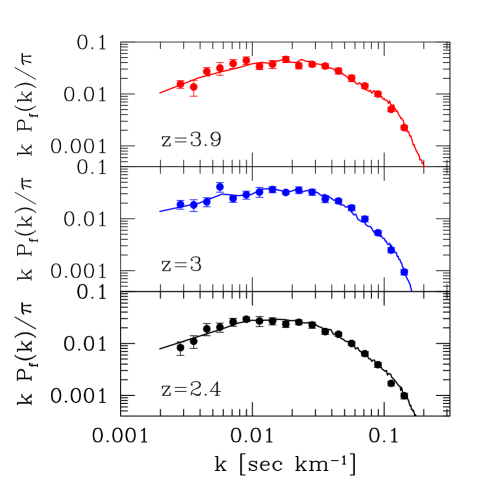
Figure 1.— Transmission power spectrum from from McDonald et al. (1999) together with our best fits.

In addition, we used the mean transmission as determined by McDonald et al. (1999) with their quoted errors (table 1).

$\bar{z}$	$\langle F\rangle$	$\sigma^{2}_{F}$
3.89	$0.475\pm 0.021$	$0.1293\pm 0.0030$
3.00	$0.684\pm 0.023$	$0.1174\pm 0.0056$
2.41	$0.818\pm 0.012$	$0.0789\pm 0.0068$

Table 1Mean ($\bar{F}=\langle F\rangle$) and variance ($\sigma^{2}_{F}$) of the transmission $F=e^{-\tau}$ as measured by McDonald et al. (1999) for several redshift bins.

3. Method

3.1. Model Predictions

The model predictions were done using the PM model for the forest (Croft et al. (1998); Meiksin & White (2000)). In this model PM simulations are run to compute dark matter densities and velocities. The gas density and temperature are calculated using simple scaling relations inspired by the results of full hydrodynamics simulations. Our objective is to constrain the parameters of these scaling relations.

We ran 7 PM simulations using $128^{3}$ particles with a box size $16h^{-1}{\rm Mpc}$ (corresponding to $3200{\rm km/sec}$ at redshift $z=3$) of the standard Cold Dark Matter (SCDM) model with different spectral indices $n=(0.4,0.7,0.9,1,1.1,1.3,$ $1.7)$ for the power spectrum of initial density perturbations. Having a non-vanishing cosmological constant will not significantly alter our results because $\Omega_{m}$ is close to $1$ at the relevant redshifts regardless of whether $\Lambda=0$ – the main determining factor is instead the power spectrum at certain scales, which we will constrain. We stored the density and velocity at expansion factors $a=\left(0.05,0.065,0.085,0.11,0.14,0.19,0.24,0.31,0.41\right)$. The expansion factors are used to span a range of power spectrum normalizations.

The baryon density is obtained by smoothing the dark matter density; the smoothing mimics the effect of pressure forces. Following Gnedin & Hui (1998) we adopt $\delta_{b}({\bf k})=W_{f}(k)\delta_{CDM}({\bf k})$ where $W(k)$ is a Fourier space smoothing, which we take to be $W_{f}(k)=\exp(-(k/k_{f})^{2})$. As discussed in Gnedin & Hui (1998), $k_{f}$ is proportional to the Jeans scale but the constant of proportionality depends on the details of the reionization history of the universe (see also Nusser 2000). For this reason, we treat $k_{f}$ as a free parameter. At redshift $z\sim 3$, the filtering is expected to be around $k_{f}\sim 35\ {\rm h\,Mpc^{-1}}$ (Gnedin & Hui 1998).

The optical depth for each gas element is related to the overdensity $\tau$ using a power law (Hui & Gnedin 1997a ),

$$\tau=a_{0}\Delta^{\beta}$$ (1)

where $\Delta=\rho/\bar{\rho}$ denotes the gas overdensity. The transmission is $e^{-\tau}$. The constant $a_{0}$ is fixed so that the generated spectra have a particular value of the mean transmission (which we will call $\bar{f}$). We make a grid of mean transmissions but use the observed measurements (in table 1) as a prior in our likelihood. Our grid of mean transmissions serves effectively as a grid of $a_{0}$’s.

For each grid point in the box a temperature is assigned to the gas using a simple power law equation of state for the gas,

$$T=T_{0}\Delta^{\alpha}.$$ (2)

We treat $T_{0}$ and $\alpha$ as free parameters. The power law index $\beta$ in equation (1) is related to $\alpha$, $\beta=2-0.7\alpha$. Smoothing due to thermal motions is included when the spectra are generated. The absorption produced by each fluid element is distributed in velocity space as $\exp(-(\Delta s/b)^{2})/b\sqrt{\pi}$, where $\Delta s$ is the velocity space separation and the $b$ parameter is given by $b=\sqrt{2kT/m_{p}}$ $\approx 13\ {\rm km}\ {\rm s}^{-1}$ for $T=10^{4}$ K.

Our parameter vector ${\bf p}=(a,n,k_{f},T_{0},\alpha,\bar{f})$ has 6 dimensions. We created a grid of model predictions for each choice of parameters in a grid,

• $a=(.05,.065,.085,.11,.14,.19,.24,.31,.41)$

• $n=(0.4,0.7,0.9,1,1.1,1.3,1.7)$

• $k_{f}=(5,10,20,30,40,45,50,55,60,70,80)$

• $T_{0}=\left(150,200,250,300,350,400,450,500,550,600,\right.$ $\left.700\right)$

• $\alpha=(0.0.0.1,0.2,0.3,0.4,0.5,0.6)$

• $\bar{f}=\left(.4,.45,.475,.5,.525,.55,.575,.6,.625,.65,.665,\right.$ $\left..684,.7,.725,.75,.78,.8,.82,.85,.9\right)$

where by convention the scale factor is $a=1/(1+z)$, $k_{f}$ is measured in ${\rm hMpc^{-1}}$ and $T_{0}$ in $({\rm km}{\rm s}^{-1})^{2}$. Thus we have a total of $9\times\ 7\times\ 11\times\ 11\times\ 7\times 20=1067220$ combinations of model parameters. For each point in our grid we extract 500 lines of sight randomly from the simulations, generate spectra and measure the power spectra of the forest. We measure the power spectra of the relative transmission fluctuations, $\delta F/\bar{F}$ where $F=\exp(-\tau)$.

3.2. Likelihood calculation

For each model in our grid, we compute the likelihood by comparing the power spectra computed form the simulations to the points in McDonald et al. (1999). In this paper, we will stick to a crude Gaussian approximation,

$$\L({\bf d};{\bf p})\propto\prod_{i}\exp\left[-{1\over 2}\left({d_{i}-P_{fi}({\bf p})\over\sigma_{i}}\right)^{2}\right],$$ (3)

where $i$ runs over the different data points $d_{i}$, the model prediction for that wavevector are $P_{fi}({\bf p})$ and $\sigma_{i}$ are the error bars on each point. By comparing different realizations we computed the statistical errors in our model predictions, which were approximately $5\%$. We added those in quadrature to the observational errors to compute $\sigma_{i}$. The addition of this extra source of variance makes very little difference because the observational errors are significantly larger. Most certainly systematic errors associated with our simplified model of the forest will dominate the error budget. We also used the last two points ($k\geq 0.1{\,\rm km^{-1}\,{\rm s}}$) as upper limits. To do so in practice we increased $\sigma$ for those points to $\sigma=0.3P_{f}$, roughly a factor of three increase on the quoted error bars and used it as a one sided error bar. For models that had more power than $P_{f}$ we computed $\chi^{2}$ with the increased error, for models with less power, we set the contribution to $\chi^{2}$ from that point to zero.

The data points reported in McDonald et al. (1999) are for the power spectrum of the transmission $\delta F$, and this is what we directly compare our predictions with (see, however, §5 for virtues of using power spectrum of $\delta F/\bar{F}$ instead). We furthermore add to the likelihood a term to account for the measurement of $\bar{F}$. We multiply the likelihood in 3 by $\exp(-(\bar{f}-\bar{F})^{2}/\sigma_{F}^{2})$ where $\bar{f}$ is the parameter in our grid and $\bar{F}$ is the observed value at the appropriate redshift. The error in the mean transmission is denoted $\sigma_{F}$.

The full likelihood function is $\L=e^{-\chi^{2}/2}$, where $\chi^{2}$ is simply the chi-squared goodness of fit of the model to the data. We have chosen to keep things this simple because we are in any case unable to eliminate a major source of inaccuracy: most probably there are correlations between the estimates of the power on different scales which are hard to estimate. We are using 18 bins for the power spectrum, thus estimating a covariance matrix requires estimating 153 numbers. Naive estimates of the covariance matrix based on a limited number of lines of sight are very noisy which translates into artificially low probabilities for some models, thus they cannot be used in this analysis. More theoretical work needs to be done in order to address this problem in a satisfactory manner. Perhaps one could look for guidance in simulations to build a simple parametrised model of the covariance matrix and then use the scatter between the lines of sight to fix those parameters. Moreover the window function needed to relate observed and theoretical power spectra are not available for this observation. We choose to use flat windows inside each bin but also tried Gaussian windows, which made only minor differences. There is ample room for improvement in this part of the calculation.

Once we have computed the likelihood for every model in our grid we marginalize along one direction at a time until we get one- or two-dimensional constraints on parameters. We use the method developed in Tegmark & Zaldarriaga (2000) for this purpose.

4. Results

In this section we report the constraints we have obtained. We first discuss our results on the equation of state of the IGM, then on the relation between baryons and dark matter and finally we summarize our constraints on the power spectrum of primordial fluctuations.

4.1. The temperature of the IGM

The shape of the power spectrum of the forest has a sharp cut-off around $k=0.02\ {\rm km^{-1}\ {\rm s}}$ which is due to the thermal broadening of the lines. Figure 2 shows a sequence of models with increasing IGM temperature. As the temperature increases the smoothing becomes more important and the power on small scales is reduced. At $k\sim 0.04\ {\rm km^{-1}\ sec}$ the power is down a factor of 2 from the extrapolation of the larger wavelengths. This corresponds to a temperature $T\sim 1/k\sim 2\times 10^{4}K$. Our likelihood analysis takes advantage of this dependence to find constraints on the temperature.

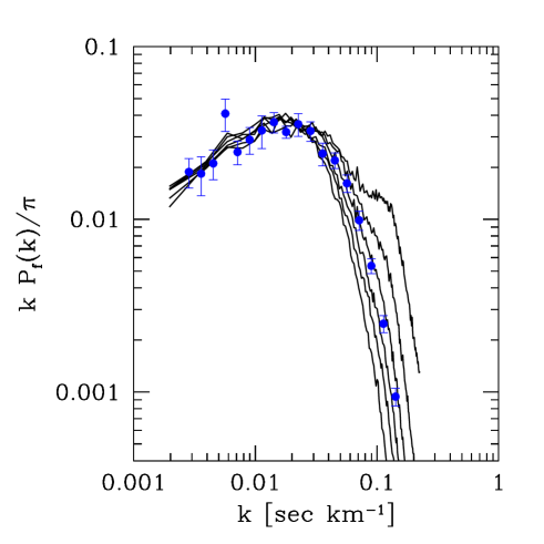
Figure 2.— Transmission power spectrum at $z=3$ for models with varying $T_{0}$ ($T_{0}=(150,250,\cdots,650)({\rm km}/{\rm s})^{2}$ increasing from top to bottom). All other parameters are left constant, ${\bf p}=(.24,.7,50,T_{0},.2,.7)$. The data points are from McDonald et al. (1999).

Figure 3 summarizes the constraints we obtained. It shows $95\%$ confidence regions in the $T_{0}-\alpha$ plane. Only $\alpha$’s between $0$ and $0.6$ are examined, because realistic $\alpha$ are expected to fall in this range (Hui & Gnedin 1997a ). We find a degeneracy in this plane, which is caused by the fact that our constraint is most tight for the temperature at a density different from the mean density. Under the assumption that the temperature density relation is a power law, the temperature at any given overdensity $\Delta_{*}$ can be calculated from $(T_{0},\alpha)$ as:

$$T_{*}=T_{0}\ \Delta_{*}^{\alpha}.$$ (4)

Our method to determine the temperature is most sensitive to $T_{*}$, so models with the same $T_{*}$ are all good fits to the data. This set of models correspond to lines in the $T_{0}-\alpha$ plane.

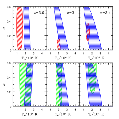
Figure 3.— Constraints in the $T-\alpha$ plane (95 % as described in the text). The top panel corresponds to the mean density while the bottom panel is for an overdensity $\Delta_{*}$. The ellipses with lines at $45^{o}$ angle on the top are the equivalent constraints from Schaye et al. (2000). and on the bottom from McDonald et al. (1999)

To investigate what $\Delta_{*}$ is, we run simulations in which the temperature-density relation has a step at a fixed overdensity $\Delta_{jump}$,

$$T = T_{0}\ ({\rm if}\ \Delta<\Delta_{jump})$$ (5)

$$= 2T_{0}\ ({\rm if}\ \Delta>\Delta_{jump})$$

with $T_{0}=1.2\ 10^{4}{\rm K}$. In figure 4 we show the change in the transmission power spectrum as we change the value of $\Delta_{jump}$ for a model that fits the observations at redshift $z=3$. For low values there is no change. When $\Delta_{jump}\sim 1$ changes become noticeable but once $\Delta_{jump}>1.8$ further increases in $\Delta_{jump}$ no longer change the power spectrum. At redshift $z=3$ the transmission power spectrum is therefore sensitive to $0.9<\Delta<1.8$. Given that our method is most sensitive to $\Delta$’s larger that one, the contours of equal likelihood are tilted in the $(T_{0},\alpha)$ plane in figure 3. On the other hand, because the method is intrinsically sensitive to a range of overdensities, it should be possible to extract information about $\alpha$ once the errors in the measured power decrease. The bottom panel of figure 3 shows our constraints at $\Delta_{*}=1.4$ constructed by reparametrizing our model grid using equation 4.

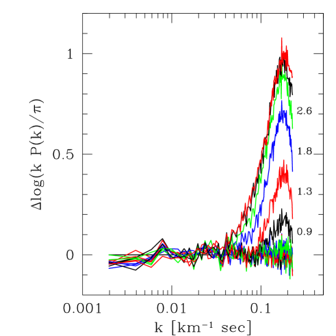
Figure 4.— Differences in the power spectrum of the flux of the forest at redshift $z=3$ for models with a step like temperature density relation as described in the test. Labels on the right indicate the value of $\Delta_{jump}$

A complementary method to determine the temperature was proposed in Schaye et al. (1999) and implemented in McDonald et al. (2000), Ricotti et al. (2000)and Schaye et al. (2000). The method is based on the observation that the width of the lines in the spectrum has several contributions, from thermal broadening, peculiar velocities and the intrinsic sizes of the structures (Hui and Rutledge (1999)). The minimum width of the lines is thus a measure of the thermal broadening. In the three papers cited above, the distribution of widths of lines was used to infer constraints on the temperature, two of which are shown as ellipses in our plot. We emphasize that those constraints were obtained fitting lines and determining a minimum width in their distribution. Our constraint did not require the fitting of lines. Although the analyses of Schaye et al. (1999) and McDonald et al. (2000) are based on the same underlying idea and very similar data sets, they differ in several technical details and agree neither in their conclusions nor in the size of their error bars.

Our results are in good agreement with those of McDonald et al. (2000) and we have comparable error bars. Our temperature is higher than that of Schaye et al. (2000). This could signal a bias in one of the methods, an underestimate of the errors or some unaccounted for physical effect. For example, to interpret the line fitting results one needs to know what gas density is responsible for the majority of the absorption. Simulations are usually used for this purpose and errors in this determination can lead to changes in the inferred temperatures. If the difference is not systematic, then a particularly interesting possibility is an inhomogeneous equation of state, which could be produced by a recent reionization of Helium II (see e.g. Madau 2000 for a review). In that case, the temperature measured from the cut-off in the line width distribution would tend to be lower because the method tends to use lines in places with a smaller mean temperature.

4.2. The relation between dark matter and baryons

The baryons experience pressure forces, so their distribution on small scales may not be the same as that of the dark matter. In our technique, we model this effect by smoothing the dark matter distribution to get the gas density using a 3D filter with a constant filtering scale across the box ($k_{f}$). In analytic models, $k_{f}$ depends on the temperature of the IGM and on its reionization history. The smoothing scale is one of the parameters in the grid so we marginalize over it when obtaining constraints on other parameters.

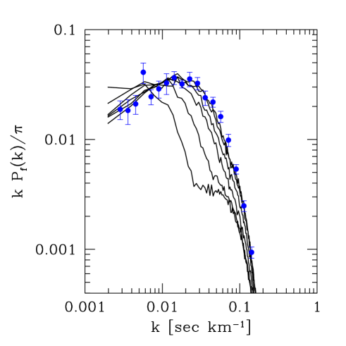
Figure 5.— Transmission power spectrum at $z=3$ for models with varying $k_{f}$ ($k_{f}=(5,10,20,30,40){\rm hMpc^{-1}}$ from bottom to top). All other parameters are left constant, ${\bf p}=(.24,.7,k_{f},400,.2,.7)$ . The data points are from McDonald et al. (1999).

Even though we have $k_{f}$ as a free parameter to marginalize over, we still get constraints on the temperature of the IGM. It is interesting to understand why that is the case, because both effects are a form of smoothing. The key is that the $k_{f}$ smoothing of the density field is done in 3D. After smoothing, a nonlinear transformation is applied to the density to obtain the flux. This transformation shifts power between scales, distorting the shape of the transmission power spectrum. Figure 5 illustrates the effect. For large smoothing scales (small $k_{f}$), the shape of the transmission power spectrum is totally wrong. Only when the smoothing by $k_{f}$ is subdominant to smoothing produced by thermal broadening are the fits acceptable. Note that some of our higher $k_{f}$’s probably approach the resolution limit of our simulations. We obtain lower limits on $k_{f}$, $k_{f}>10,30,25\ \ {\rm h\,Mpc^{-1}}$ for $z=2.4,3,3.9$ which can be compared with the Nyquist cut-off of the simulation $k_{Nyq}=50{\rm hMpc^{-1}}$. Thus some care is needed when interpreting our lower limits, as they may be somewhat sensitive to our resolution. In any case, the conclusion that the 3D smoothing should be subdominant compared with what is produced by the temperature should be robust against increase in numerical resolution.

4.3. The power spectrum of mass fluctuations

Finally we want to consider constraints on the power spectrum of mass fluctuations. Figure 6 shows our constraints in the amplitude/spectral index plane. The top panel shows directly the contours in our primary variables $(a,n)$, the expansion factor of our simulation and the primordial spectral index.

In the bottom panel of figure 6, we have changed our contours to the $(\Delta^{2},n_{eff})$ plane, where $\Delta$ is the amplitude and $n_{eff}$ is the spectral index of the linear power spectrum at $k=0.008\ {\rm km^{-1}\ sec}$. We did this to compare with the constraints from Croft et al. (1999) shown with a red ellipse. Although we agree in the range of allowed amplitudes, we disagree in the ability of the data to constrain the spectral index. The reason we cannot constrain the spectral index from the shape of the transmission power spectrum can be traced to our having $k_{f}$ as a free parameter. Figure 5 shows that changes in $k_{f}$ modify the low $k$ slope of the transmission power spectrum.

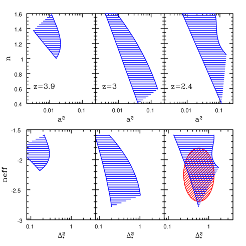
Figure 6.— The Constraints on amplitude and spectral index of the power spectrum of initial fluctuations. In the top we show constraints in our grid variables. On the bottom we have transformed this constraints to amplitude and spectral index of the initial power spectrum at $k=0.008\ {\rm km^{-1}\ sec}$ to compare with the constraints form Croft et al. (1999) shown with an ellipse (lines at $45^{o}$ angle).

In figure 7 we plot two models with very similar transmission power spectrum but with $n=0.4$ and $n=1.6$. The difference in slope, which should otherwise be noticeable at low $k$, is compensated by a change in $k_{f}$. This change in $k_{f}$ should produce changes in the power spectrum at high $k$, which is offset by a change in $T_{0}$. Thus the power spectrum data alone cannot accurately constrain the shape of the matter power spectrum unless other information is used to constrain $k_{f}$.

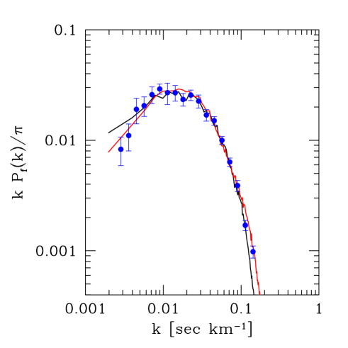
Figure 7.— Two models with very different spectral index that have similar flux power spectra together with the $z=2.4$ data. One model has ${\bf p}=(.41,.4,70,350,.3,.82)$ with $\chi^{2}=11$ and the other has ${\bf p}=(.14,1.6,20,250,.2,.82)$ with $\chi^{2}=10$.

5. Improvements for the future

The objective of this work was to show that detailed analysis of the transmission power spectrum can be used to extract useful information about the cosmological model and the properties of the IGM at high redshift. In order to make progress and extract more information from the data, there are several aspects of our work that could be improved in the future.

From an observational perspective, we need to improve the determination of the transmission power spectrum. Important ingredients will be to obtain a reliable covariance matrix for the different band powers and to determine the window functions that relate the observed power with the theoretical predictions. It would also be desirable to measure the power spectrum of $\delta F/\bar{F}$ after trend-removal rather than the power spectrum of $\delta F$ after continuum-fitting (Hui et al. 2000), to minimize systematic errors due to continuum placement.

From a theoretical perspective, one should study in more detail the relation between baryons and dark matter. Hydrodynamic simulations as well as the hydro-PM approximation (Gnedin & Hui (1998)) should be used to understand and quantify the possible biases introduced when extracting different parameters from PM simulations. Our method requires exploring a large number of models, so it will rely on dark matter only simulations (or the hydro-PM variant) for the foreseeable future.

A very interesting possibility is to try to determine if there are spatial fluctuations in the equation of state of the IGM. This will require measuring the transmission power spectrum and inferring a temperature for individual portions of spectra along different lines of sight and comparing results. A comparison will only be meaningful if one understands the expected distribution for these band-powers from simulations. It is important to know what one expects from cosmic variance alone and how different band powers are correlated in models with uniform equation of state.

Another direction which should be pursued is the combination of the power spectrum analysis with other information, in particular the probability distribution function (PDF) of the transmission. It will be interesting to know if the PDF can break some of the degeneracies we encountered. It is expected however that some degeneracies between parameters will remain (Theuns et al. 2000).

6. Conclusions

We have implemented a simple likelihood method to constrain the parameters of a Lyman $\alpha$ forest model from transmission power spectrum data. We used a 6 parameter grid and a marginalization method based on previous work for CMB data Tegmark & Zaldarriaga (2000). It is important that we fit for the 6 parameters simultaneously, as we find several parameter degeneracies that prevent us from extracting tighter constraints.

Perhaps our most interesting constraint is that on the equation of state of the gas. Our results are in good agreement with those of McDonald et al. (2000). We find a temperature that is somewhat higher than might have been expected and see little evidence for strong evolution of the temperature with redshift. Our determinations of the mean temperature and of temperature-density slope are highly degenerate.

As for the constraints on the mass power spectrum, we find amplitude constraints that are in agreement with those found by Croft et al. (1999). On the other hand, we are unable to place accurate constraints on the spectral index of the power spectrum, mainly due to an uncertainty in the relation between baryons and dark matter, parametrized by a smoothing scale $k_{f}$. This uncertainty is in part a consequence of our using dark matter only simulations to model the forest. Thus if one could construct a grid using hydrodynamic simulations, perhaps using the hydro-PM method of Gnedin & Hui (1998), some of this uncertainty could be removed. However, that part of the uncertainty in $k_{f}$ which is due to our ignorance of the reionization history will remain.

An important finding regarding smoothing is that the 3D smoothing parametrized by $k_{f}$ is less important than the 1D smoothing due to thermal broadening in determining the small scale transmission power spectrum. This is what allows us to determine the temperature of the IGM from the rapid fall-off in the small scale power. A $k_{f}$ small enough to affect the fall-off would also modify the shape of the transmission power spectrum sufficiently to make it an unacceptable match to observations.

Acknowledgements We would like to thank Joop Schaye for useful discussions. M.Z. is supported by the Hubble Fellowship HF-01116-01-98A from STScI, operated by AURA, Inc. under NASA contract NAS5-26555. L.H. is supported by NASA NAG5-7047 and the Taplin Fellowship at the IAS, and by an Outstanding Junior Investigator Award from the DOE. MT is supported by NASA grant NAG5-9194 and NSF grant AST00-71213 and the University of Pennsylvania Research Foundation.

References

- Bi et al. (1992) Bi H. G., Boerner G., Chu Y.,1992, A&A, 266, 1
- Bi & Davidsen (1997) Bi H. G., Davidsen A. F. 1997, ApJ, 479, 523
- Cen et al. (1994) Cen R., Miralda-Escude J., Ostriker J. P., Rauch M. 1994, ApJ, 437, L9
- Croft et al. (1997) Croft R. A. C., Weinberg D. H., Hernquist L., Katz N. 1997, ApJ, 488, 532
- Croft et al. (1998) Croft R. A. C., Weinberg D. H., Katz N., Hernquist L. 1998, ApJ, 495, 44
- Croft et al. (1999) Croft R. A. C., Weinberg D. H., Pettini M., Hernquist L., Katz N. 1999, ApJ, 520, 1
- Gaztanaga & Croft et al. (1999) Gaztanaga E., Croft R. A. C. 1999 MNRAS309, 885
- Gnedin & Hui (1996) Gnedin N. Y., Hui L., 1996, ApJ, 472, 73
- Gnedin & Hui (1998) Gnedin N. Y., Hui L., 1998, MNRAS, 296, 44
- Hernquist et al. (1995) Hernquist L., Katz N., Weinberg D. H., Miralda-Escude J. 1995, ApJ, 457, L5
- Hui (1999) Hui L. 1999, ApJ, 516, 519
- Hui et al. (2000) Hui L., Burles S., Seljak U., Rutledge R. E., Magnier E., Tytler D. 2000, submitted to ApJ, astro-ph 0005049
- (13) Hui L., Gnedin N. Y. 1997a, MNRAS, 292, 27
- (14) Hui L., Gnedin N. Y., Zhang Y. 1997b, ApJ, 486, 599
- Hui and Rutledge (1999) Hui L., Rutledge R. E. 1999, ApJ, 517, 541
- Madau (2000) Madau P. 2000, Phil. Trans. R. Soc. London A, 358
- McDonald & Miralda-Escude (1999) McDonald, P. & Miralda-Escude, J. 1999, ApJ, 518, 24.
- McDonald et al. (1999) McDonald P., Miralda-Escude J., Rauch M., Sargent W. L. W., Barlow T. a. , Cen R., Ostriker J. P., preprint astro-ph/9911196
- McDonald et al. (2000) McDonald P., Miralda-Escude J., Rauch M., Sargent W. L. W., Barlow T. a. , Cen R., Ostriker J. P., preprint astro-ph/0005553
- Meiksin & White (2000) Meiksin A., White M. 2000, submitted to MNRAS, astro-ph 0008214
- Miralda-Escude et al. (1996) Miralda-Escude J., Cen R., Ostriker J. P., Rauch M. 1996, ApJ, 471, 582
- Muecket et al. (1996) Muecket J. P., Petitjean P., Kates R. E., Riediger R. 1996, A&A, 308, 17
- Narayanan et al. (2000) Narayanan V. K., Spergel D. N., Dave R., Ma C. P. 2000, preprint astro-ph/0001247
- Nusser (2000) Nusser A. 2000, MNRAS, 317, 902
- Nusser & Haehnelt (2000) Nusser A., Haehnelt M. 2000, MNRAS, 313, 364
- Rauch et al. (1997) Rauch, M., Miralda-Escude, J., Sargent, W. L. W., Barlow, T. A., Weinberg, D. H., Hernquist, L., Katz, N., Cen, R. & Ostriker, J. P. 1997, ApJ, 489, 7
- Reisenegger & Miralda-Escude (1995) Reisenegger A., Miralda-Escude J. 1995, ApJ, 449, 476
- Ricotti et al. (2000) Ricotti M., Gnedin N. Y., Shull M. 2000, ApJ, 534, 41
- Schaye et al. (1999) Schaye J., Theuns T., Leonard A., Efstathiou G. 1999, MNRAS, 310, 57
- Schaye et al. (1999) Schaye J., Theuns T., Rauch M., Efstathiou G., Sargent W. 2000, MNRAS, 318, 817
- Theuns et al. (1998) Theuns T., Leonard A., Efstathiou G., Pearce F. R., Thomas P. A. 1998, MNRAS, 301, 478
- Theuns et al. (2000) Theuns T., Schaye J., Haehnelt M., MNRAS, 315, 600
- Tegmark & Zaldarriaga (2000) Tegmark M., Zaldarriaga M., astro-ph/0002091
- Wadsley & Bond (1996) Wadsley J. W., Bond J. R. 1996, Proceeding of the 12th Kingston Conference, eds. Clarke D., West M., PASP, astro-ph/9612148
- White & Croft (2000) White M., Croft R. A. C. 2000, preprint astro-ph/0001247
- Zhang et al. (1995) Zhang Y., Anninos P., Norman M. L. 1995, ApJ, 453, L57