Abstract

Dynamical studies of MHD turbulence on the one hand, and arguments based upon magnetic helicity on the other, have yielded seemingly contradictory estimates for the $\alpha$ parameter in turbulent dynamo theory. Here we show, with direct numerical simulation of three-dimensional magnetohydrodynamic turbulence with a mean magnetic field, $\overline{{\bf B}}$, that the constraint on the dynamo $\alpha$-effect set by the magnetic helicity is time-dependent. A time-scale $t_{c}$ is introduced such that for $t<t_{c}$, the $\alpha$-coefficient calculated from the simulation is close to the result of Pouquet et al. and Field et al. , $-\frac{\tau_{cor}}{3}(\langle{\bf v}\cdot\nabla\times{\bf v}\rangle-\langle{\bf b}\cdot\nabla\times{\bf b}\rangle)$; for $t>t_{c}$, the classical result of the $\alpha$-coefficient given by the Mean-Field Electrodynamics is reduced by a factor of $1/\left({R_{m}|\overline{{\bf B}}|^{2}/v_{rms}^{2}}\right)$, as argued by Gruzinov & Diamond, Seehafer and Cattaneo & Hughes. Here, $R_{m}$ is the magnetic Reynolds number, $v_{rms}$ the rms velocity of the turbulence, $\tau_{cor}$ the correlation time of the turbulence, and $\overline{B}$ is in velocity unit. The applicability of and connection between different models of dynamo theory are also discussed.

1 Introduction

The generation and amplification of magnetic field in many astrophysical systems are often attributed to the turbulent dynamo effect. Since the seminal papers by Parker (1955) and Steenbeck, Krause & Rädler (1966), a whole body of theory, namely, Mean Field Electrodynamics (MFE) has been developed to explain the dynamics of magnetic field generation by helical turbulence in a conducting fluid (Moffatt 1978, or Krause & Rädler 1980). In such a fluid, the velocity field, ${\bf v}$, stretches the magnetic field, ${\bf b}$, in such a way that the correlation of ${\bf v}$ and ${\bf b}$ results in an electromotive force, $\langle{\bf v}\times{\bf b}\rangle$ that amplifies the mean (large-scale) magnetic field, $\overline{{\bf B}}$, through the relation

$$\langle{\bf v}\times{\bf b}\rangle=\alpha\overline{{\bf B}}.$$ (1)

Here, the coefficient $\alpha$ represents the so-called $\alpha$-effect (Moffatt 1978); it is calculated in MFE as $\alpha_{MFE}\sim-\frac{\tau_{cor}}{3}\langle{\bf v}\cdot\nabla\times{\bf v}\rangle$, where $\tau_{cor}$ is the correlation time of the turbulence. MFE is a kinematic theory, in that the velocity field is prescribed and no back reaction of the magnetic field on the velocity field is considered. Therefore, its applicability to circumstances where the velocity field is affected by the growing magnetic field is questionable. Several authors have extended MFE to include the quenching of the $\alpha$-effect due to the back reaction of the magnetic field. By numerically solving the spectral MHD equations using a closure method known as the EDQNM (Eddy-Damped Quasi-Normal Markovian) approximation, Pouquet, Frisch & Léorat (1976, hereafter PFL) find that $\alpha=\int_{k}\alpha_{k}dk$, where $\alpha_{k}$ is determined by, in Fourier space, the difference between the spectra of the kinetic helicity correlation function, $\langle{\bf v}\cdot\nabla\times{\bf v}\rangle$, and the current helicity correlation function, $\langle{\bf b}\cdot\nabla\times{\bf b}\rangle$. A similar result was found by Field, Blackman & Chou (1999, hereafter FBC), who consider the back reaction of magnetic field by treating ${\bf v}$ and ${\bf b}$ on an equal footing, and give a model in which the $\alpha$-coefficient (for later purposes, we call it $\alpha_{1}$) can be expressed as

$$\alpha_{1}=-\frac{\tau_{cor}}{3}\left(\langle{\bf v}\cdot\nabla\times{\bf v}\rangle-\langle{\bf b}\cdot\nabla\times{\bf b}\rangle\right)$$ (2)

for relatively small values of $\left({\overline{B}}/{v_{rms}}\right)^{2}$.

However, the nonlinear nature of the problem introduces so much difficulty that the effect of the back reaction is still under debate. One of the objections to the application of $\alpha_{1}$ to the galactic dynamo has its root in the problem of large magnetic Reynolds number and small-scale fields. Vainshtein & Cattaneo (1992, see also Cattaneo & Vainshtein 1991) argue that for systems with large $R_{m}$, $\alpha$ is reduced by a factor of $R_{m}$ from its kinematic value, i.e.,

$$\alpha\propto\frac{1}{R_{m}},$$ (3)

as the small-scale magnetic field grows quickly to turn off the generation of magnetic flux at large scales. These authors applied the conservation of the square vector potential of 2D ideal MHD. The conservation of magnetic helicity of 3D MHD in steady state was later studied by Seehafer (1994, 1995) who provided another model of the dynamo $\alpha$-effect in which the $\alpha$-coefficient (for later purposes, we call it $\alpha_{2}$) is given by

$$\alpha_{2}=-\frac{\lambda\langle{\bf b}\cdot\nabla\times{\bf b}\rangle}{{\overline{B}}^{2}}.$$ (4)

Because $R_{m}=Lv_{rms}/\lambda$, $\alpha_{2}\propto 1/R_{m}$ also. Because $R_{m}\gg 1$ in astrophysical systems such as the Galaxy, both relation (3) and relation (4) suggest strong suppression of the dynamo $\alpha$-effect.

Another model of the dynamo $\alpha$-effect was introduced by Gruzinov & Diamond (1994, 1995, 1996) by studying how the conservation of magnetic helicity affects the result like relation (2). They realized that because Ohmic dissipation of the current helicity $\langle{\bf b}\cdot\nabla\times{\bf b}\rangle$ in (2) changes the magnetic helicity, the dynamics of the latter will affect $\alpha_{1}$, which should be modified to (for later purposes, we call it $\alpha_{3}$)

$$\alpha_{3}=\frac{\alpha_{MFE}}{1+R_{m}({\overline{B}}/v_{rms})^{2}}.$$ (5)

Since $R_{m}$ is usually very large in astrophysics, this again implies that $\alpha$, in steady state, is far smaller than its classical value, so that it is too small to be important for the generation of large scale magnetic fields. Note that in the limit of $R_{m}\gg 1$ and $v_{rms}\sim b_{rms}$, $\alpha_{3}$ is reduced to $\alpha_{2}$.

$\alpha_{2}$ and $\alpha_{3}$ are different from $\alpha_{1}$ in the following two aspects: first, $\alpha_{1}$ does not explicitly show strong suppression of the $\alpha$-effect for large $R_{m}$; second, neither of the dynamical studies of PFL and FBC, which give $\alpha_{1}$, explicitly considered the conservation of magnetic helicity that led to $\alpha_{2}$ and $\alpha_{3}$. Under what conditions the magnetic helicity constraint, which is essential in the models of $\alpha_{2}$ and $\alpha_{3}$, enters the derivation of $\alpha_{1}$ is still an open question. In other such words, if such magnetic helicity constraint can be relaxed in systems of large $R_{m}$, which of these three models remains valid? To provide insight into this problem, in the following we study the dynamics of magnetic helicity using the magnetic helicity conservation equations, and the time dependence of $\alpha$ using a numerical simulation of MHD turbulence. We find that both the magnetic helicity development and the $\alpha$-coefficient are time dependent. We find that the classical MFE result is valid up to a critical time that we calculate, and the magnetic helicity constrained result is valid thereafter. Which value to apply therefore depends on the circumstances.

This paper is presented in the following structure: in Section 2 we provide a model for the time-dependence of the magnetic helicity development, and introduce a critical time, $t_{c}$, to separate the two important stages of the magnetic helicity evolution; in Section 3.1 we present our numerical model that is used to study the time-dependence of the dynamo $\alpha$-effect; the numerical results are given in Section 3.2; in Section 4 we discuss the implications of our analytic model and the numerical results, which are applied to the Galactic dynamo; conclusions are given in Section 5.

2 The Time Dependence of Magnetic Helicity Dynamics

We start from studying the dynamics of the magnetic helicity and its constraint on the dynamo $\alpha$-effect. For a 3D incompressible MHD system, we separate the vector potential ${\bf A}$ into a large-scale part $\overline{{\bf A}}$ and a small-scale part ${\bf a}$. Similarly, we write the magnetic field as ${\bf B}=\overline{{\bf B}}+{\bf b}$ and the velocity field as ${\bf V}=\overline{{\bf V}}+{\bf v}$. By un-curling the induction equation for ${\bf B}$,

$$\frac{\partial{\bf B}}{\partial t}=\nabla\times\left({\bf V}\times{\bf B}\right)+\lambda\nabla^{2}{\bf B},$$ (6)

we have the equation for ${\bf A}$,

$$\frac{\partial{\bf A}}{\partial t}={\bf V}\times{\bf B}+\lambda\nabla^{2}{\bf A}-\nabla\psi.$$ (7)

Here $\lambda$ is the magnetic diffusivity and $\psi$ is the scalar potential. Dotting (6) with ${\bf a}$ and (7) with ${\bf b}$ and summing the resulting equations together, we have the equation for the ensemble average of the small-scale magnetic helicity

$$\frac{\partial}{\partial t}\langle{\bf a}\cdot{\bf b}\rangle = -2\lambda\langle{\bf b}\cdot\nabla\times{\bf b}\rangle-2\langle{\bf v}\times{\bf b}\rangle\cdot\overline{{\bf B}}$$ (8)

$$+ \langle\nabla\cdot\left(-{\bf b}\psi^{\prime}-{\bf a}\times({\bf v}\times{\bf b}+\overline{{\bf V}}\times{\bf b}+{\bf v}\times\overline{{\bf B}})\right)\rangle,$$

where $\psi^{\prime}$ is the fluctuating component of the scalar potential. The third term in (8) comes from the ${\bf v}\times\overline{{\bf B}}$ term in both (6) and (7), which represents the interaction between the small-scale velocity field ${\bf v}$ and the large-scale magnetic field $\overline{{\bf B}}$. The physics of this term can be explained as follows. The line stretching, twisting and folding of $\overline{{\bf B}}$ will produce ${\bf b}$ and ${\bf a}$, therefore affect the generation and diffusion of $\langle{\bf a}\cdot{\bf b}\rangle$ within a volume $V$. The divergence term shows that flux of magnetic helicity of certain sign can escape from the system through open boundaries (Blackman & Field, 2000). The equation for the large-scale magnetic helicity, $\overline{{\bf A}}\cdot\overline{{\bf B}}$, can be also derived. The equations for $\overline{{\bf B}}$ and $\overline{{\bf A}}$ are

$$\frac{\partial\overline{{\bf B}}}{\partial t}=\nabla\times\left(\overline{{\bf V}}\times\overline{{\bf B}}\right)+\nabla\times\langle{\bf v}\times{\bf b}\rangle+\lambda\nabla^{2}\overline{{\bf B}},$$ (9)

$$\frac{\partial\overline{{\bf A}}}{\partial t}=\overline{{\bf V}}\times\overline{{\bf B}}+\langle{\bf v}\times{\bf b}\rangle+\lambda\nabla^{2}\overline{{\bf A}}-\nabla{\overline{\psi}}.$$ (10)

Following similar procedures that led us to get (8), we have

$$\frac{\partial}{\partial t}(\overline{{\bf A}}\cdot\overline{{\bf B}}) = -2\lambda\overline{{\bf B}}\cdot\nabla\times\overline{{\bf B}}+2\langle{\bf v}\times{\bf b}\rangle\cdot\overline{{\bf B}}$$ (11)

$$+ \langle\nabla\cdot\left(-\overline{{\bf B}}{\overline{\psi}}-\overline{{\bf A}}\times(\overline{{\bf V}}\times\overline{{\bf B}}+\langle{\bf v}\times{\bf b}\rangle)\right)\rangle.$$

Note that the third term in (11) has the opposite sign of the third term in (8), showing that the electromotive force $\langle{\bf v}\times{\bf b}\rangle$ generates $\overline{{\bf A}}\cdot\overline{{\bf B}}$ of the opposite sign of $\langle{\bf a}\cdot{\bf b}\rangle$. If we define the following two flux terms

$${\bf f}=\langle{\bf b}\psi^{\prime}+{\bf a}\times({\bf v}\times{\bf b}+\overline{{\bf V}}\times{\bf b}+{\bf v}\times\overline{{\bf B}})\rangle,$$ (12)

$${\bf F}=\langle\overline{{\bf B}}{\overline{\psi}}+\overline{{\bf A}}\times(\overline{{\bf V}}\times\overline{{\bf B}}+\langle{\bf v}\times{\bf b}\rangle)\rangle,$$ (13)

with (12) and (13), we may re-write (8) and (11) in the limit of $\lambda\rightarrow 0$ in the form

$$D_{t}\langle{\bf a}\cdot{\bf b}\rangle\equiv\frac{\partial}{\partial t}\langle{\bf a}\cdot{\bf b}\rangle+\nabla\cdot{\bf f}=-2{\cal E}\cdot\overline{{\bf B}},$$ (14)

$$D_{t}(\overline{{\bf A}}\cdot\overline{{\bf B}})\equiv\frac{\partial}{\partial t}\overline{{\bf A}}\cdot\overline{{\bf B}}+\nabla\cdot{\bf F}=2{\cal E}\cdot\overline{{\bf B}},$$ (15)

where ${\cal E}=\langle{\bf v}\times{\bf b}\rangle$ is the electromotive force. The conservation of total magnetic helicity, $H_{m}=\langle{\bf a}\cdot{\bf b}\rangle+\overline{{\bf A}}\cdot\overline{{\bf B}}$, immediately follows from the above two equations and reads

$${\cal D}_{t}H_{m}\equiv D_{t}\langle{\bf a}\cdot{\bf b}\rangle+D_{t}(\overline{{\bf A}}\cdot\overline{{\bf B}})=0,$$ (16)

which holds for ideal MHD.

Seehafer (1994, 1995) related the dynamics of small-scale magnetic helicity, i.e., equation (8), to the quenching of the dynamo $\alpha$-effect. By assuming stationarity of the MHD turbulence in a closed system, he argued that $\partial_{t}\langle{\bf a}\cdot{\bf b}\rangle=0$ and $\nabla\cdot{\bf f}=\nabla\cdot{\bf F}=0$; therefore, by neglecting the time-dependent term and the boundary term in equation (8) and applying relation (1), he obtained relation (4) for $\alpha_{2}$. The same assumptions about the stationarity and the closedness of the system were made by Gruzinov & Diamond (1994, 1995, 1996), where they provide a modified $\alpha$-coefficient in the form of $\alpha_{3}$. $\alpha_{3}$ can be regarded as an interpolation between the MFE result $\alpha_{MFE}$ and the quenching result $\alpha=\frac{\alpha_{MFE}}{R_{m}({\overline{B}}/v_{rms})^{2}}$ (see also Cattaneo & Vainshtein, 1991 and Vainshtein & Cattaneo, 1992), thus it is supposed to be valid for both large and small $R_{m}$. The numerical simulation by Cattaneo & Hughes (1996) with a particular $R_{m}=100$ and different values of $\overline{{\bf B}}$ supports this result.

$\alpha_{2}$ and $\alpha_{3}$ are different from $\alpha_{1}$ in that both of these two models show strong suppression of $\alpha$ for large $R_{m}$. The large magnetic Reynolds number $R_{m}$ in real astrophysical systems constrains the dynamo $\alpha$-effect to such a degree that, according to these two models, $\alpha$ would be too small to be important. However, from the above derivation of both $\alpha_{2}$ and $\alpha_{3}$, one can see that three conditions must be met in order for such constraint to be effective in real astrophysical systems:

• a large magnetic Reynolds number,

• the system is in stationary state, and

• the system is closed, i.e, no net flux of magnetic helicity flowing through the system.

Because the numerical simulation of Cattaneo & Hughes (1996) satisfies all these conditions, it is interesting that their numerical results confirm $\alpha_{3}$ in relation (5).

For real astrophysical systems, these three conditions may not be satisfied simultaneously. For example, Blackman & Field (2000) have argued that most astrophysical objects are open systems, and magnetic helicity can flow through the boundaries. For systems where $\overline{{\bf B}}$ cannot be assumed constant, Bhattacharjee & Yuan (1995) suggested that $\alpha\rightarrow\frac{1}{{\overline{B}}^{2}}\nabla\cdot\left(\kappa^{2}\nabla\frac{{\overline{\bf J}}\cdot\overline{{\bf B}}}{{\overline{B}}^{2}}\right)$ for $R_{m}\rightarrow\infty$, where ${\overline{\bf J}}=\nabla\times\overline{{\bf B}}$ and $\kappa^{2}$ is a positive functional of the statistical properties of the MHD turbulence.

Another assumption made in deriving $\alpha_{2}$ and $\alpha_{3}$, the stationarity of the MHD turbulence, may also not be valid when the $\alpha$-coefficient in relations (4) or (5) is applied to real astrophysical systems. One scenario that we can imagine is that when impulsive, transient phenomena such as solar flares or supernova explosions happen, steady astrophysical systems will be disturbed. This means that, to correctly understand the relation between the dynamics of magnetic helicity and the dynamo $\alpha$-effect and its application to real astrophysical systems, one should study not only the stationary state where the magnetic helicity has been built up in the system, but also the non-stationary state when there is net magnetic helicity being built up in or thrown away from the system. During such non-stationary state of the magnetic helicity development, the velocity field has the freedom to stay independent from the growing magnetic field, and if so, the derivation of $\alpha_{2}$ from just the induction equation may not give a complete picture for the dynamo $\alpha$-effect in real astrophysical systems (Kulsrud 1999). On the other hand, both PFL and FBC, who give $\alpha_{1}$ in dynamical studies, incorporate not only the momentum equation but also the induction equation into their models. Because $\alpha_{3}$ can be derived by relating the $\langle{\bf b}\cdot\nabla\times{\bf b}\rangle$ terms in relations (4) and (2), it is expected that $\alpha_{3}$ should include not only the dynamical considerations of PFL and FBC but also the magnetic helicity constraint of Seehafer. However, in order to derive $\alpha_{3}$ in this way, one has to assume that $\alpha_{1}$ is equivalent to $\alpha_{2}$ in order to get $\alpha_{3}$ in the form of relation (5). This means that the assumptions of closedness, stationarity and large $R_{m}$ must be satisfied in the model of $\alpha_{3}$.

If the stationarity assumption is removed, the magnetic helicity constraint shown in the models of $\alpha_{2}$ and $\alpha_{3}$ can then be relaxed, even though in these models the magnetic Reynolds number is large and the system is closed. And if the magnetic helicity constraint is relaxed, the model of $\alpha_{1}$ may give a complete picture of the dynamo $\alpha$-effect. If the relaxation of the magnetic helicity constraint lasts for a limited period of time, the model of $\alpha_{1}$ must be extended so that the magnetic helicity conservation is taken into account by introducing $\alpha_{2}$ and $\alpha_{3}$. Note that $\alpha_{2}\sim\alpha_{3}$ for large $R_{m}$, and we are only interested in large $R_{m}$ (or small $\lambda$, as in astrophysics) case.

To test our hypothesis of the non-stationary state of a 3D MHD system, we consider a closed system and neglect the boundary effects due to $\nabla\cdot{\bf f}$ and $\nabla\cdot{\bf F}$. The resulting equations for the small and large scale magnetic helicity can be written as

$$\frac{\partial}{\partial t}\langle{\bf a}\cdot{\bf b}\rangle=-2\lambda\langle{\bf b}\cdot\nabla\times{\bf b}\rangle-2\alpha{\overline{B}}^{2},$$ (17)

and

$$\frac{\partial}{\partial t}(\overline{{\bf A}}\cdot\overline{{\bf B}})=-2\lambda\overline{{\bf B}}\cdot\nabla\times\overline{{\bf B}}+2\alpha{\overline{B}}^{2},$$ (18)

where relation (1) is used. The interpretation of equations (17) and (18) is that: the production of positive/negative large-scale magnetic helicity, $\overline{{\bf A}}\cdot\overline{{\bf B}}$, by the dynamo $\alpha$-effect is due to the production of negative/positive small-scale magnetic helicity, $\langle{\bf a}\cdot{\bf b}\rangle$ and to dissipation, $\lambda\langle\overline{{\bf B}}\cdot\nabla\times\overline{{\bf B}}\rangle$. For systems with $\lambda\rightarrow 0$, the total magnetic helicity, $\overline{{\bf A}}\cdot\overline{{\bf B}}+\langle{\bf a}\cdot{\bf b}\rangle$, is conserved, and dynamo $\alpha$-effect can be understood as a pumping effect that transfers small-scale magnetic helicity to large scales without generating any total magnetic helicity in the (closed) system. To illustrate such a pumping effect, consider the case that at certain time the small-scale magnetic helicity is zero, $\langle{\bf a}\cdot{\bf b}\rangle=0$. A dynamo $\alpha$-effect with positive $\alpha$ coefficient will pump positive magnetic helicity from small scales to large scales, and leave negative magnetic helicity at small scales, so that after some critical time $t_{c}$, $\langle{\bf a}\cdot{\bf b}\rangle<0$, $\overline{{\bf A}}\cdot\overline{{\bf B}}>0$, and $\langle{\bf a}\cdot{\bf b}\rangle+\overline{{\bf A}}\cdot\overline{{\bf B}}=0$.

To quantify these effects, consider the case in (17) that $\lambda$ is very small so that the diffusion term can be neglected. If at $t=0$, $\langle{\bf a}\cdot{\bf b}\rangle=0$, the integral of the resulting equation gives

$$\langle{\bf a}\cdot{\bf b}\rangle(t)=-2{\overline{B}}^{2}\int_{0}^{t}\alpha(\tau)d\tau.$$ (19)

For small times, when the constraint of magnetic helicity on the dynamo effect is not yet effective, we assume that

$$\alpha(t)=\alpha_{1},$$ (20)

the dynamical value calculated by the model of $\alpha_{1}$, so

$$\langle{\bf a}\cdot{\bf b}\rangle(t)\cong-2{\overline{B}}^{2}\alpha_{1}t.$$ (21)

This should be valid for small values of $t$. However, as $t$ increases, $\langle{\bf a}\cdot{\bf b}\rangle(t)$ approaches the maximum that can be associated with the given small-scale magnetic energy. It can be shown from the realizability condition (Moffatt 1978) that

$$|\langle{\bf a}\cdot{\bf b}\rangle(t)|\leq 2Lb_{rms}^{2},$$ (22)

where $L$ is the outer scale of the turbulence, and $b_{rms}$ is the rms small-scale field strength. In light of this, (20) is valid only up to a critical time $t_{c}$ given by

$$t_{c}\cong\frac{Lb_{rms}^{2}}{\alpha_{1}{\overline{B}}^{2}}.$$ (23)

Since $\alpha_{1}\sim{\cal O}(v_{rms})$, where $v_{rms}$ is the rms velocity, and $L/v_{rms}=t_{eddy}$, the eddy turnover time,

$$t_{c}\cong t_{eddy}\left(\frac{b_{rms}}{\overline{B}}\right)^{2}.$$ (24)

A more realistic estimate of $t_{c}$ should include a correction factor, which modifies the above formula to $t_{c}\cong Ct_{eddy}\left(\frac{b_{rms}}{\overline{B}}\right)^{2}$. The correction factor $C$ depends on the ratio $v_{rms}/\alpha_{1}$ and the ratio $|\langle{\bf a}\cdot{\bf b}\rangle|/2Lb_{rms}^{2}$. $C$ can be estimated from numerical simulation results, as we will do in the next section.

When $t>t_{c}$, because there is no further small-scale magnetic helicity to draw on, $\partial_{t}\langle{\bf a}\cdot{\bf b}\rangle\rightarrow 0$, and from (17) we have

$$\alpha{\overline{B}}^{2}=-\lambda\langle{\bf b}\cdot\nabla\times{\bf b}\rangle,$$ (25)

which implies that $\alpha$ no longer equals $\alpha_{1}$, but rather is determined by the fact that the only available source for the large-scale magnetic helicity being pumped by $\alpha$ is that which is being dissipated at small scales with appropriate sign. That is, $\alpha$ equals $\alpha_{2}$, hence is suppressed by the large $R_{m}$ (or small $\lambda$) for the stage $t>t_{c}$. To estimate the value of the suppressed $\alpha$, $\alpha_{sp}$, we replace the current helicity of the small-scale magnetic field, $\langle{\bf b}\cdot\nabla\times{\bf b}\rangle$, with the value corresponding to a maximally helical small-scale field (which we assumed to result from (20) at $t=t_{c}$), which is

$$|\langle{\bf b}\cdot\nabla\times{\bf b}\rangle|\cong L^{-1}b_{rms}^{2}.$$ (26)

Hence

$$|\alpha_{sp}|\sim\frac{\lambda}{L}\left(\frac{b_{rms}}{\overline{B}}\right)^{2}.$$ (27)

Since $|\alpha_{1}|\sim v_{rms}$, and $R_{m}=Lv_{rms}/\lambda$, this can be written as

$$|\alpha_{sp}|\sim\alpha_{1}\frac{1}{R_{m}}\left(\frac{b_{rms}}{\overline{B}}\right)^{2}.$$ (28)

This formula is consistent with $\alpha_{3}$ when $R_{m}$ is large, and is identical to $\alpha_{2}$, the model by Seehafer (1994, 1995). However, notice that unlike previous derivations, ours depends critically on time; so

$$\frac{\alpha}{\alpha_{1}}=\left\{\begin{array}[]{ll}1&\mbox{$t<t_{c}=t_{eddy}\left(\frac{b_{rms}}{\overline{B}}\right)^{2}$,}\\ \frac{1}{R_{m}}\left(\frac{b_{rms}}{\overline{B}}\right)^{2}&\mbox{$t>t_{c}$.}\end{array}\right.$$ (29)

Note that neither $\alpha_{2}$ nor $\alpha_{3}$ appears in relation (29) because they should be valid only for $t>t_{c}$, when the magnetic helicity constraint takes effect.

In the above discussion, we made the following assumptions that require further justification: (1) the system has an amount of small-scale magnetic helicity that can be estimated as $Lb_{rms}^{2}$, where $L$ is the scale where the magnetic helicity is concentrated; (2) current helicity can be estimated as $b_{rms}^{2}/L$; (3) $v_{rms}^{2}\sim b_{rms}^{2}$. To test these assumptions and calculate $t_{c}$ as a function of $t_{eddy}b_{rms}^{2}/{\overline{B}}^{2}$, we apply direct numerical simulation to a 3D incompressible MHD system with periodic boundary conditions. The numerical model and simulation results are presented in next section.

3 Numerical Model and Simulation Results

3.1 Numerical Model

Under an external force $\cal F$, the undimensionalized incompressible MHD equations can be written as (with Einstein summation convention)

$$\left(\partial_{t}-\nu\nabla^{2}\right)v_{i}=\partial_{j}\left(-p\delta_{ij}-v_{i}v_{j}+b_{i}b_{j}\right)+{\cal F}_{i},$$ (30)

$$\left(\partial_{t}-\lambda\nabla^{2}\right)b_{i}=\partial_{j}\left(v_{i}b_{j}-b_{i}v_{j}\right),$$ (31)

$$\partial_{i}v_{i}=\partial_{j}b_{j}=0,$$ (32)

where $\nu$ and $\lambda$ are the molecular viscosity and magnetic diffusivity, respectively. Note that we have written $b$ in units of $\sqrt{4\pi\rho}$ after dividing both sides of the Navier-Stokes equation and the induction equation by density $\rho$. If we use a hat, $\wedge$, to denote discrete Fourier transform, and $\otimes$ to denote convolution, the above equations in Fourier space are

$$\left(\partial_{t}+\nu k^{2}\right){\hat{v}}_{j}=P_{jl}\left[\mbox{i}k_{m}\left(-{\hat{v}}_{l}\otimes{\hat{v}}_{m}+{\hat{b}}_{l}\otimes{\hat{b}}_{m}\right)+{\hat{\cal F}}_{l}\right],$$ (33)

$$\left(\partial_{t}+\lambda k^{2}\right){\hat{b}}_{j}=P_{jl}\left[\mbox{i}k_{m}\left({\hat{v}}_{l}\otimes{\hat{b}}_{m}-{\hat{v}}_{m}\otimes{\hat{b}}_{l}\right)\right],$$ (34)

$$k_{m}{\hat{v}}_{m}=k_{j}{\hat{b}}_{j}=0.$$ (35)

Here $\bf P$ is the projection operator defined as $P_{jl}=\delta_{jl}-\frac{k_{j}k_{l}}{k^{2}}$. In our simulation, we treat the system as a cube $[0,2\pi)\times[0,2\pi)\times[0,2\pi)$. The Cartesian coordinate of a grid point can be written as $x_{l}=\frac{2\pi}{N}l,y_{m}=\frac{2\pi}{N}m,z_{n}=\frac{2\pi}{N}n,\mbox{ for $l,m,n=0,1,2,...,N-1$}$. A point in Fourier space has coordinates $k_{s}=s,k_{p}=p,k_{q}=q,\mbox{ for $s,p,q=-\frac{N}{2},-\frac{N-1}{2},...,\frac{N}{2}-1$}$. Because we assume periodic boundary conditions, the surface terms $\nabla\cdot f$ and $\nabla\cdot{\bf F}$ in equations (14) and (15) both vanish.

Equations (33), (34) and (35) are numerically solved with the standard Fourier spectral method. Equations (33) and (34) are treated as ordinary differential equations for ${\hat{v}}$ and ${\hat{b}}$. With the projection operator P, the divergence free condition (35) will be satisfied for $t>0$ as long as ${\hat{v}}$ and ${\hat{b}}$ are divergence free at $t=0$. All our simulation runs start from divergence free initial conditions. We employ a second-order Runge-Kutta (RK2) method to advance equations (33) and (34) in time. We can exploit the advantage of using RK2 in the following two aspects. First, an integral factor can be easily introduced with the transform

$${\cal U}_{m}(t)={\hat{v}}_{m}({\bf k},t)e^{-\nu k^{2}t},{\cal B}_{m}(t)={\hat{b}}_{m}({\bf k},t)e^{-\lambda k^{2}t}.$$ (36)

Second, aliasing errors can be reduced by introducing positive and negative random phase shifts at the first and second stages of RK2, respectively (Machiels & Deville, 1998).

The forcing term used in our simulation is the sum of two forcing functions. In Fourier space, it has the form

$${\hat{\cal F}}(0.5<|{\bf k}|\leq 1.5)={\hat{\cal F}}_{c}+{\hat{\cal F}}_{b}.$$ (37)

That is, the force works only within the shell $S_{1}:0.5<|{\bf k}|\leq 1.5$. Here ${\hat{\cal F}}_{c}$ is a forcing term that is similar to, but not exactly the same as, the one adopted by Chen et al. (1993). It is calculated by multiplying the velocity components within shell $S_{1}:0.5<|{\bf k}|\leq 1.5$ by a factor, $\gamma>1$, so that before a new step of integration starts, the kinetic energy density within this shell is reset to $E_{1}=0.24$. Phases of the velocity components within the shell are not changed. This forcing is equivalent as lengthening the velocity vectors within shell $S_{1}$ by a factor $\gamma-1$. Denote the increment of a velocity vector under force ${\hat{\cal F}}_{c}$ in Fourier space as $\delta{\hat{\bf v}}={\hat{\bf R}}+\mbox{i}{\hat{\bf I}}$, where ${\hat{\bf R}},{\hat{\bf I}}$ are the real and imaginary parts of $\delta{\hat{\bf U}}$. In our simulation, we need to inject kinetic helicity, ${\bf v}\cdot\nabla\times{\bf v}$, into the turbulence. To do this with ${\hat{\cal F}}_{c}$, we tune the angle between ${\hat{\bf R}}$ and ${\hat{\bf I}}$ so that they remain perpendicular to each other. Because kinetic helicity at ${\bf k}$ can be calculated as $H({\bf k})=2{\bf k}\cdot{\hat{\bf R}}\times{\hat{\bf I}}$, by doing such “lengthening” and “angle-twisting”, we inject not only the kinetic energy but also the kinetic helicity into the turbulence.

The forcing term ${\hat{\cal F}}_{c}$ maintains the energy level at the forcing scale so that the fluctuation in the energy development history can be small; therefore, the growth stages of both the kinetic energy and the magnetic energy can be studied carefully and accurately. However, this force does not introduce random phases into the velocity field. To be more realistic about the forcing in our simulation, we also add the forcing term ${\hat{\cal F}}_{b}$, derived from the forcing function used by Brandenburg (2000), as a secondary forcing function to introduce random phases into the velocity field. ${\hat{\cal F}}_{b}$ has the form

$${\hat{\cal F}}_{b}({\bf k})={\hat{\cal F}}_{0}\frac{{\bf k}\times({\bf k}\times{\bf{\hat{e}}})-{\mbox{i}}|{\bf k}|({\bf k}\times{\bf{\hat{e}}})}{2k^{2}\sqrt{1-({\bf k}\cdot{\bf{\hat{e}}}^{2})/k^{2}}}\cos(\phi(t)).$$ (38)

Here ${\hat{\cal F}}_{0}<1$ is a factor adjusted at each time step so that the kinetic energy density within shell $S_{1}$ fluctuates within $\pm 5$% of $E_{1}$. ${\hat{\bf e}}$ is an arbitrary unit vector in Fourier space. $\phi(t)$ is a random phase. Note that ${{\hat{\cal F}}_{b}({{\bf k}})}^{*}={\hat{\cal F}}_{b}(-{{\bf k}})$ so it is real, and it is helical in that ${\hat{\cal F}}_{b}\cdot\nabla\times{\hat{\cal F}}_{b}=-k{\hat{\cal F}}_{0}^{2}<0$, i.e., it has maximum helicity. Because ${\hat{\cal F}}_{b}$ is tuned in such way that it only contributes to $\pm 5$% of the kinetic energy at the forcing scale, ${\hat{\cal F}}_{b}$ can be considered as a perturbation to ${\hat{\cal F}}_{c}$. Therefore, the advantage of using (37) as the forcing term is three fold: to avoid strong fluctuations of kinetic and magnetic energy density with time, to introduce random phases to the velocity field, and to maintain the kinetic helicity at certain level.

For each of the simulation runs listed in Table 1, the initial conditions are set in the following way. The initial velocity field for each run is a fully developed, pure hydrodynamic, helical, turbulent field, obtained by applying exactly the same forcing function as that in Chen et al. (1993) to the Navier-Stokes equation (i.e., no magnetic field present) with $\nu$ of that run. It is obtained and maintained helical by applying the “angle-twisting” method mentioned above for ${\hat{\cal F}}_{c}$. The initial magnetic field for each run is set up as a large-scale magnetic field, $\overline{{\bf B}}$, along $y$-direction. $\overline{{\bf B}}$ is constant in both space and time. A magnetohydrodynamic turbulence simulation run is then started under the forcing (37) with a set of initial values of the pure hydrodynamic turbulent velocity field, $\overline{{\bf B}}$ and $\nu=\lambda$, some of which are shown in Table 1.

3.2 Simulation Results

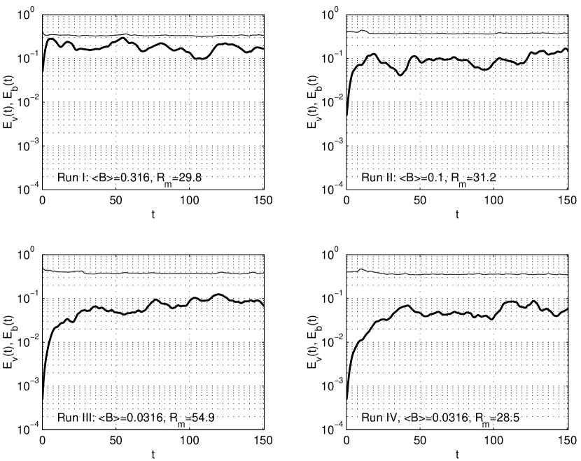
Figure 1: Temporal evolution of the kinetic energy density(thin solid line) and magnetic energy density(thick solid line) for a few run cases.

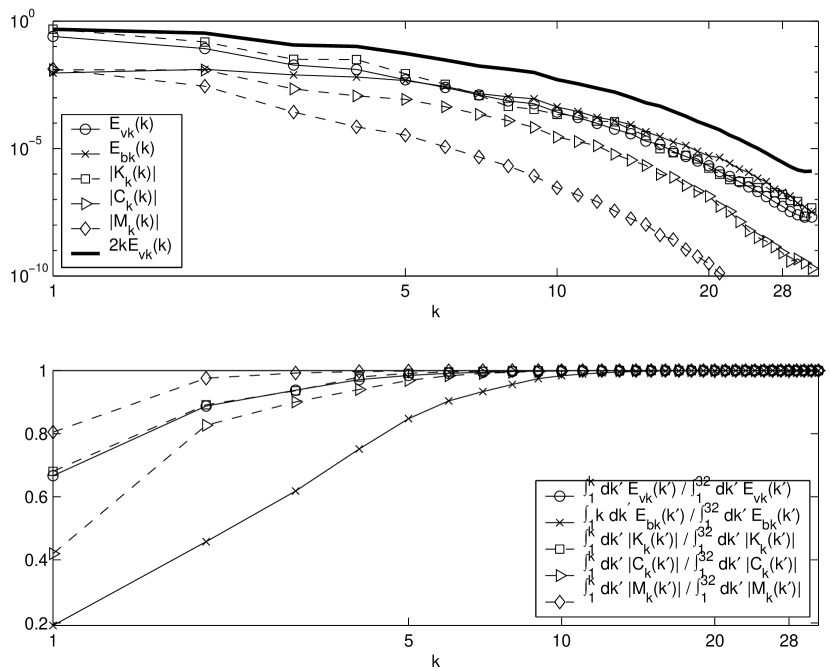
Figure 2: Top panel: kinetic energy spectrum, $E_{vk}(k)=\frac{1}{2}\sum_{k-0.5}^{k+0.5}|{\hat{v}}(k^{\prime})|^{2}$; magnetic energy spectrum, $E_{bk}(k)=\frac{1}{2}\sum_{k-0.5}^{k+0.5}|{\hat{b}}(k^{\prime})|^{2}$; absolute value of the kinetic helicity spectrum, where $K_{k}(k)=\sum_{k-0.5}^{k+0.5}\mbox{i}{\bf k}^{\prime}\cdot({\hat{\bf v}}({\bf k}^{\prime})\times{\hat{\bf v}}^{*}({\bf k}^{\prime}))$; absolute value of current helicity spectrum, where $C_{k}(k)=\sum_{k-0.5}^{k+0.5}\mbox{i}{\bf k}^{\prime}\cdot({\hat{\bf b}}({\bf k}^{\prime})\times{\hat{\bf b}}^{*}({\bf k}^{\prime}))$; absolute value of magnetic helicity spectrum, where $M_{k}(k)=\sum_{k-0.5}^{k+0.5}({\hat{\bf a}}({\bf k}^{\prime})\cdot{\hat{\bf b}}^{*}({\bf k}^{\prime}))$ and ${\bf a}$ is the vector potential of ${\bf b}$; kinetic helicity spectrum of maximally helical flow, $2kE_{vk}(k)$. Relative error for $E_{vk}(k)$ ranges from $\pm 5\%$ to $\pm 40\%$ for different $k$’s, with $k=1$ has the smallest error. Relative error for $E_{bk}(k)$ ranges from $\pm 30\%$ to $\pm 50\%$. Bottom panel: cumulative spectra of $E_{vk},E_{bk},|K_{k}|,|C_{k}|$ and $|M_{k}|$. Data are collected from Run II, averaged from time $t=52.5$ to $t=100.5$. For this case, $\langle L\rangle=0.80\pm 0.02$, $v_{rms}=0.498\pm 0.008$; therefore Reynolds number is $R_{e}=R_{m}=29.8\pm 0.9$.

To simplify matters, we set $\nu=\lambda$ in all our simulation runs, i.e., the magnetic Prandtl number is 1. $\nu(=\lambda)$ and ${\overline{{\bf B}}}$ are taken as free parameters of the numerical simulation and set up as initial conditions. All our simulation runs are performed on a $(64)^{3}$ spatial resolution. As the MHD turbulence reaches steady state, we calculate the Reynolds number of the turbulence with the formula $R_{e}(=R_{m})=\langle L\rangle v_{rms}/\nu$, where $\langle L\rangle$ is the integral length scale of the system. If $E_{vk}$ is the kinetic energy spectrum, $L$ is calculated as $\langle L\rangle=\sum_{k}k^{-1}E_{vk}/\sum_{k}E_{vk}$. At $t=0$, we impose a $\overline{{\bf B}}={\overline{B}}{\hat{\bf y}}$ into a fully developed hydrodynamic turbulence, and follow the MHD turbulence thereafter. We calculate the $\alpha$ coefficient through $\alpha=\langle{\bf v}\times{\bf b}\rangle_{y}/{\overline{B}}$. Table 1 lists all the simulation runs that we obtained. In Figure 1, we plot the evolution of kinetic energy and magnetic energy. During the kinematic phase of the development, for the first few eddy turnover times, magnetic energy density grows as $\sim t^{2}$, followed by an exponential growth. The growing magnetic energy density will impose Lorentz force on the velocity field. The kinematic phase ends when the Lorentz force is strong enough to significantly change the velocity field, and magnetic energy growth slows down. There is then a dynamic phase during which the magnetic energy and the kinetic energy oscillate around a certain level. During this phase, we can estimate the rms values of both the velocity field and the magnetic field. They are calculated using the formulae $v_{rms}=\sqrt{2E_{v}/3}$ and $b_{rms}=\sqrt{2E_{b}/3}$, where $E_{v}$ and $E_{b}$ are the kinetic energy density and magnetic energy density. In Figure 2, we plot the kinetic and magnetic energy spectra for the case of ${\overline{B}}=0.1$. At scales of $k<5$, the kinetic energy density surpasses the magnetic energy density, showing that near the outer scales, the turbulence is largely hydrodynamic in nature. For $k\geq 5$, the kinetic energy density is smaller than the magnetic energy density by a factor less than three. We also plot the spectra of the absolute values of the kinetic helicity spectrum $K_{k}$, the current helicity spectrum $C_{k}$ and the magnetic helicity spectrum $M_{k}$ (see the caption of Figure 2 for detailed definition of these spectra). In our simulation, we always force maximally (negative) helical flow within shell $S_{1}:0.5<|{\bf k}|\leq 1.5$. This explains the relation $2E_{vk}(k=1)=|K_{k}(k=1)|$ in the plot. For $k>1$, the flow is not maximally helical. Rather, $K_{k}$ decreases as $k$ increases in a way similar to $E_{vk}$, as it decays into small scales (large $k$). The current helicity, $C_{k}$, is also concentrated at large scales, $k\sim 1$, and decreases as $k$ increases. In all of our simulation runs, we find that 90% of each of the kinetic helicity, the current helicity and the magnetic helicity are concentrated near the outer scales of the turbulence, i.e., $k\leq 4$. In deriving relations (23) and (27), we assumed that magnetic helicity and current helicity are both concentrated near the outer scales of the turbulence, and approximated the total magnetic helicity and the total current helicity with $2Lb_{rms}^{2}$ and $b_{rms}^{2}/L$, respectively. From our simulation we find that such assumptions are justified, and adopt $L\sim\langle L\rangle$. Our assumption of $v_{rms}^{2}\sim b_{rms}^{2}$ is not valid for all of the cases. Therefore, when comparing our estimation of the suppressed dynamo $\alpha$ coefficient (equation (27)) with the result of numerical works (for example, Cattaneo & Hughes (1996)), we must take this factor into account.

To study the relation between the dynamo $\alpha$-effect and the dynamics of magnetic helicity, we re-write equation (17) in the form

$$2\langle{\bf v}\times{\bf b}\rangle\cdot\overline{{\bf B}}+2\lambda\langle{\bf b}\cdot\nabla\times{\bf b}\rangle+\frac{\partial}{\partial t}\langle{\bf a}\cdot{\bf b}\rangle=0.$$ (39)

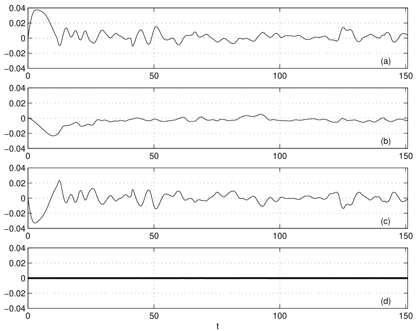
Figure 3: Temporal evolution of the following quantities: (a) $2\langle{\bf v}\times{\bf b}\rangle\cdot\overline{{\bf B}}$; (b) $2\lambda\langle{\bf b}\cdot\nabla\times{\bf b}\rangle$; (c) $\partial_{t}\langle{\bf a}\cdot{\bf b}\rangle$; (d) sum of above three quantities. Data are collected from Run I.

We calculated the numerical results of each of the three quantities and the sum of them, and plotted them in Figure 3. Panel (a) of Figure 3 is the temporal evolution of the quantity $2\langle{\bf v}\times{\bf b}\rangle\cdot\overline{{\bf B}}$. The evolution of this quantity can be separated into two stages. For $t\leq 11$, it first increases from 0 to a peak value of 0.28, then decreases until it changes sign at $t\sim 11$. After $t\sim 11$, it oscillates around an averaged value of $0.0027\pm 0.0047$. The second term in equation (39), $2\lambda\langle{\bf b}\cdot\nabla\times{\bf b}\rangle$, is plotted in panel (b) of Figure 3 with $\lambda=0.0133$. This term represents the dissipation effect. It is a less dominant effect than the dynamo $\alpha$-effect, which is represented by the first term in equation (39) and plotted in panel (a). The third term in equation (39), $\partial_{t}\langle{\bf a}\cdot{\bf b}\rangle$, is plotted in panel (c) of Figure 3. Its temporal behavior is similar to $2\langle{\bf v}\times{\bf b}\rangle\cdot\overline{{\bf B}}$. The sum of all these three quantities should be zero for our closed system with periodic boundary condition, and this is shown in the bottom panel of Figure 3.

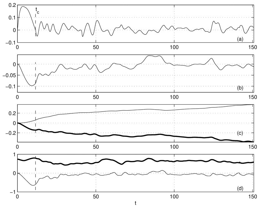
Figure 4: Panel (a): $\alpha(t)=\frac{\langle{\bf v}\times{\bf b}\rangle\cdot\overline{{\bf B}}}{{\overline{B}}^{2}}$. Panel (b): magnetic helicity density $\langle{\bf a}\cdot{\bf b}\rangle$. Panel (c): $-\int_{0}^{t}2\alpha(\tau){\overline{B}}^{2}d\tau$(thick solid line) and $-2\int_{0}^{t}\eta\langle{\bf b}\cdot\nabla\times{\bf b}\rangle$(thin solid line). Panel (d): negative kinetic helicity density, $-\langle{\bf v}\cdot\nabla\times{\bf v}\rangle$(thick solid line); current helicity density, $\langle{\bf b}\cdot\nabla\times{\bf b}\rangle$(thin solid line). $t_{c}\sim 11$. Data are collected from Run I.

We calculated the $\alpha$ coefficient with $\alpha(t)=\langle{\bf v}\times{\bf b}\rangle\cdot\overline{{\bf B}}/{\overline{B}}^{2}$ and plotted it in the top panel of Figure 4. The evolution of the small-scale magnetic helicity density, $\langle{\bf a}\cdot{\bf b}\rangle$, is shown in the middle panel of Figure 4. The initial value of the small-scale magnetic helicity is assumed to be zero. After the start of simulation, negative small-scale magnetic helicity is built up by the $\alpha$-effect with positive $\alpha$-coefficient. The speed of this building-up process achieves its maximal value when the $\alpha$-coefficient reaches its peak value. After that, the build up of negative small-scale magnetic helicity slows down as the $\alpha$-coefficient decreases. As the positive $\alpha$-coefficient approaches zero, the second term in equation (39), will dominate the $\alpha$ effect term to affect the dynamics of magnetic helicity. Panel (b) of Figure 4 and panel (b) of Figure 3 together show that when the dissipation term becomes important, the negative magnetic helicity decays. Our estimation of $\alpha(t<t_{c})$ is $0.12\pm 0.06$, and that of $\alpha(t>t_{c})$ is $0.008\pm 0.011$. This clearly shows that the dynamo $\alpha$-effect is a time-dependent quantity, and the constraint of magnetic helicity does not take effect on $\alpha$ until the building-up process of magnetic helicity is almost finished.

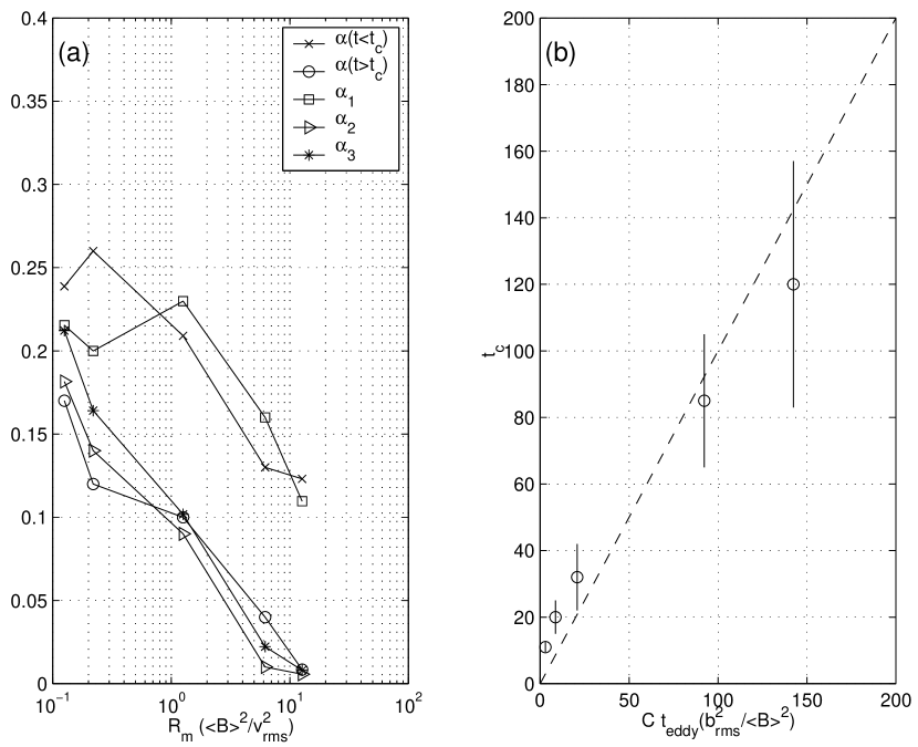
Figure 5: Panel (a): The measured $\alpha(t<t_{c})$, $\alpha(t>t_{c})$, and estimates of $\alpha$ based on different theoretical models (see text for details). Panel (b): the critical time $t_{c}$ measured from the simulation vs. the estimate based on our model (see section 1 of main text). The correction factors to $t_{c}$ are estimated by reading the spectrum of magnetic helicity and calculating the ratio $v_{rms}/\alpha_{FBC}$. The correction factors are $C=1.5,2,1,2.5$ and $3$ for Runs I to V. Error bars shown in panel (b) are the standard deviation of our calculations for $t_{c}$. For the statistical standard deviation calculations of other quantities in this figure, the reader is referred to Table I for more details.

To test how close the estimates by the models of $\alpha_{1}$, $\alpha_{2}$ and $\alpha_{3}$ to the measured $\alpha$-coefficient from our numerical simulation, we take $R=R_{m}\left({\overline{B}}^{2}/v_{rms}^{2}\right)$ as a variable, and plot the measured $\alpha$ and the estimates of $\alpha$ from different models against this quantity. The results are given in Figure 5. In panel (a) of Figure 5, we plot $\alpha(t<t_{c})$, $\alpha(t>t_{c})$, $\alpha_{1}$, $\alpha_{2}$ and $\alpha_{3}$ vs. $R$. It is clear that $\alpha(t<t_{c})$ is close to $\alpha_{1}$ for all the values of $R$ considered in our simulation runs, while $\alpha_{2}$ and $\alpha_{3}$ underestimated $\alpha(t<t_{c})$ for large values of $R$. For $R<1$, $\alpha_{1}$ and $\alpha_{2}$ give similar results. Panel (a) of this figure also shows that $\alpha_{2}$ and $\alpha_{3}$ give much better estimates of the $\alpha$-coefficient for $t>t_{c}$, when the constraint of magnetic helicity on the dynamo $\alpha$-effect finally enters. Panel (b) of Figure 5 shows a clear linear correlation between the measured critical time $t_{c}$ and our estimate of this quantity using $t_{eddy}\left(b_{rms}/{\overline{B}}\right)^{2}$, which we discussed previously in the Introduction section.

4 Discussion

The appearance of the electromotive force term in the equations for small-scale and large-scale magnetic helicity, i.e., (8) and (11), shows that the dynamo $\alpha$-effect is related to the dynamics of magnetic helicity. But because the dynamo effect is not only determined by the induction equation but also the momentum equation of the velocity field, the external forcing term in the momentum equation will provide extra degrees of freedom to the dynamo $\alpha$-effect, so that it is not completely determined by the dynamics of magnetic helicity. Instead, as we have shown in previous sections, the dynamo $\alpha$-effect is largely controlled by the velocity field during the stage that small-scale magnetic helicity of appropriate sign is being pumped into large scales. At the same time as the small-scale magnetic helicity is being pumped to large scales at this stage, the small-scale magnetic helicity of opposite sign will be built up. For closed astrophysical systems of very small magnetic diffusivity, such pumping process is in fact controlled by the dynamo $\alpha$-effect, multiplied by ${\overline{B}}^{2}$. If the initial large scale field ${\overline{B}}_{0}$ is very weak, the critical time $t_{c}=t_{eddy}\left(b_{rms}/{\overline{B}}_{0}\right)^{2}$ is initially very long, so the dynamical value of the $\alpha$-effect, i.e., $\alpha_{1}$ of PFL and FBC, applies, and considerable amplification of ${\overline{B}}$ takes place.

The Galaxy provides an interesting example. There, $t_{eddy}\sim 10^{7}$ years, $b_{rms}\sim 3\times 10^{-6}$ Gauss, and ${\overline{B}}_{0}$ has been estimated as $10^{-13}$ Gauss (Field 1994). Hence initially $t_{c}\sim 10^{22}$ years, and dynamo action is not significantly affected by the build up of magnetic helicity.

During this period, ${\overline{B}}$ will increase exponentially due to the interaction of the $\alpha$ effect and the $\omega$ effect associated with the differential rotation of the Galaxy. To avoid the complications of the $\omega$ effect here, we will consider the simpler case of an ${\alpha}^{2}$ dynamo, whose $e$-folding time is $\tau=\lambda/2\pi\alpha$. With a wavelength of 1Kpc and an $\alpha=3\times 10^{4}$cm/sec (Field 1994), $\tau=5\times 10^{8}$ years, or 50 $t_{eddy}$. Presumably growth will continue until $\tau$ matches the ever decreasing value of $t_{c}$. This will occur when ${\overline{B}}=b_{rms}/50^{2}=5\times 10^{-7}$ Gauss, after which further growth will be inhibited by the helicity constraint. To reach this stage will take 15 growth times, or $7.5\times 10^{9}$ years. Thus, during a relatively long period, dynamo growth can occur unconstrained by magnetic helicity, and during this period, can approach equipartition within an order of magnitude.

Bear in mind that this example is oversimplified. In particular, it does not take into account that helicity may escape through the boundaries of the system (Blackman & Field 2000). In this case, the boundary terms ${\bf f}$ and ${\bf F}$ in equations (14) and (15) must be taken into account, and so one must be cautious about applying conclusions from simple models like we have discussed to real astrophysical systems.

The constraint of magnetic helicity on the dynamo $\alpha$-effect, as discussed by Gruzinov & Diamond (1994, 1995, 1996), Cattaneo & Hughes (1996) and Seehafer (1994, 1995), plays important role in controlling the amount of magnetic helicity pumped by the dynamo $\alpha$-effect from small scales to large scales. It is found in this paper that such constraining effect takes place after the magnetic helicity development reaches a critical time, $t_{c}$. Before $t_{c}$, we believe that the source of magnetic helicity being pumped from small scales to large scales may not be restricted to the Ohmic dissipation at small scales. Rather, it may come from the twisting, folding and stretching of the magnetic field lines by the velocity field at different scales. Such interactions between ${\bf v}$ and ${\bf b}$ alter the topology of the magnetic field in such a way that net magnetic helicity, which represents the magnetic field line topology (Moffatt & Tsinober 1992), can be built up. Another source of magnetic helicity can be from outside of the system if there are open boundaries. During such non-stationary stage, induction equation (6) alone cannot give a complete picture of the dynamo $\alpha$-effect, and the dynamical studies by PFL and FBC may provide a valid $\alpha$-coefficient, $\alpha_{1}$, which cannot be equated to $\alpha_{2}$. When the building up of magnetic helicity approached its upper limit set by the realizability condition (22), the dynamical pumping effect described by $\alpha_{1}$ starts to be constrained by the magnetic helicity conservation. Eventually, if the system is closed, $\alpha_{1}$ alone (in the form of relation (2)) is not enough for a complete picture of the dynamo $\alpha$-effect, and $\alpha_{2}$ must be introduced to get $\alpha_{3}$.

Another motivation of our work is the numerical study of magnetic helicity by Stribling et al. (1994). In their simulation, they find that the electromotive force is not suppressed for the first few eddy turnover times in a 3D MHD turbulence with an imposed moderately strong large-scale magnetic field and an $R_{m}\rightarrow\infty$. Our work is an extension of the work by Stribling et al. in the following aspects: first, we introduced a critical time to separate the non-suppressed stage from the suppressed stage of the $\alpha$-effect; second, we numerically studied the dependence of the $\alpha$-coefficient on the values of $\overline{B}$, $b_{rms}$, $\tau_{eddy}$ and other quantities of the MHD turbulence. By doing so, we argued that the time behavior of the magnetic helicity dynamics plays an important role in the dynamo $\alpha$-effect; therefore, one cannot simply ignore the $\partial_{t}$-terms when applying the magnetic helicity equations, (17) and (18), to real astrophysical systems.

5 Conclusion

We studied the constraint of magnetic helicity on the dynamo $\alpha$-effect with 3D direct numerical simulation under periodic boundary conditions. The dynamics of magnetic helicity affects the dynamo $\alpha$-effect only after the magnetic helicity at small scales is built up and the magnetic helicity dynamics enters a stationary state. Such building-up process can be understood as a pumping effect of the dynamo $\alpha$-effect, and the $\alpha$-coefficient during this non-stationary pumping stage can be estimated according to the model by Pouquet et al. (1976) or Field et al. (1999). As the small-scale magnetic helicity is built up to the level limited by the realizability condition, the $\alpha$-effect is quenched, as suggested by Gruzinov & Diamond (1994, 1995, 1996) and Cattaneo & Hughes (1996). The $\alpha$-coefficient during such magnetic helicity constraining stage can be estimated according to the model by Seehafer (1994, 1995, see also Blackman & Field 2000). A critical time, $t_{c}\sim t_{eddy}\left(b_{rms}/{\overline{B}}\right)^{2}$, is introduced to separate these two stages.

Table 1: Measurements of various physical quantities for different simulation runs

	Run I	Run II	Run III	Run IV	Run V
${\overline{B}}$	0.316	0.1	0.0316	0.0316	0.224
$\nu(=\lambda)$	0.0133	0.0133	0.0071	0.0133	0.0133
$v_{rms}$	$0.473\pm 0.006$	$0.498\pm 0.008$	$0.50\pm 0.01$	$0.487\pm 0.005$	$0.489\pm 0.002$
$b_{rms}$	$0.35\pm 0.04$	$0.26\pm 0.04$	$0.24\pm 0.07$	$0.19\pm 0.05$	$0.27\pm 0.07$
$R_{m}$	$29.8\pm 0.9$	$31.2\pm 1.4$	$54.9\pm 2.1$	$28.5\pm 0.6$	$29.6\pm 0.9$
$t_{eddy}$	$1.6\pm 0.1$	$1.6\pm 0.2$	$1.6\pm 0.7$	$1.7\pm 0.4$	$1.7\pm 0.2$
$\tau_{cor}$	$0.64\pm 0.08$	$0.8\pm 0.3$	$0.7\pm 0.4$	$0.5\pm 0.2$	$1.0\pm 0.4$
$t_{c}$	$\sim 11$	$\sim 32$	$\sim 85$	$\sim 120$	$\sim 20$
$\alpha(t<t_{c})\tablenotemark{a}$	$0.12\pm 0.06$	$0.21\pm 0.08$	$0.26\pm 0.09$	$0.24\pm 0.26$	$0.13\pm 0.09$
$\alpha(t>t_{c})\tablenotemark{a}$	$0.008\pm 0.011$	$0.10\pm 0.11$	$0.20\pm 0.09$	$0.17\pm 0.22$	$0.04\pm 0.02$
$\alpha_{1}$	$0.11\pm 0.05$	$0.23\pm 0.05$	$0.16\pm 0.12$	$0.22\pm 0.05$	$0.16\pm 0.0.01$
$\alpha_{2}$	$0.006\pm 0.006$	$0.11\pm 0.07$	$0.14\pm 0.05$	$0.18\pm 0.17$	$0.01\pm 0.01$
$\alpha_{3}$	$0.007\pm 0.003$	$0.09\pm 0.03$	$0.13\pm 0.04$	$0.19\pm 0.06$	$0.022\pm 0.002$

References

- (1) Bhattacharjee, A. & Yuan, Y., 1995, ApJ, 449, 739
- (2) Blackman, E.G., & Field, G. 2000, ApJ, 534, 984
- (3) Brandenburg, A. 2000, astro-Ph/0006186 v2
- (4) Cattaneo, F. & Hughes, D. W. 1996, Phys. Rev. E., 54, 4532
- (5) Cattaneo, F. & Vainshtein, S.I. 1991, ApJ, 376, L21
- (6) Chen, S., Doolen, G. D., Kraichnan, R. H. & She, Z-S, Phys. Fluids, A, 5(2), 458
- (7) Cho, J. & Vishniac, E. T. 2000, preprint, astro-Ph/0003404
- (8) Field, G. B. 1994, in International Conference on Plasma Physics, ICCP 1994 (AIP Conference Proceedings 345), p. 416
- (9) Field, G. B., Blackman, E. G. & Chou, H. 1999, ApJ, 513, 638 (referred to as FBC)
- (10) Gruzinov, A. & Diamond, P. 1994, Phys. Rev. Lett., 72, 1651
- (11) Gruzinov, A. & Diamond, P. 1995, Phys. Plasmas, 2, 1651
- (12) Gruzinov, A. & Diamond, P., 1996, Phys. Plasmas, 3, 1853
- (13) Machiels, L. & Deville, M. O., 1998, J. Comput. Phys., 145, 246
- (14) Moffatt, H.K. 1978, Magnetic Field Generation in Electrically Conducting Fluids (Cambridge:Cambridge University Press)
- (15) Moffatt, H. K. & Tsinober, A. 1992, Ann. Rev. Fluid Mech., 24, 459
- (16) Krause, F. & Rädler, K.H., 1980, Mean-Field Magnetohydrodynamics and Dynamo Theory (Oxford: Pergamon)
- (17) Kulsrud, R. M. 1999, Ann. Rev. Astron. Astrophys., 37, 37
- (18) Parker, E. N. 1955, ApJ, 122, 293
- (19) Pouquet, A., Frisch, U., & Léorat, J. 1976, J. Fl. Mech., 77, pt. 2, 321 (referred to as PFL)
- (20) Seehafer, N. 1994, Europhys. Lett., 27, 353
- (21) Seehafer, N. 1995, A. & A., 301, 290
- (22) Steenbeck, M., Krause F. & Rädler, K.H., 1966, Z. Naturforsch, 21a, 369
- (23) Stribling T., Matthaeus, W. H. & Ghosh, S., 1994, J. Geophys. Res., 99, No. A2, 2567
- (24) Vainshtein, S.I. & Cattaneo, F. 1992, ApJ, 393, 165
- (25) Zeldovich, Ya. B. 1957, Sov. Phys. JETP, 4, 460