On the APM power spectrum and the CMB anisotropy: Evidence for a phase transition during inflation?

Abstract

Adams et al. (1997b) have noted that according to our current understanding of the unification of fundamental interactions, there should have been phase transitions associated with spontaneous symmetry breaking during the inflationary era. This may have resulted in the breaking of scale-invariance of the primordial density perturbation for brief periods. A possible such feature was identified in the power spectrum of galaxy clustering in the APM survey at the scale $k\sim 0.1\,h\,{\rm Mpc}^{-1}$ and it was shown that the secondary acoustic peaks in the power spectrum of the CMB anisotropy should consequently be suppressed. We demonstrate that this prediction is confirmed by the recent Boomerang and Maxima observations, which favour a step-like spectral feature in the range $k\sim(0.06-0.6)h\,{\rm Mpc}^{-1}$, independently of the similar previous indication from the APM data. Such a spectral break enables an excellent fit to both APM and CMB data with a baryon density consistent with the BBN value. It also allows the possibility of a matter-dominated universe with zero cosmological constant, which we show can now account for even the evolution of the abundance of rich clusters.

1 Introduction

It is commonly assumed by astronomers that inflation predicts a scale-invariant ‘Harrison-Zeldovich’ (H-Z) spectrum of scalar density perturbations, $\delta_{\rm H}^{2}(k)\propto\,k^{n-1}$ with $n=1$; for example this is a standard input in calculations of the expected large-scale structure (LSS) and cosmic microwave background (CMB) anisotropy. In fact in the usual ‘slow-roll’ inflationary scenario there is a gradual steepening of the spectrum with increasing $k$ (decreasing scale), as the end of inflation is approached [Mukhanov & Chibisov 1981, Hawking 1982, Starobinsky 1982, Guth & Pi 1982, Bardeen, Steinhardt & Turner 1983]. This cannot be adequately modelled by a spectrum with constant “tilt” ($n<1$) as is occasionally adopted, since the steepening is scale-dependent for any polynomial inflaton potential. Even such small departures from scale-invariance can be quite significant, for example in a supergravity model with a cubic inflaton potential, Adams, Ross & Sarkar (1997a) found $n\simeq(N-2)/(N+2)$, where $N\sim 51+\ln(k^{-1}/3000\,h^{-1}{\rm Mpc})$ is the number of e-folds of expansion from the end of inflation. This gradual suppression of small-scale power was shown to be adequate to reconcile the COBE-normalised standard cold dark matter (sCDM) model with LSS data, in particular the power spectrum of galaxy clustering, $P(k)$, the abundance of rich clusters quantified by the parameter $\sigma_{8}$, and large-scale streaming velocities, $\sigma_{v}(40\,h^{-1}{\rm Mpc})$. We emphasise that this model is however ruled out by the same data if a scale-invariant spectrum is assumed [Efstathiou, Bond & White 1992]. Such conclusions are clearly not robust given that we have as yet no standard model of inflation.

Subsequently it was realized [Adams, Ross & Sarkar 1997b] that the spectrum may not be even scale-free because the rapid cooling of the universe during primordial inflation can result in spontaneous symmetry breaking phase transitions which may interrupt the slow roll of the inflaton field for brief periods. This is in fact inevitable in models based on $N=1$ supergravity, the phenomenologically successful extension of the Standard Model of particle physics and the effective field theory below the Planck scale. During inflation, the large vacuum energy breaks supersymmetry giving otherwise massless fields (‘flat directions’) a mass of order the Hubble parameter [Dine et al. 1984, Coughlan et al. 1984], causing them to evolve rapidly to the asymmetric global minima of their scalar potential. Such ‘intermediate scale’ fields are generic in models derived from superstring/M-theory and have gauge and Yukawa couplings to the thermal plasma so are initially confined at the symmetric maxima of their scalar potentials. Consequently it takes a (calculable) finite amount of cooling before the thermal barrier disappears and they are free to evolve to their minima [Yamamoto 1986, Barreiro et al. 1996]. When a symmetry breaking transition occurs, the mass of the inflaton field changes suddenly (through couplings in the Kähler potential), temporarily violating the slow-roll conditions and interrupting inflation (Adams et al. 1997b). Thus the density perturbation is expected to have a (near) H-Z spectrum for the first $\sim 10$ e-folds of expansion followed by one or more sudden departures from scale-invariance lasting $\sim 1$ e-fold. In order for such spectral features to be observable in the LSS or CMB, it is of course necessary that they occur within the last $\sim 50$ e-folds of inflation, corresponding to spatial scales going up to the present Hubble radius $H_{0}^{-1}\sim 3000\,h^{-1}{\rm Mpc}$. Since the density perturbation can be observed on scales from the Hubble radius down to $\sim 1\,h^{-1}{\rm Mpc}$, corresponding to about 8 e-folds of expansion, it would be not unreasonable to expect at least one such spectral break to be seen today.

Motivated by this an attempt was made to recover the primordial perturbation spectrum from extant observations of LSS and CMB anisotropy, specifically the APM survey [Maddox et al. 1990a] and the COBE observations [Smoot et al. 1992]. We recall that the spectrum of rms mass fluctuations at the present epoch (per unit logarithmic interval of wavenumber $k$) is

$$\Delta^{2}(k)\equiv\frac{k^{3}P(k)}{2\pi^{2}}=\delta^{2}_{\rm H}(k)\ T^{2}(k)\left(\frac{k}{H_{0}}\right)^{3+n}\ ,$$ (1)

where the density perturbation is evaluated at the present Hubble radius, i.e. at $k=H_{0}$. The (dimensionless) matter ‘transfer function’ for CDM models can be approximated by [Bond & Efstathiou 1984]

$$T_{{\rm CDM}}(k)\simeq\left[1+\left\{ak+(bk)^{3/2}+(ck)^{2}\right\}^{\nu}\right]^{-1/\nu}\ ,$$ (2)

with $a=6.4\Gamma^{-1}\,h^{-1}{\rm Mpc}$, $b=3\Gamma^{-1}\,h^{-1}{\rm Mpc}$, $c=1.7\Gamma^{-1}\,h^{-1}{\rm Mpc}$ and $\nu=1.13$. Here the ‘shape parameter’ is defined as [Bond & Jaffe 1999]

$$\Gamma=\Omega_{\rm m}{h}{\rm e}^{-[\Omega_{\rm B}(1+\sqrt{2h}/\Omega_{\rm m})-0.06]},$$ (3)

where $h\equiv\,H_{0}/100\,{\rm Km\,s}^{-1}{\rm Mpc}^{-1}$ is the Hubble parameter and $\Omega_{\rm m}=\Omega_{\rm CDM}+\Omega_{\rm B}$, $\Omega_{\rm CDM}$ ($\Omega_{\rm B}$) being the fraction of the critical density in cold (baryonic) matter. Thus $\Gamma=0.5$ for sCDM which assumes $\Omega_{\rm B}=0.03$, $\Omega_{\rm m}=1$ and $h=0.5$.

Following Baugh & Gaztañaga (1996), the three-dimensional $P_{{\rm APM}}(k)$ inferred from the angular correlation function of galaxies in the APM survey [Baugh & Efstathiou 1993] was subjected to an inversion procedure [Jain, Mo & White 1995, Peacock & Dodds 1996] to recover the linear spectrum of fluctuations and obtain its spectral index, ${\rm d}\ln{P(k)}/{\rm d}\ln{k}$, as a function of $k$. Assuming that any bias between APM galaxies and dark matter is scale-independent, the primordial spectral index $n(k)$ was then obtained simply by subtracting off the slope of the transfer function (2) for each value of $k$ (Adams et al. 1997b).

The key finding was that $n_{{\rm APM}}(k)$ shows a dramatic departure from the H-Z value of $n=1$ in the range $k\sim(0.05-0.6)h\,{\rm Mpc}^{-1}$, dropping to a value around zero ($\sim 3\sigma$ below unity) at $k\sim 0.1\,h\,{\rm Mpc}^{-1}$. The sharp drop occurs over $\sim 1$ e-fold of expansion as is indeed expected in the phase transition model. This feature in $P_{{\rm APM}}(k)$ had been noted by Baugh & Efstathiou (1993) and was also identified by Peacock (1997) in the power spectrum of IRAS galaxies after correcting for redshift-space distortions. Given that the feature appears on the scale of the Hubble radius at the epoch of (dark) matter domination, it is perhaps natural to interpret it as reflecting a departure from the sCDM paradigm as these authors did. However Adams et al. (1997b) pursued the alternative possibility that it is in fact present in the primordial spectrum and asked what would be the expectation for the angular anisotropy of the CMB if this were so. Using the COSMICS code [Bertschinger 1995] they calculated its angular power spectrum and found that the height of the secondary acoustic peaks is suppressed by a factor of $\sim 2$ relative to the prediction of the standard COBE-normalised sCDM model which assumes a scale-free H-Z spectrum.

We reexamine this prediction in the light of recent observations by the Boomerang [de Bernadis et al. 2000] and MAXIMA-1 [Hanany et al. 2000] experiments which do indicate a significant suppression of the second acoustic peak. It has been noted by many authors [Tegmark & Zaldarriaga 2000, Lange et al. 2001, Balbi et al. 2000, Hu et al. 2000, Jaffe et al. 2000, Esposito et al. 2001, Padmanabhan & Sethi 2000] that this requires a high baryon density, significantly above the value required by light element abundances following from standard Big Bang nucleosynthesis (BBN). As the latter is widely considered to be one of the “pillars” of modern cosmology, it is important to ask whether this conflict may not be resolved by relaxing the assumption made in these analyses that the primordial spectrum of perturbations is scale-free.

2 Reconstructing the primordial spectrum

We begin by describing the range of values that we consider for the cosmological parameters. This represents the set of priors, resulting from other observations, that we adopt for the reconstruction of the primordial spectrum. In §2.2, we discuss how LSS data can be used to recover the primordial spectrum and predict the CMB anisotropy (§2.3). In §2.4 we present a simple parameterization for the primordial spectrum and use this to fit the new CMB as well as APM data. Finally in §2.5 we confront the observed abundance of rich clusters with the expectations in our model.

2.1 Cosmological parameters

Let us first briefly discuss the choice of cosmological parameters. As mentioned before, $\Gamma=0.5$ in the sCDM model, but $\Gamma\simeq 0.2$ gives in fact a better fit to the APM data [Maddox et al. 1990b, Efstathiou, Bond & White 1992, Baugh & Efstathiou 1993, Peacock & Dodds 1994] and can be realized e.g. in a low density model with $\Omega_{\rm m}\sim 0.4$. The alternative possibility of a Hubble parameter as low as $h\sim 0.3$ [Bartlett et al. 1995] is definitively ruled out by the HST Key Project data on 25 galaxies which indicates $h=0.71\pm 0.06$ [Mould et al. 2000]. Weighting such direct observations against other fundamental physics approaches, Primack (2000) advocates $h=0.65\pm 0.08$. However a value as low as 0.45 [Parodi et al. 2000] or as high as 0.9 [Tonry et al. 2000] still seems quite possible so the quoted uncertainty cannot be interpreted as a gaussian standard deviation. Instead we assume that all values in the following “$2\sigma$” range are equally probable:

$$h=0.49-0.81.$$ (4)

The current preference is in fact for a cosmological constant dominated flat universe with $\Omega_{\Lambda}\simeq 2/3$ and $\Omega_{\rm m}\simeq 1/3$ (e.g. Bahcall et al. 1999). The Boomerang and MAXIMA observations of the first acoustic peak indicate that the universe is indeed flat [Jaffe et al. 2000], but we will consider other $\Lambda$CDM models with values of $\Omega_{\Lambda}$ ranging down to zero, maintaining $\Omega{\rm m}+\Omega_{\Lambda}=1$. This is motivated by our concern that the only direct evidence suggesting $\Omega_{\Lambda}\sim 0.7$ is the small curvature of the Hubble diagram for Type Ia supernovae at redshift $z\sim 1$ [Perlmutter et al. 1999, Riess et al. 1998] which may be subject to unrecognised systematic effects. (We note that other arguments for a low $\Omega_{\rm m}$ from the evolution of the cluster number density [Eke et al. 1998] or the clustering in the Lyman-$\alpha$ forest [Weinberg et al. 1999] rest on the assumption of a scale-free spectrum.) Of course for any particular choice of $(\Omega_{\rm m},\Omega_{\Lambda})$, one has to check that the age of the universe exceeds the inferred age of globular clusters, $t_{\rm GC}=12.8\pm 1$ Gyr [Krauss 2000].

Another important parameter for the present study is the BBN value of $\Omega_{\rm B}$. This has undergone substantial revision since the first studies of sCDM so we briefly review the present situation. The baryon density which provides a good fit to the inferred primordial abundances of D, ⁴He and ⁷Li in standard BBN is [Fiorentini et al. 1998]

$$\Omega_{\rm B}=(0.019^{+0.0013}_{-0.0012})h^{-2},$$ (5)

taking all (correlated) reaction rate uncertainties into account. This fit is based on the ‘low’ value of D/H=$(3.4\pm 0.25)\times 10^{-5}$ found [Burles & Tytler 1998] in two quasar absorption systems (QAS) at high redshift [and subsequently in a third one [Kirkman et al. 2000]], the ‘high’ value of the mass fraction Y(⁴He)=$0.243\pm 0.003$ inferred [Izotov, Thuan & Lipovetsky 1998] from observations of metal-poor blue compact galaxies (BCGs), and the ‘Spite plateau’ of ⁷Li/H=$(1.73\pm 0.12)\times 10^{-10}$ seen in Pop II stars [Bonifacio & Molaro 1997]. Note however that an improved fit is obtained [Fiorentini et al. 1998] at a significantly smaller value of $\Omega_{\rm B}=(0.0065^{+0.0010}_{-0.00064})h^{-2}$ if one adopts the ‘high’ value of D/H=$(1.9\pm 0.4)\times 10^{-4}$ claimed [Songaila et al. 1994] in another QAS [but disputed subsequently [Burles, Kirkman & Tytler 1999], although consistent with a possible high value [Tytler et al. 1999] in yet another QAS], and the ‘low’ value of Y(⁴He)=$0.234\pm 0.005$ obtained [Olive, Skillman & Steigman 1997] from analysis of older BCG data [and supported by another recent observation [Peimbert, Peimbert & Ruiz 2000]]. An independent lower limit of $\Omega_{\rm B}>0.0125h^{-2}$[Weinberg et al. 1997] set by observations of the Lyman-$\alpha$ forest favours the higher value in Equation (5), which also allows a better fit to the observed distribution of line widths in comparison with model hydrodynamic simulations (e.g. Theuns et al. 1999). An audit of luminous matter in the universe [Fukugita, Hogan & Peebles 1998] gives a much weaker lower limit of $\Omega_{\rm B}\mathrel{\mathchoice{\lower 3.6pt\vbox{\halign{$\mathsurround=0pt\displaystyle\hfill#\hfil$\cr>\crcr\sim\crcr}}}{\lower 3.6pt\vbox{\halign{$\mathsurround=0pt\textstyle\hfill#\hfil$\cr>\crcr\sim\crcr}}}{\lower 3.6pt\vbox{\halign{$\mathsurround=0pt\scriptstyle\hfill#\hfil$\cr>\crcr\sim\crcr}}}{\lower 3.6pt\vbox{\halign{$\mathsurround=0pt\scriptscriptstyle\hfill#\hfil$\cr>\crcr\sim\crcr}}}}0.007$. A conservative upper limit on the baryon density is [Kernan & Sarkar 1996]

$$\Omega_{\rm B}<0.033\,h^{-2},$$ (6)

if the primordial deuterium abundance is bounded from below by its typical interstellar value D/H=$(1.5\pm 0.2)\times 10^{-5}$ [McCullough 1992]. Therefore we will consider a wide range of possible values in our analysis, but adopt $\Omega_{\rm B}=0.045$, $h=0.65$ as the default values (so that $\Omega_{\rm CDM}=\Omega_{\rm m}-0.045$) when not stated otherwise.

2.2 Primordial spectrum from the APM data

There are several arguments (reviewed in Appendix A) that on scales $0.01\,h\,{\rm Mpc}^{-1}\mathrel{\mathchoice{\lower 3.6pt\vbox{\halign{$\mathsurround=0pt\displaystyle\hfill#\hfil$\cr<\crcr\sim\crcr}}}{\lower 3.6pt\vbox{\halign{$\mathsurround=0pt\textstyle\hfill#\hfil$\cr<\crcr\sim\crcr}}}{\lower 3.6pt\vbox{\halign{$\mathsurround=0pt\scriptstyle\hfill#\hfil$\cr<\crcr\sim\crcr}}}{\lower 3.6pt\vbox{\halign{$\mathsurround=0pt\scriptscriptstyle\hfill#\hfil$\cr<\crcr\sim\crcr}}}}\,k\mathrel{\mathchoice{\lower 3.6pt\vbox{\halign{$\mathsurround=0pt\displaystyle\hfill#\hfil$\cr<\crcr\sim\crcr}}}{\lower 3.6pt\vbox{\halign{$\mathsurround=0pt\textstyle\hfill#\hfil$\cr<\crcr\sim\crcr}}}{\lower 3.6pt\vbox{\halign{$\mathsurround=0pt\scriptstyle\hfill#\hfil$\cr<\crcr\sim\crcr}}}{\lower 3.6pt\vbox{\halign{$\mathsurround=0pt\scriptscriptstyle\hfill#\hfil$\cr<\crcr\sim\crcr}}}}\,0.6\,h\,{\rm Mpc}^{-1}$, which are at most weakly non-linear, the APM galaxy power spectrum $P_{\rm APM}(k)$ [Baugh & Efstathiou 1993] is an unbiased (or moderately linearly biased) tracer of the mass. The linear power spectrum recovered under this assumption from $P_{\rm APM}(k)$, using the method of Jain et al. (1995), is well fitted in this range by [Baugh & Gaztañaga 1996]:

$$P_{{\rm lin}}(k)\simeq\frac{7\times 10^{5}k\,(\,h^{-1}{\rm Mpc})^{3}}{\left[1+(k/k_{\rm c})^{2}\right]^{1.6}}\ ,$$ (7)

where $k_{\rm c}=150(H_{0}/c)\simeq 0.05\,h\,{\rm Mpc}^{-1}$. We will use the common convention of expressing the matter power spectrum as the primordial spectrum of matter fluctuations $P^{0}(k)\propto\,k\delta^{2}_{\rm H}(k)$, folded with the transfer function (2):

$$P_{\rm lin}(k)\equiv P^{0}(k)\,T^{2}(k)=Ak^{n}T^{2}(k),$$ (8)

where the (dimensionful) normalisation constant $A$ is determined by the large-scale CMB anisotropy. [For sCDM with $n=1$ normalised to the COBE 4-year data [Bennett et al. 1996], $\delta_{\rm H}=1.92\times 10^{-5}$ with 9% uncertainty [Bunn & White 1997] so $A=(5.9\pm 1.1)\times 10^{5}(\,h^{-1}{\rm Mpc})^{4}$.]

Given some estimate of the (linear) matter power spectrum, as in Equation (7), the standard approach is to assume a scale-invariant initial spectrum, i.e. $P^{0}(k)\propto\,k$, and extract the value of $\Gamma$ that best fits the resulting constraint on $T(k)$. Alternatively one can extract $P^{0}(k)(=P_{{\rm lin}}/T^{2}$) for a specific choice of $\Gamma$, i.e. for a given transfer function. We apply this latter approach to the APM data by simply taking the ratio of Equation (7) to Equation (2), obtaining:

$$P^{0}(k)=\left\{\begin{array}[]{ll}A_{1}k,&\mbox{$k<k_{1}$,}\\ Ak\frac{\left[1+(ak+(bk)^{3/2}+(ck)^{2})^{u}\right]^{2/u}}{\left[1+(k/k_{\rm c})^{2}\right]^{1.6}},&\mbox{$k_{1}\leq k\leq k_{2}$,}\\ A_{2}k,&\mbox{$k_{2}<k$,}\end{array}\right.$$ (12)

where $A=7\times 10^{5}(\,h^{-1}{\rm Mpc})^{3}$ and we have adopted a suitably normalised H-Z spectrum outside the range ($k<k_{1}=0.01\,h\,{\rm Mpc}^{-1}$, $k>k_{2}=0.6\,h\,{\rm Mpc}^{-1}$) accessible to galaxy clustering observations.

Figure 1 shows the recovered spectrum (12) for two choices of $\Gamma$ corresponding to the sCDM model and a low density variant. Note that the $\Gamma=0.5$ reconstruction has significantly less power than a scale-free H-Z spectrum on scales $k\mathrel{\mathchoice{\lower 3.6pt\vbox{\halign{$\mathsurround=0pt\displaystyle\hfill#\hfil$\cr>\crcr\sim\crcr}}}{\lower 3.6pt\vbox{\halign{$\mathsurround=0pt\textstyle\hfill#\hfil$\cr>\crcr\sim\crcr}}}{\lower 3.6pt\vbox{\halign{$\mathsurround=0pt\scriptstyle\hfill#\hfil$\cr>\crcr\sim\crcr}}}{\lower 3.6pt\vbox{\halign{$\mathsurround=0pt\scriptscriptstyle\hfill#\hfil$\cr>\crcr\sim\crcr}}}}0.1\,h\,{\rm Mpc}^{-1}$, while the $\Gamma=0.2$ reconstruction is closer to a H-Z spectrum but has relatively more power. However as we shall see the latter possibility does not give a good fit to the Boomerang/MAXIMA data with the BBN value (5) of the baryon density. To ensure compatibility with BBN requires a break in the primordial spectrum.

Figure 1: Reconstruction of the primordial density power spectrum from the APM data, adopting a CDM shape parameter $\Gamma$ of 0.5 (dot-dashed line) and 0.2 (dashed line). A Harrison-Zeldovich spectrum (full line) is shown for comparison.

2.3 Acoustic peaks

In linear theory the co-efficents $C_{l}$ in the spherical harmonics expansion of the CMB anisotropy are a linear projection of $P(k)$, so the effect of changing $P^{0}(k)$ would just be to proportionally alter the angular power for the multipoles $l$ corresponding to the relevant values of $k$. We can approximate $l\simeq\pi/\theta_{\rm LSS}$ where $\theta_{\rm LSS}\simeq\lambda/D_{\rm LSS}$ is the angular size corresponding to a comoving distance $\lambda$ at the last scattering surface (LSS), which is at a distance $D_{\rm LSS}\simeq 2(c/H_{0}\Omega_{\rm m}^{0.4})$ for a flat universe [Vittorio & Silk 1992]. Thus

$$l\simeq k/D_{\rm LSS}\simeq 3000k\Omega_{\rm m}^{-0.4}h^{-1}.$$ (13)

For the $\Gamma=0.5$ case (corresponding e.g. to $\Omega_{\rm m}=0.805$, $\Omega_{\Lambda}=0.195$) the inferred primordial power in Figure 1 is suppressed by a factor $\mathrel{\mathchoice{\lower 3.6pt\vbox{\halign{$\mathsurround=0pt\displaystyle\hfill#\hfil$\cr>\crcr\sim\crcr}}}{\lower 3.6pt\vbox{\halign{$\mathsurround=0pt\textstyle\hfill#\hfil$\cr>\crcr\sim\crcr}}}{\lower 3.6pt\vbox{\halign{$\mathsurround=0pt\scriptstyle\hfill#\hfil$\cr>\crcr\sim\crcr}}}{\lower 3.6pt\vbox{\halign{$\mathsurround=0pt\scriptscriptstyle\hfill#\hfil$\cr>\crcr\sim\crcr}}}}2$ for $k\mathrel{\mathchoice{\lower 3.6pt\vbox{\halign{$\mathsurround=0pt\displaystyle\hfill#\hfil$\cr>\crcr\sim\crcr}}}{\lower 3.6pt\vbox{\halign{$\mathsurround=0pt\textstyle\hfill#\hfil$\cr>\crcr\sim\crcr}}}{\lower 3.6pt\vbox{\halign{$\mathsurround=0pt\scriptstyle\hfill#\hfil$\cr>\crcr\sim\crcr}}}{\lower 3.6pt\vbox{\halign{$\mathsurround=0pt\scriptscriptstyle\hfill#\hfil$\cr>\crcr\sim\crcr}}}}0.1\,h\,{\rm Mpc}^{-1}$, implying a similar decrease in the CMB anisotropy at $l\mathrel{\mathchoice{\lower 3.6pt\vbox{\halign{$\mathsurround=0pt\displaystyle\hfill#\hfil$\cr>\crcr\sim\crcr}}}{\lower 3.6pt\vbox{\halign{$\mathsurround=0pt\textstyle\hfill#\hfil$\cr>\crcr\sim\crcr}}}{\lower 3.6pt\vbox{\halign{$\mathsurround=0pt\scriptstyle\hfill#\hfil$\cr>\crcr\sim\crcr}}}{\lower 3.6pt\vbox{\halign{$\mathsurround=0pt\scriptscriptstyle\hfill#\hfil$\cr>\crcr\sim\crcr}}}}500$. For the $\Gamma=0.2$ case (corresponding e.g. to $\Omega_{\rm m}=0.35$, $\Omega_{\Lambda}=0.65$), the inferred primordial spectrum is a factor of $\sim 2$ above the H-Z one at $k\simeq 0.04\,h\,{\rm Mpc}^{-1}$ so the CMB anisotropy should be proportionally boosted at $l\mathrel{\mathchoice{\lower 3.6pt\vbox{\halign{$\mathsurround=0pt\displaystyle\hfill#\hfil$\cr>\crcr\sim\crcr}}}{\lower 3.6pt\vbox{\halign{$\mathsurround=0pt\textstyle\hfill#\hfil$\cr>\crcr\sim\crcr}}}{\lower 3.6pt\vbox{\halign{$\mathsurround=0pt\scriptstyle\hfill#\hfil$\cr>\crcr\sim\crcr}}}{\lower 3.6pt\vbox{\halign{$\mathsurround=0pt\scriptscriptstyle\hfill#\hfil$\cr>\crcr\sim\crcr}}}}250$.

To check these expectations, we ran the Boltzmann code CMBFAST [Seljak & Zaldarriaga 1996] with the above reconstructed primordial spectra as well as a H-Z spectrum with the same cosmological parameters. As seen in Figure 2, the angular power resulting from the APM inversion with $\Gamma=0.5$ is indeed depressed below the H-Z case from the second acoustic peak onwards, as noted by Adams et al. (1997b). By contrast, for the $\Gamma=0.2$ reconstruction all the acoustic peaks are boosted above the H-Z case. It is clear that the recent CMB observations favour a high density universe. Moreover the observed suppression of the second acoustic peak in the Boomerang/MAXIMA data confirms the prior expectation for a primordial density perturbation with broken scale-invariance. To quantify this we now perform detailed fits to the data.

Figure 2: The predicted CMB angular power spectra corresponding to the reconstructed primordial spectra for $\Gamma=0.5$ (dot-dashed line) and $\Gamma=0.2$ (dashed line). The corresponding results for a primordial H-Z spectrum is also shown for $\Gamma=0.5$ and $\Gamma=0.2$ (thick and thin full lines). The data are from the Boomerang (crosses) and MAXIMA (diamonds) experiments.

2.4 Fits to the CMB and LSS data

We parameterise the ‘step’ in the primordial power spectrum (see Figure 1) as:

$$P^{0}(k)=\left\{\begin{array}[]{ll}Ak,&k\leq k_{\rm s}\\ Ck^{\alpha},&k_{\rm e}\leq k\leq k_{\rm s}\\ Bk,&k\geq k_{\rm e}\\ \end{array}\right.$$ (17)

where $k_{\rm s}$ and $k_{\rm e}$ mark the start and end of the break from a H-Z spectrum, with amplitudes $A$ and $B$. (The values of $C$ and $\alpha$ are specified by the other parameters.) In the multiple inflation model (Adams et al. 1997b), the actual form of the spectrum during the phase transition is difficult to calculate since the usual ‘slow-roll’ conditions are violated. However a robust expectation is that

$$0.5\mathrel{\mathchoice{\lower 3.6pt\vbox{\halign{$\mathsurround=0pt\displaystyle\hfill#\hfil$\cr<\crcr\sim\crcr}}}{\lower 3.6pt\vbox{\halign{$\mathsurround=0pt\textstyle\hfill#\hfil$\cr<\crcr\sim\crcr}}}{\lower 3.6pt\vbox{\halign{$\mathsurround=0pt\scriptstyle\hfill#\hfil$\cr<\crcr\sim\crcr}}}{\lower 3.6pt\vbox{\halign{$\mathsurround=0pt\scriptscriptstyle\hfill#\hfil$\cr<\crcr\sim\crcr}}}}\ln\left(\frac{k_{\rm e}}{k_{\rm s}}\right)\mathrel{\mathchoice{\lower 3.6pt\vbox{\halign{$\mathsurround=0pt\displaystyle\hfill#\hfil$\cr<\crcr\sim\crcr}}}{\lower 3.6pt\vbox{\halign{$\mathsurround=0pt\textstyle\hfill#\hfil$\cr<\crcr\sim\crcr}}}{\lower 3.6pt\vbox{\halign{$\mathsurround=0pt\scriptstyle\hfill#\hfil$\cr<\crcr\sim\crcr}}}{\lower 3.6pt\vbox{\halign{$\mathsurround=0pt\scriptscriptstyle\hfill#\hfil$\cr<\crcr\sim\crcr}}}}2,$$ (18)

because the field undergoing the symmetry-breaking phase transition evolves exponentially fast to its minimum. The ratio of the amplitudes $A/B$ is determined by the (unknown) superpotential couplings of the field undergoing the phase transition but is expected to exceed unity (i.e. there is a decrease in the power).

We allow the spectral and cosmological parameters to range rather widely as follows:

• $k_{\rm s}$ from (0.01–0.15) $h\,{\rm Mpc}^{-1}$

• $\ln(k_{\rm e}/k_{\rm s})$ from 0.01–4

• $A/B$ from 0.3–7.2

• $\Omega_{\Lambda}$ from 0–0.7 (keeping $\Omega_{\rm m}+\Omega_{\Lambda}=1$)

• $h$ from 0.45–0.9

• $\Omega_{\rm B}h^{2}$ from 0.0014–0.033

We also consider a bias parameter $b$, defined as the square root of the ratio of the APM and CMB normalisations (which is expected to be close to unity, see Appendix A).

For each combination of the above parameters we construct the primordial power spectrum and then obtain the matter power spectrum by convoluting with the CDM transfer function calculated by CMBFAST (which differs slightly from the analytic approximation in Equation 2). It is also used to calculate the expected CMB angular power spectrum. These are then compared, respectively, with the APM data [Gaztañaga & Baugh 1998], and the decorrelated COBE [Tegmark & Hamilton 1997] and Boomerang data [de Bernadis et al. 2000] using appropriate window functions, to determine $\chi^{2}(\alpha)=\sum_{i}[({\rm model}(\alpha)-{\rm data}(i))/\sigma(i)]^{2}$. We use 19 CMB data points [7 from COBE (excluding the anomalously low quadrupole) and 12 from Boomerang] and 10 APM data points (for $0.01\,h\,{\rm Mpc}^{-1}\mathrel{\mathchoice{\lower 3.6pt\vbox{\halign{$\mathsurround=0pt\displaystyle\hfill#\hfil$\cr<\crcr\sim\crcr}}}{\lower 3.6pt\vbox{\halign{$\mathsurround=0pt\textstyle\hfill#\hfil$\cr<\crcr\sim\crcr}}}{\lower 3.6pt\vbox{\halign{$\mathsurround=0pt\scriptstyle\hfill#\hfil$\cr<\crcr\sim\crcr}}}{\lower 3.6pt\vbox{\halign{$\mathsurround=0pt\scriptscriptstyle\hfill#\hfil$\cr<\crcr\sim\crcr}}}}{k}\mathrel{\mathchoice{\lower 3.6pt\vbox{\halign{$\mathsurround=0pt\displaystyle\hfill#\hfil$\cr<\crcr\sim\crcr}}}{\lower 3.6pt\vbox{\halign{$\mathsurround=0pt\textstyle\hfill#\hfil$\cr<\crcr\sim\crcr}}}{\lower 3.6pt\vbox{\halign{$\mathsurround=0pt\scriptstyle\hfill#\hfil$\cr<\crcr\sim\crcr}}}{\lower 3.6pt\vbox{\halign{$\mathsurround=0pt\scriptscriptstyle\hfill#\hfil$\cr<\crcr\sim\crcr}}}}0.2\,h\,{\rm Mpc}^{-1}$). We quantify the goodness-of-fit following the procedure of Lineweaver & Barbosa (1998).

In Table 1 we show the values of the Hubble constant, baryon density, and amplitude change at the spectral break which minimise the $\chi^{2}$ (for a specific choice of $\Omega_{\Lambda}$) for fits to the CMB data alone. The step in the primordial spectrum is seen to be not essential for a good fit, in particular even with $A/B=1$ (i.e. no step) the $\chi^{2}$ does not worsen significantly in most cases. The best overall fit obtains for $\Omega_{\Lambda}=0.5$, consistent with the analysis by the Boomerang collaboration [de Bernadis et al. 2000]. Note however that the baryon density required is 65% higher than the preferred BBN value (5) although still within the upper limit (6) set by interstellar deuterium.

$\Omega_{\Lambda}$	$h$	$k_{\rm s}$	$\ln\left({\textstyle\frac{k_{\rm e}}{k_{\rm s}}}\right)$	$\Omega_{{\rm B}}h^{2}$	${\textstyle\frac{A}{B}}$	$\chi^{2}$ $\left({\textstyle\frac{A}{B}}=1\right)$
0.0	0.45	0.03	0.7	0.019	$\geq$ 1.7	7.5 (30)
0.2	0.55	0.03	0.7	0.023	$\geq$ 1.4	6.9 (19)
0.3	0.75	0.05	0.8	0.031	$\geq$ 1.3	6.6 (14)
0.4	0.75	0.03	0.8	0.031	$\geq$ 1.1	6.3 ( 8)
0.5	0.80	0.02	0.6	0.031	$\geq$ 1.0	5.8 ( 6)
0.6	0.85	0.02	0.7	0.031	$\geq$ 1.0	5.5 ( 6)
0.7	0.90	0.03	1.0	0.031	0.7–0.9	7.5 (11)

Table 1: Parameters for best fits to CMB data (13 ${\rm d.o.f.}$).

$\Omega_{\Lambda}$	$h$	$k_{\rm s}$	$\ln\left({\textstyle\frac{k_{\rm e}}{k_{\rm s}}}\right)$	${\textstyle\frac{A}{B}}$	$\chi^{2}$
0.0	0.50	0.04	0.7	1.7-3.1	8.1
0.2	0.50	0.03	0.7	1.7-3.1	7.2
0.3	0.55	0.03	0.8	1.7-3.1	6.9
0.4	0.60	0.03	0.8	1.7-3.1	6.9
0.5	0.65	0.04	0.6	1.7-2.8	7.9
0.6	0.75	0.05	0.6	1.5-2.1	11.9
0.7	0.80	0.01	0.6	0.7-0.9	35.1

Table 2: Parameters for best fits to CMB data with the BBN constraint on the baryon density.

If we now demand that the models should have the BBN baryon density (5), the Hubble parameter in the range (4) and a spectral break duration (18), then a step in the primordial spectrum is definitely indicated as seen from Table 2. [In particular setting $A/B=1$ (no step) always gives an unacceptably high value of $\chi^{2}>26$.] The angular power spectra corresponding to some of these models is shown in Figure 3 along with the Boomerang and COBE data. We emphasize that a good fit is now obtained even for $\Omega_{\Lambda}=0$.

Figure 3: CMB angular power spectra for the best-fit models in Table 2, with $\Omega_{\Lambda}=0$ (continuous line), $\Omega_{\Lambda}=0.2$ (dashed line), $\Omega_{\Lambda}=0.4$ (dot-dashed line), and $\Omega_{\Lambda}=0.6$ (dotted line). The data shown are from COBE and Boomerang. All models have the BBN baryon density $\Omega_{{\rm B}}=0.019h^{-2}$.

$\Omega_{\Lambda}$	$h$	$\Omega_{{\rm B}}h^{2}$	$k_{\rm s}$	$\ln\left({\textstyle\frac{k_{\rm e}}{k_{\rm s}}}\right)$	${\textstyle\frac{A}{B}}$	$\chi^{2}$
0.0	0.50	0.019	0.07	1.5	4.3-6.5	11.9
0.2	0.60	0.023	0.07	1.4	3.7-5.6	9.4
0.3	0.65	0.023	0.07	1.4	3.6-5.5	8.2
0.4	0.70	0.023	0.07	1.4	3.2-5.0	8.3
0.5	0.85	0.031	0.08	1.2	3.1-4.6	7.5
0.6	0.90	0.031	0.07	1.3	2.4-3.6	9.0
0.7	0.90	0.023	0.06	2.0	1.6-5.1	30.4

Table 3: Parameters for best fits to CMB+APM data (22 ${\rm d.o.f.}$).

Next we fit simultaneously to both the APM and CMB data allowing for a small difference in the normalisations, i.e. a bias $b$. We have taken into account that the mean redshift of the APM galaxies is $z=0.15$ so a corresponding correction for the growth factor to $z=0$ needs to be applied. It is seen from Table 3 that the best overall fit is still obtained for $\Omega_{\Lambda}=0.5$, although other values remain quite acceptable. In particular the $\Omega_{\Lambda}=0$ model requires a Hubble parameter at the low end of the allowed range but has the advantage of being consistent with the BBN value of the baryon density. We emphasise that a break in the spectrum is now definitely required since the value of $\chi^{2}$ exceeds 45 otherwise. The most likely duration of the break also comes out in accord with the theoretical expectation (18).

$\Omega_{\Lambda}$	$h$	$k_{\rm s}$	$\ln\left({\textstyle\frac{k_{\rm e}}{k_{\rm s}}}\right)$	${\textstyle\frac{A}{B}}$	$\sigma_{8}$	$\chi^{2}$
0.0	0.50	0.07	1.5	4.3-6.5	0.65-0.73	11.9
0.2	0.55	0.06	1.6	3.6-5.6	0.69-0.78	10.0
0.3	0.60	0.06	1.6	3.4-5.0	0.76-0.85	10.3
0.4	0.65	0.05	1.5	3.1-4.6	0.77-0.87	13.1
0.5	0.70	0.05	1.6	2.6-4.1	0.81-0.93	18.8
0.6	0.75	0.05	2.0	2.0-2.8	0.90-0.99	29.7

Table 4: Parameters for best fits to CMB+APM data with the BBN constraint on the baryon density.

Figure 4: Primordial power spectra for the best-fit models in Table 4 with $\Omega_{\Lambda}=0$ (continuous line), $\Omega_{\Lambda}=0.2$ (dashed line), $\Omega_{\Lambda}=0.4$ (dot-dashed line), and $\Omega_{\Lambda}=0.6$ (dotted line). All models have the BBN baryon density $\Omega_{{\rm B}}=0.019h^{-2}$.

Finally Table 4 shows the result of imposing the BBN constraint (5), and the (less important) constraints on the Hubble parameter (4) and the duration (18). We have also required that the bias $b$ be within 20% of unity (see Appendix A). We see that the data now prefer lower values of $\Omega_{\Lambda}$ (and $h$). The magnitude of the required spectral break decreases with increasing $\Omega_{\Lambda}$ (Figure 4) but one cannot do without such a break altogether since otherwise the $\chi^{2}$ exceeds 53. Figures 5 and 6 show, respectively, the fits to the CMB and APM data for these models (using the mean value of the break amplitude $A/B$). In Figure 7 we display the goodness-of-fit contours in the $\Omega_{{\rm B}}h^{2}-h$ plane for the joint fit to the CMB and APM data; the contours are ragged because we have not used a fine enough grid of parameter values. We see that agreement with the BBN value (5) of the baryon density can be achieved only for low $\Omega_{\Lambda}$. In fact a critical density matter-dominated universe is favoured with the Hubble parameter at its lower limit (so that the age of the universe is acceptable at $\sim 13$ Gyr).

Figure 5: CMB angular power spectra for the best-fit models in Table 4 with $\Omega_{\Lambda}=0$ (continuous line), $\Omega_{\Lambda}=0.2$ (dashed line), $\Omega_{\Lambda}=0.4$ (dot-dashed line), and $\Omega_{\Lambda}=0.6$ (dotted line). All models have the BBN baryon density $\Omega_{{\rm B}}=0.019h^{-2}$. The data points are from COBE and Boomerang.

Figure 6: Matter power spectrum for the best-fit models in Table 4 with $\Omega_{\Lambda}=0$ (continuous line), $\Omega_{\Lambda}=0.2$ (dashed line), $\Omega_{\Lambda}=0.4$ (dot- dashed line), and $\Omega_{\Lambda}=0.6$ (dotted line). All models have the BBN baryon density $\Omega_{{\rm B}}=0.019h^{-2}$. The data are from the APM survey.

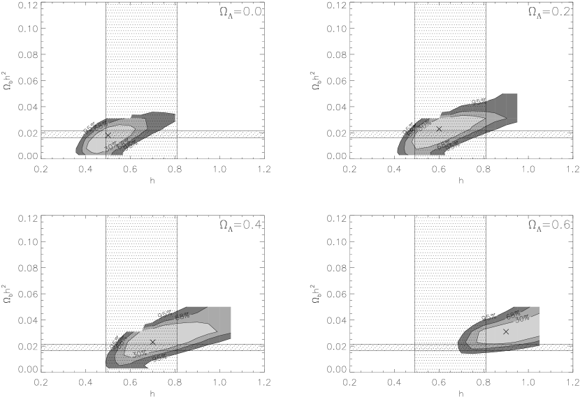
Figure 7: Goodness-of-fit contours for the joint fit to the CMB and APM data of a primordial spectrum with a ‘step’, for different choices of $\Omega_{\Lambda}$. The vertical and horizontal shaded bands indicate the constraints (4) and (5) on $h$ and $\Omega_{{\rm B}}h^{2}$ respectively while the crosses indicate the best fits from Table 3. Values of $\Omega_{\Lambda}\mathrel{\mathchoice{\lower 3.6pt\vbox{\halign{$\mathsurround=0pt\displaystyle\hfill#\hfil$\cr>\crcr\sim\crcr}}}{\lower 3.6pt\vbox{\halign{$\mathsurround=0pt\textstyle\hfill#\hfil$\cr>\crcr\sim\crcr}}}{\lower 3.6pt\vbox{\halign{$\mathsurround=0pt\scriptstyle\hfill#\hfil$\cr>\crcr\sim\crcr}}}{\lower 3.6pt\vbox{\halign{$\mathsurround=0pt\scriptscriptstyle\hfill#\hfil$\cr>\crcr\sim\crcr}}}}0.6$ provide an unacceptably poor fit to the data.

2.5 Implications for cluster abundances

In Table 4 we show also the value of the variance $\sigma(R)$ in (dark matter) fluctuations (normalised to the CMB), over a sphere of size $R=8\,h^{-1}{\rm Mpc}$:

$$\sigma^{2}(R)=\frac{1}{H_{0}^{4}}\int_{0}^{\infty}W^{2}(kR)~{}\delta_{\rm H}^{2}(k)~{}T^{2}(k)~{}k^{3}{\rm d}k,$$ (19)

using a ‘top hat’ smoothing function, $W(kR)=3[{\textstyle\frac{\sin(kR)}{(kR)^{3}}}-{\textstyle\frac{\cos(kR)}{(kR)^{2}}}]$. (The range of $\sigma_{8}$ for a given value of $\Omega_{\Lambda}$ corresponds to the range of the step-size $A/B$.) The tabulated values are systematically somewhat higher than the mean value $\sigma_{8}=0.56\Omega_{\rm m}^{-0.47}$ for flat cosmologies inferred from the observed abundances of X-ray emitting clusters, although within the 95% c.l. upper limit which is higher by $20\Omega_{\rm m}^{0.2\log\Omega_{\rm m}}$ per cent [Viana & Liddle 1999]. We wish to emphasise that the break in the primordial spectrum implies a much lower $\sigma_{8}$ than the corresponding H-Z spectrum with the same cosmological parameters. For example the COBE-normalised sCDM (H-Z) model with $\Omega_{m}\simeq 1$ gives $\sigma_{8}\simeq 1.4$ (e.g. Stompor, Gorski and Banday 1996) as opposed to $\sigma_{8}\simeq 0.65-0.73$ in Table 4, which is much closer to the value of $\sigma_{8}\simeq 0.56$ inferred from the cluster abundance. As shown in Figure 4, this is because of the decrease in power at small scales relative to a scale-invariant spectrum. Note that we cannot constrain well the region $k>0.2\,h\,{\rm Mpc}^{-1}$ (corresponding to $R<8\,h^{-1}{\rm Mpc}$), because of uncertainties in the reconstruction of the primordial spectrum due to non-linear biasing and non-linear gravity effects. For simplicity we have assumed a H-Z spectrum for $k>0.6\,h\,{\rm Mpc}^{-1}$ (Equation 12) so in principle other (smaller) values of $\sigma_{8}$ are also allowed. For instance, if there were further breaks in the primordial spectrum, as is quite possible, then a better agreement could easily be achieved. In order to constrain such possibilities we intend to investigate in further work the Lyman-$\alpha$ forest $P(k)$ and its evolution with redshift [Croft et al. 1999] which provides a probe of such small scales in the linear regime.

In Figure 8 we show the predictions for the redshift evolution of the cluster abundance in our models according to the Press-Schechter (P-S) theory [Press & Schechter 1974], compared to the observations as presented in Bahcall & Fan (1998). We consider clusters with mass $M>8\times 10^{14}M_{\odot}$ (neglecting the $R<R_{\rm com}=1.5\,h^{-1}{\rm Mpc}$ condition). The spatially flat COBE-normalised H-Z model with $\Omega_{\Lambda}=0.2$, $\Omega_{m}\simeq 0.8$ (top thick full line) does not match the observations, a fact that has been used to rule out this model. Even when this model is normalised at $z=0$ by lowering its amplitude to $\sigma_{8}\simeq 0.6$ (bottom thick full line), it still fails to reproduce the observed redshift evolution in the cluster abundances [Bahcall & Fan 1998]. By contrast, the best-fit models in Table 4 do match the redshift evolution, especially if we allow for the possibility mentioned above of lowering the $\sigma_{8}$ values further to better match the $z=0$ data. We emphasise that these predictions have not been adjusted in any way to fit cluster abundances; all parameters have been fixed already by the fit to the APM and CMB data. It is interesting to note that even the $\Omega_{\Lambda}=0$ model can now reproduce the slow growth of the cluster abundance with redshift due to the break in the primordial spectrum.

Figure 8: The number density of rich clusters with $M>8\times 10^{14}M_{\odot}$ as a function of redshift. Points with errorbars correspond to the observations as depicted in Bahcall & Fan (1998). The thick full lines correspond to the P-S prediction for the spatially flat, COBE-normalised H-Z model with $\Omega_{\Lambda}=0.2$, $\Omega_{m}\simeq 0.8$ (top line), and scaled to match the cluster abundance at $z=0$ (bottom line). The curves in between correspond to the best-fit models in Table 4 with $\Omega_{\Lambda}=0$ (full line), $\Omega_{\Lambda}=0.2$ (dashed line), $\Omega_{\Lambda}=0.4$ (dot-dashed line), and $\Omega_{\Lambda}=0.6$ (dotted line).

3 Discussion

Several authors have in the past noted the possibility of generating spectral features in the H-Z density perturbation by fine tuning the parameters of the inflaton potential [Kofman & Linde 1987, Salopek, Bond & Bardeen 1989, Hodges et al. 1990, Hodges & Blumenthal 1990]. We would like to emphasise that in contrast to such “designer” models, the break in the H-Z spectrum discussed here is generated by a physical mechanism, viz. supersymmetry breaking during inflation (Adams et al. 1997b, Ross 1998). As noted subsequently [Lesgourgues & Polarski 1997, Kanazawa et al. 2000], the resulting damping of the CMB anisotropy is also a characteristic of ‘double inflation’ which occurs in toy models wherein inflation is driven in two stages — first by higher-order gravity and then by a scalar field [Kofman, Linde & Starobinsky 1985, Kofman & Pogosyan 1988, Gottlöber, Müller & Starobinsky 1991], or by two coupled scalar fields [Starobinsky 1985, Kofman & Linde 1987, Polarski & Starobinsky 1992]. The model parameters can be tuned to generate a break in the primordial spectrum at any chosen scale. The advantages of this for fitting LSS observations was first emphasised by Silk & Turner (1987) and have been explored thoroughly [Polarski & Starobinsky 1992, Gottlöber, Mücket & Starobinsky 1994, Polarski 1994, Peter, Polarski & Starobinsky 1994, Amendola et al. 1995, Polarski & Starobinski 1995, Semig & Müller 1996], although these authors did not discuss the implications for the CMB. A spectral feature similar to that observed can also be generated in a toy model where the inflaton evolves through a kink in its potential [Starobinsky 1992], leading to similar suppression of the secondary acoustic peaks [Atrio-Barandela et al. 1997, Lesgourgues, Polarski & Starobinsky 1998, Lesgourgues, Prunet & Polarski 1999]. Recently there have been efforts to progress beyond toy models and implement multiple inflation in supersymmetric models [Sakellariadou & Tetradis 1998, Lesgourgues 1998, Lesgourgues 2000]. Spectral features can also be generated by resonant production of particles during inflation [Chung et al. 2000].

Silk & Gawiser (2000) have noted independently that it is difficult for a $\Lambda$CDM model to fit LSS and CMB observations simultaneously without considering departures from scale-invariance; they advocate adding a ‘bump’ at $k\sim 0.06\,h\,{\rm Mpc}^{-1}$ to a primordial H-Z spectrum. Einasto et al. (1999) have also concluded from an exhaustive analysis of LSS data that a scale-free primordial spectrum is excluded. In particular it has been noted that the power spectrum of clusters is better fitted if the primordial spectrum has a step-like feature at $k\sim 0.1\,h\,{\rm Mpc}^{-1}$ [Gramann & Suhhonenko 1999]. The implications of broken scale-invariance for accurate determination of cosmological parameters using forthcoming LSS and CMB data have been investigated [Wang, Spergel & Strauss 1999, Hannestad 2000].

It is clear that the notion of a scale imprinted on the primordial density perturbation is favoured by a number of observational considerations as well as having a natural physical interpretation in the context of realistic inflationary models. In this paper we have demonstrated that the recent small angular-scale CMB anisotropy data favour a deviation from scale-invariance in the range $k\sim(0.06-0.6)h\,{\rm Mpc}^{-1}$ independently of the similar previous indication from studies of LSS, in particular the APM survey. This is reassuring since the latter rests on the assumption (for which arguments are given in Appendix A) that there is no scale-dependent bias between APM galaxies and dark matter.

Allowing the primordial spectrum to depart from scale-invariance has important consequences for the deductions that can be made about cosmological parameters from LSS and CMB data. The standard interpretation of LSS data (e.g. APM $P(k)$ and $\sigma_{8}$ from cluster abundances) favours a low $\Gamma\sim\Omega_{m}{h}\sim 0.2$ universe assuming a COBE-normalised H-Z spectrum. However as we have shown these observations can be satisfactorily accounted for with much larger values of $\Omega_{m}$ if we allow for a break in the primordial spectrum. Our best fit models in Table 4, which obey the BBN constraint (5) on the baryon density, prefer higher values of $\Omega_{m}$ (and lower values of $\Omega_{\Lambda}$). The required amplitude of the break decreases with increasing $\Omega_{\Lambda}$ but one cannot do without such a break altogether. In particular the value $\Omega_{\Lambda}\sim 0.7$ favoured by the SN Ia data [Perlmutter et al. 1999, Riess et al. 1998] is not permitted, while it is quite possible to have a universe with zero cosmological constant and $\Omega_{m}=1$. Of course the high observed fraction of baryons in clusters, combined with the BBN value of the baryon density (5), implies an independent limit on the matter density [White et al. 1993]; a recent analysis quotes $\Omega_{\rm m}<0.31\,h^{-1/2}$ at 95% c.l. [Mohr, Haiman & Holder 2000]. There are many assumptions made in such analyses, viz. that clusters are spherical and in hydrostatic equilibrium with an isothermal temperature profile, that the measured baryon fraction reflects the universal value, that there is no preheating before or energy injection after cluster formation, etc. It is important to reassess these issues in the light of our increasing understanding of galaxy and cluster formation to quantify the systematic uncertainties better.

The hypothesis of a primordial density perturbation with broken scale-invariance, although radical, is eminently falsifiable. The ongoing 2DF and SDSS redshift surveys can confirm or rule out such a feature in the power spectrum of galaxy clustering, while the forthcoming MAP and Planck missions will determine whether all the secondary acoustic peaks in the CMB angular spectrum are indeed suppressed as expected. By contrast the alternative hypothesis of a baryon density $\sim 65\%$ higher than the BBN value predicts a boosted third peak (e.g. Tegmark & Zaldariagga 2000), so this would be a definitive test distinguishing between the two possibilities. We note that in either case there are important implications for the physics of the early universe. To increase the baryon-to-photon ratio after BBN by $\sim 65\%$ requires a decrease in the comoving entropy; the only mechanism suggested which can achieve this proposes that the photons in our universe become cooled through their coupling to a ‘shadow’ universe [Bartlett & Hall 1991]. However this possibility, recently invoked by Kaplinghat and Turner (2000), was shown to be severely constrained, if not ruled out altogether, from considerations of the concommitant spectral distortion in the CMB together with the bound from Supernova 1987a on new weakly interacting particles [Birkel & Sarkar 1997]. By contrast broken scale-invariance has a natural explanation in a phase transition occuring during inflation as expected in supersymmetric theories. If established this would provide the first direct connection between astronomical data and physics at very high energies.

Appendix A The effects of biasing

Independently of how or where galaxies form they must eventually fall into the dominant gravitational wells and thus trace out the underlying mass distribution (see Peebles 1980, Fry 1996). However, in principle, the galaxy distribution may be ‘biased’ with respect to the underlying mass fluctuations (e.g. Bardeen et al. 1986). There are several observations indicating that this effect is in fact small. The theoretical predictions for the first few connected moments, based on this hypothesis [Juszkiewicz, Bouchet & Colombi 1993, Bernardeau 1994a, Bernardeau 19994b] are in good agreement with the APM data [Gaztañaga 1994, Gaztañaga & Frieman 1994, Frieman & Gaztañaga 1999]. The current precision of this higher order correlation test is 20% and expected to improve with further data. The APM angular correlation function $\xi_{g}(r)$ shows an inflection point near $\xi_{g}\simeq 1$ very similar to the long awaited ‘shoulder’ in $\xi\simeq 1$, generated by gravitational dynamics [Gott & Rees 1975]. The agreement between the two characteristic scales can be used to constrain the linear biasing factor for the APM catalogue to be within 20% of unity [Gaztañaga & Juszkiewicz 2000]. We summarise these arguments [Gaztañaga & Baugh 1998] below for completeness since the assumption of small or no bias is crucial for the present study.

Let us assume that the (smoothed) galaxy fluctuations $\delta_{g}$ are related to those in the mass $\delta_{m}$ by a local transformation, $\delta_{g}(x)=F[\delta_{m}(x)]$, which can be expanded as a Taylor series: $F=b_{1}\delta_{m}+b_{2}\delta_{m}^{2}+\ldots$. Then the 2-point function $\xi_{2}^{g}(r)\equiv\langle\delta_{g}(x)\delta_{g}(x+r)\rangle$ on the scale $r$ will be:

$$\xi_{2}^{g}(r) = b_{1}^{2}\xi_{2}^{m}(r)+b_{1}b_{2}\langle\delta_{m}(x)\delta_{m}(x+r)^{2}\rangle$$ (20)

$$+b_{1}b_{2}\langle\delta_{m}^{2}(x)\delta_{m}(x+r)\rangle+\ldots,$$

where all further terms are of order 4 or higher in $\delta_{m}$ and correspond therefore to either higher order correlations, $\xi_{J}$ with $J>2$, or higher powers in $\xi_{2}$. If $\delta_{m}$ is Gaussian or hierarchical (as is the case for evolution through gravity), the higher order correlations $\xi_{J}$ are at most of order $\xi_{2}^{J-1}$. This means that at large scales where $\xi_{2}<1$, the first term is dominant so that only the amplitude of the 2-point statistics, but not its shape, may be altered by biasing. This has been confirmed in N-body simulations and galaxy biasing models [Mo, Jing & White 1997, Scoccimarro et al 2000].

Figure 9: The ratio of the non-linear to linear power spectrum illustrating non-linear effects on $P(k)$. Long and short-dashed lines show non-linear effects in the mass while the other lines show non-linear effects in the final galaxy distribution for various halo models (from Scoccimarro et al 2000).

Thus from the above arguments, the small variance on large scales ($R\mathrel{\mathchoice{\lower 3.6pt\vbox{\halign{$\mathsurround=0pt\displaystyle\hfill#\hfil$\cr>\crcr\sim\crcr}}}{\lower 3.6pt\vbox{\halign{$\mathsurround=0pt\textstyle\hfill#\hfil$\cr>\crcr\sim\crcr}}}{\lower 3.6pt\vbox{\halign{$\mathsurround=0pt\scriptstyle\hfill#\hfil$\cr>\crcr\sim\crcr}}}{\lower 3.6pt\vbox{\halign{$\mathsurround=0pt\scriptscriptstyle\hfill#\hfil$\cr>\crcr\sim\crcr}}}}8\,h^{-1}{\rm Mpc}$) means that it is reasonable to assume that the shape of $P(k)$ for galaxies at scales $k\mathrel{\mathchoice{\lower 3.6pt\vbox{\halign{$\mathsurround=0pt\displaystyle\hfill#\hfil$\cr<\crcr\sim\crcr}}}{\lower 3.6pt\vbox{\halign{$\mathsurround=0pt\textstyle\hfill#\hfil$\cr<\crcr\sim\crcr}}}{\lower 3.6pt\vbox{\halign{$\mathsurround=0pt\scriptstyle\hfill#\hfil$\cr<\crcr\sim\crcr}}}{\lower 3.6pt\vbox{\halign{$\mathsurround=0pt\scriptscriptstyle\hfill#\hfil$\cr<\crcr\sim\crcr}}}}0.1\,h\,{\rm Mpc}^{-1}$ coincides with the shape of the underlying linear matter power spectrum. This argument, which is based simply on the smallness of the variance and the assumption of hierarchical clustering, can also be applied to gravity, since the leading contribution to the correlation functions in perturbation theory is indeed given by a local transformation (see Fosalba & Gaztañaga 1997). This is clearly illustrated in Figure 11 of Gaztañaga and Baugh (1998). By comparing the linear and non-linear shape of $P(k)$, one can see that it has not been changed significantly through gravitational evolution on scales where the rms fluctuations are small, i.e. for $k\mathrel{\mathchoice{\lower 3.6pt\vbox{\halign{$\mathsurround=0pt\displaystyle\hfill#\hfil$\cr<\crcr\sim\crcr}}}{\lower 3.6pt\vbox{\halign{$\mathsurround=0pt\textstyle\hfill#\hfil$\cr<\crcr\sim\crcr}}}{\lower 3.6pt\vbox{\halign{$\mathsurround=0pt\scriptstyle\hfill#\hfil$\cr<\crcr\sim\crcr}}}{\lower 3.6pt\vbox{\halign{$\mathsurround=0pt\scriptscriptstyle\hfill#\hfil$\cr<\crcr\sim\crcr}}}}0.1\,h\,{\rm Mpc}^{-1}$.

How important are non-linearities for $\delta\mathrel{\mathchoice{\lower 3.6pt\vbox{\halign{$\mathsurround=0pt\displaystyle\hfill#\hfil$\cr>\crcr\sim\crcr}}}{\lower 3.6pt\vbox{\halign{$\mathsurround=0pt\textstyle\hfill#\hfil$\cr>\crcr\sim\crcr}}}{\lower 3.6pt\vbox{\halign{$\mathsurround=0pt\scriptstyle\hfill#\hfil$\cr>\crcr\sim\crcr}}}{\lower 3.6pt\vbox{\halign{$\mathsurround=0pt\scriptscriptstyle\hfill#\hfil$\cr>\crcr\sim\crcr}}}}1$, i.e. for $k\mathrel{\mathchoice{\lower 3.6pt\vbox{\halign{$\mathsurround=0pt\displaystyle\hfill#\hfil$\cr>\crcr\sim\crcr}}}{\lower 3.6pt\vbox{\halign{$\mathsurround=0pt\textstyle\hfill#\hfil$\cr>\crcr\sim\crcr}}}{\lower 3.6pt\vbox{\halign{$\mathsurround=0pt\scriptstyle\hfill#\hfil$\cr>\crcr\sim\crcr}}}{\lower 3.6pt\vbox{\halign{$\mathsurround=0pt\scriptscriptstyle\hfill#\hfil$\cr>\crcr\sim\crcr}}}}0.1\,h\,{\rm Mpc}^{-1}$? Figure 9 shows the ratio of the non-linear to linear power spectrum $P(k)$, normalised to be unity at small $k$ in order to emphasize the non-linear effects. The long-dashed line corresponds to the APM-like $P(k)$ for $\Omega=1$ dynamics (from N-body simulations in Baugh & Gaztañaga 1996). The short-dashed line corresponds to a $\Omega=0.3$, $\Lambda=0.7$ $\Lambda$CDM model (using the non-linear mass fitting formulae). The dotted, continuous and dot-dashed lines correspond to different non-linear models for galaxy formation based on halo models (with linear bias $b\mathrel{\mathchoice{\lower 3.6pt\vbox{\halign{$\mathsurround=0pt\displaystyle\hfill#\hfil$\cr<\crcr\sim\crcr}}}{\lower 3.6pt\vbox{\halign{$\mathsurround=0pt\textstyle\hfill#\hfil$\cr<\crcr\sim\crcr}}}{\lower 3.6pt\vbox{\halign{$\mathsurround=0pt\scriptstyle\hfill#\hfil$\cr<\crcr\sim\crcr}}}{\lower 3.6pt\vbox{\halign{$\mathsurround=0pt\scriptscriptstyle\hfill#\hfil$\cr<\crcr\sim\crcr}}}}1.5$ for $\sigma_{8}\simeq 1$) from Figure 6 in Scoccimarro et al (2000). In all cases non-linear effects become significant ($>10\%$) only at $k\mathrel{\mathchoice{\lower 3.6pt\vbox{\halign{$\mathsurround=0pt\displaystyle\hfill#\hfil$\cr>\crcr\sim\crcr}}}{\lower 3.6pt\vbox{\halign{$\mathsurround=0pt\textstyle\hfill#\hfil$\cr>\crcr\sim\crcr}}}{\lower 3.6pt\vbox{\halign{$\mathsurround=0pt\scriptstyle\hfill#\hfil$\cr>\crcr\sim\crcr}}}{\lower 3.6pt\vbox{\halign{$\mathsurround=0pt\scriptscriptstyle\hfill#\hfil$\cr>\crcr\sim\crcr}}}}0.2\,h\,{\rm Mpc}^{-1}$ and are of order unity by $k\sim 1\,h\,{\rm Mpc}^{-1}$. Non-linear effects seem smaller for galaxies than for the dark matter (in agreement with the observed $S_{J}$ in Baugh & Gaztañaga 1996). One could imagine constructing galaxy formation models with stronger non-linear effects, but it will then be difficult to account for the observed galaxy higher-order correlations. As pointed out in Scoccimarro et al (2000), galaxy clustering in the framework of the halo models is strongly constrained by the measured galaxy skewness. Thus, given current observational constraints and present understanding of galaxy formation one can conclude that non-linear effects cannot have altered the linear $P(k)$ by a factor exceeding $\sim 2$, up to $k\simeq 1\,h\,{\rm Mpc}^{-1}$ .

References

- [Adams, Ross & Sarkar 1997a] Adams J.A., Ross G.G., Sarkar S., 1997a, Phys. Lett., B391, 271
- [Adams, Ross & Sarkar 1997b] Adams J.A., Ross G.G., Sarkar S., 1997b, Nucl. Phys., B503, 405
- [Amendola et al. 1995] Amendola L., Gottlöber S., Mücket J.P., Müller V., 1995, ApJ, 451, 444
- [Atrio-Barandela et al. 1997] Atrio-Barandela F., Einasto J., Gottlöber S., Müller V., Starobinsky A.A., 1997, JETP Lett., 66, 397
- [Bahcall et al. 1999] Bahcall N., Ostriker J.P., Perlmutter S., Steinhardt P., Science, 1999, 284, 1481
- [Bahcall & Fan 1998] Bahcall N., Fan X., 1998, ApJ, 504, 1
- [Balbi et al. 2000] Balbi A. et al. (MAXIMA collab.), 2000, ApJ, 545, L1
- [Bardeen et al. 1986] Bardeen J.M., Bond J.R., Kaiser N., Szalay A.S., 1986, ApJ, 321, 28
- [Bardeen, Steinhardt & Turner 1983] Bardeen J.M., Steinhardt P.J., Turner M.S., 1983, Phys. Rev., D28, 697
- [Barreiro et al. 1996] Barreiro T., Copeland E.J., Lyth D.H., Prokopec T., 1996, Phys. Rev., D54, 1379
- [Bartlett et al. 1995] Bartlett J.G., Blanchard A., Silk J., Turner M.S., 1995, Science, 267, 980
- [Bartlett & Hall 1991] Bartlett J.G., Hall L.J., 1991, Phys. Rev. Lett., 66, 541
- [Baugh & Efstathiou 1993] Baugh C.M., Efstathiou G.P., 1993, MNRAS, 265, 145
- [Baugh & Gaztañaga 1996] Baugh C.M., Gaztañaga E., 1996, MNRAS, 280, L37
- [Bennett et al. 1996] Bennett C.L. et al. (COBE collab.), 1996, ApJ, 464, L1
- [Bernardeau 1994a] Bernardeau F., 1994a, A&A, 291, 697
- [Bernardeau 19994b] Bernardeau F., 1994b, ApJ, 433, 1
- [Bertschinger 1995] Bertschinger E., preprint (astro-ph/9506070)
- [Birkel & Sarkar 1997] Birkel M., Sarkar S., 1997, Phys. Lett. B408, 59
- [Bond & Efstathiou 1984] Bond J.R., Efstathiou G., 1984, ApJ, 285, L45
- [Bond & Jaffe 1999] Bond J.R., Jaffe A.H., 1999, Phil. Trans. R. Soc. Lond., 357, 57
- [Bonifacio & Molaro 1997] Bonifacio P., Molaro P., 1997, MNRAS, 285, 847
- [Bunn & White 1997] Bunn E.F., White M., 1997, ApJ, 480, 6
- [Burles, Kirkman & Tytler 1999] Burles S., Kirkman D., Tytler D., 1999, ApJ 519, 18
- [Burles et al. 1999] Burles S., Nollett K.M., Truran J.N., Turner M.S., 1999, Phys. Rev. Lett., 82, 4176
- [Burles & Tytler 1998] Burles S., Tytler D., 1998, ApJ, 507, 732
- [Chung et al. 2000] Chung D., Kolb E.W., Riotto A., Tkachev I.I., 2000, Phys. Rev. D62, 043508
- [Coughlan et al. 1984] Coughlan G., Fischler W., Kolb E.W., Raby S., Ross G.G., 1984, Phys. Lett., 140B, 44
- [Covi & Lyth 2000] Covi L., Lyth D., 2000, MNRAS, to appear (astro-ph/0008165)
- [de Bernadis et al. 2000] de Bernadis P. et al. (Boomerang collab.), 2000, Nat, 404, 955
- [Croft et al. 1999] Croft R., Weinberg D.H., Pettini M., Hernquist L., Katz N., 1999, ApJ, 520, 1
- [Dine et al. 1984] Dine M., Fischler W., Nemechansky D., 1984, Phys. Lett., 136B, 169
- [Efstathiou, Bond & White 1992] Efstathiou G., Bond J.R., White S.D.M., 1992, MNRAS, 258, 1P
- [Einasto et al. 1999] Einasto J. et al., 1999, ApJ, 519, 469
- [Eke et al. 1998] Eke V.R., Cole S., Frenk C.S., Henry P.J., 1998, MNRAS, 298, 1145
- [Esposito et al. 2001] Esposito S., Mangano G., Melchiorri A., Miele G., Pisanti O., 2001, Phys. Rev., D63, 043004
- [Fiorentini et al. 1998] Fiorentini G., Lisi E., Sarkar S., Villante F., 1998, Phys. Rev., D58, 063506
- [Fosalba & Gaztañaga 1997] Fosalba P., Gaztañaga E., 1997, MNRAS, 301, 535
- [Frieman & Gaztañaga 1999] Frieman J.A., Gaztañaga E., 1999, ApJ, 521, L83
- [Fry 1996] Fry, J. 1996, ApJ, 461, L65
- [Fukugita, Hogan & Peebles 1998] Fukugita M., Hogan C., Peebles P.J.E., 1998, ApJ, 503, 518
- [Gaztañaga 1994] Gaztañaga E., 1994, MNRAS, 268, 913
- [Gaztañaga & Baugh 1998] Gaztañaga E., Baugh C.M., 1998, MNRAS, 294, 229
- [Gaztañaga & Frieman 1994] Gaztañaga E., Frieman J.A., 1994, ApJ, 437, L13
- [Gaztañaga & Juszkiewicz 2000] Gaztañaga E., Juszkiewicz R., preprint (astro-ph/0007087)
- [Gott & Rees 1975] Gott J.R., Rees M.J., 1975, A&A, 45, 365
- [Gottlöber, Müller & Starobinsky 1991] Gottlöber S., Müller V., Starobinsky A.A., 1991, Phys. Rev., D43, 2510
- [Gottlöber, Mücket & Starobinsky 1994] Gottlöber S., Mücket J.P., Starobinsky A.A., 1994, ApJ, 434, 417
- [Gramann & Suhhonenko 1999] Gramann M., Suhhonenko I., ApJ, 519, 433
- [Griffiths, Silk & Zaroubi 2000] Griffiths L., Silk J., Zaroubi S., 2000, preprint (astro-ph/0010571)
- [Guth & Pi 1982] Guth A.H., S.-Y. Pi, 1982, Phys. Rev. Lett., 49, 1110
- [Hamilton & Tegmark 2000] Hamilton A., Tegmark M., 2000, preprint (astro-ph/0008392)
- [Hanany et al. 2000] Hanany S. et al. (MAXIMA collab.), 2000, ApJ, 545, L5
- [Hannestad 2000] Hannestad S., 2000, Phys. Rev. D, to appear (astro-ph/0009296)
- [Hawking 1982] Hawking S.W., 1982, Phys. Lett., 115B, 295
- [Hodges & Blumenthal 1990] Hodges H., Blumenthal G.R., 1990, Phys. Rev., D42, 3329
- [Hodges et al. 1990] Hodges H., Blumenthal G.R., Kofman L.A., Primack J.R., 1990, Nucl. Phys. B335, 197
- [Hu et al. 2000] Hu W., Fukugita M., Zaldarriaga M., Tegmark M., 2000, ApJ, to appear (astro-ph/0006436)
- [Izotov, Thuan & Lipovetsky 1998] Izotov Y.I., Thuan T.X., Lipovetsky V.A., 1998, ApJ, 500, 188
- [Izotov et al. 2000] Izotov Y.I., Chafee F.H., Foltz C.B., Green R.F., Guseva N.G., Thuan T.X., 2000, ApJ, 527, 757
- [Jaffe et al. 2000] Jaffe A.H. et al., 2000, Phys. Rev. Lett., in press (astro-ph/0007333)
- [Jain, Mo & White 1995] Jain B., Mo H.J., White S.D.M., 1995, MNRAS, 276, L25.
- [Juszkiewicz, Bouchet & Colombi 1993] Juszkiewicz R., Bouchet F., Colombi S., 1993, ApJ, 412, L9
- [Kanazawa et al. 2000] Kanazawa T., Kawasaki M., Sugiyama N., Yanagida T., 2000, Phys. Rev., D61, 023517
- [Kaplinghat & Turner 2000] Kaplinghat M., Turner M.S., 2000, Phys. Rev. Lett., 86, 385
- [Kernan & Sarkar 1996] Kernan P., Sarkar S., 1996, Phys. Rev. D54, 3681
- [Kinney, Melchiorri & Riotto 2000] Kinney W.H., Melchiorri A., Riotto A., 2000, Phys. Rev. D63, 023505
- [Kirkman et al. 2000] Kirkman D., Tytler D., Burles S., Lubin D., O’Meara J.M., 2000, ApJ, 529, 655
- [Kofman & Linde 1987] Kofman L.A., Linde A.D., 1987, Nucl. Phys., B282, 555
- [Kofman, Linde & Starobinsky 1985] Kofman L.A., Linde A.D., Starobinsky A.A., 1985, Phys. Lett., B157, 361
- [Kofman & Pogosyan 1988] Kofman L.A., Pogosyan D., 1988, Phys. Lett., B214, 508
- [Krauss 2000] Krauss L.M., 2000, Phys. Rep., 333-334, 33
- [Lange et al. 2001] Lange A.E. et al. (Boomerang collab.), 2001, Phys. Rev. D63, 042001
- [Lesgourgues 1998] Lesgourgues J., 1998, Phys. Lett., B452, 15
- [Lesgourgues 2000] Lesgourgues J., 2000, Nucl. Phys., B582, 593
- [Lesgourgues & Polarski 1997] Lesgourgues J., Polarski D., 1997, Phys. Rev., D56, 6425
- [Lesgourgues, Polarski & Starobinsky 1998] Lesgourgues J., Polarski D., Starobinsky A.A., 1998, MNRAS, 297, 769
- [Lesgourgues, Prunet & Polarski 1999] Lesgourgues J., Prunet S., Polarski D.,1999, MNRAS, 303, 45
- [Levshakov, Kegel & Takahara 1999] Levshakov S.A., Kegel W.H., Takahara F., 1999, MNRAS, 302, 707
- [Lineweaver & Barbosa 1998] Lineweaver C., Barbosa D., 1998, A&A, 329, 799
- [Lyth & Riotto 1999] Lyth D., Riotto A., 1999, Phys. Rep., 314, 1
- [Lyth & Stewart 1996] Lyth D., Stewart E.D., 1996, Phys. Rev., D53, 1784
- [Maddox et al. 1990a] Maddox S.J., Efstathiou G.,Sutherland W.J., Loveday J., 1990a, MNRAS 242, 43P
- [Maddox et al. 1990b] Maddox S.J., Efstathiou G.,Sutherland W.J., Loveday J., 1990b, MNRAS 243, 692
- [McCullough 1992] McCullough P.R., 1992, ApJ, 390, 213
- [Mo, Jing & White 1997] Mo H.J., Jing Y.P., White S.D.M., 1997, MNRAS, 282, 1096
- [Mohr, Haiman & Holder 2000] Mohr J.J., Haiman Z., Holder G.P., 2000, preprint (astro-ph/0004244)
- [Mould et al. 2000] Mould J.R. et al., 2000, ApJ, 529, 786
- [Mukhanov & Chibisov 1981] Mukhanov V.F. & Chibisov G.V., 1981, JETP Lett., 33, 532
- [Olive, Skillman & Steigman 1997] Olive K.A., Skillman E., Steigman G., 1997, ApJ, 483, 788
- [Padmanabhan & Sethi 2000] Padmanabhan T. and Sethi S.K., 2000, preprint (astro-ph/0010309)
- [Parodi et al. 2000] Parodi B.R., Saha A., Tammann G.A., Sandage A., 2000, ApJ, 540, 634
- [Peacock 1997] Peacock J.A., 1997, MNRAS, 284, 885.
- [Peacock & Dodds 1994] Peacock J.A., Dodds S.J., 1994, MNRAS, 267, 1020
- [Peacock & Dodds 1996] Peacock J.A., Dodds S.J., 1996, MNRAS, 280, L19
- [Peebles 1980] Peebles P.J.E., 1980, The Large–Scale Structure of the Universe, Princeton University Press, Princeton
- [Peimbert, Peimbert & Ruiz 2000] Peimbert M., Peimbert A., Ruiz M.T., 2000, ApJ, 541, 688
- [Perlmutter et al. 1999] Perlmutter S. et al., 1999, ApJ, 517, 565
- [Peter, Polarski & Starobinsky 1994] Peter P., Polarski D., Starobinsky A.A., 1994, Phys. Rev., D50, 4827
- [Polarski 1994] Polarski D., 1994, Phys. Rev., D49, 6319
- [Polarski & Starobinsky 1992] Polarski D., Starobinsky A.A., 1992, Nucl. Phys., B385, 623
- [Polarski & Starobinski 1995] Polarski D., Starobinsky A.A., 1995, Phys. Lett., B356, 196
- [Press & Schechter 1974] Press W.H., Schechter P., 1974, ApJ 187, 425
- [Primack 2000] Primack J., 2000, preprint (astro-ph/0007187)
- [Riess et al. 1998] Riess A.G. et al., 1998, AJ, 116, 1009
- [Ross 1998] Ross G.G., 1998, in Roszkowski L., ed., Proc. COSMO 97, World Scientific, Singapore, p.333
- [Sakellariadou & Tetradis 1998] Sakellariadou M., Tetradis N., 1998, hep-ph/9806461
- [Salopek, Bond & Bardeen 1989] Salopek D.S., Bond J.R., Bardeen J.M., 1989, Phys. Rev. D40, 1753
- [Scoccimarro et al 2000] Scoccimarro R., Sheth R., Hui L., Jain B., 2000, preprint (astro-ph/0006319)
- [Seljak & Zaldarriaga 1996] Seljak U, Zaldariagga M., 1996, ApJ, 469, 437
- [Semig & Müller 1996] Semig L.V., Müller V., 1996, A&A, 308, 697
- [Silk & Gawiser 1998] Silk J., Gawiser E., 2000, Phys. Scr., T85, 132
- [Silk & Turner 1987] Silk J, Turner M.S., 1987, Phys. Rev., D35, 419
- [Smoot et al. 1992] Smoot G.F. et al. (COBE collab.), 1992, ApJ, 396, L1
- [Songaila et al. 1994] Songaila A., Cowie L.L., Hogan C.J., Rugers M., 1994, Nature, 368, 599
- [Starobinsky 1982] Starobinsky A.A., Phys. Lett., 1982, 117B, 175
- [Starobinsky 1985] Starobinsky A.A., JETP Lett., 1985, 42, 152
- [Starobinsky 1992] Starobinsky A.A., JETP Lett., 1992, 55, 489
- [Stompor, Gorski & Banday 1996] Stompor R., Gorski K.M., Banday A.J., 1996, MNRAS, 277, 1225
- [Tegmark & Hamilton 1997] Tegmark M., Hamilton A.J.S., 1997, preprint (astro-ph/9702019)
- [Tegmark, Zaldarriaga & Hamilton2001] Tegmark M., Zaldarriaga M., Hamilton A.J.S. 2001, Phys. Rev., D63, 043007
- [Tegmark & Zaldarriaga 2000] Tegmark M., Zaldarriaga M., 2000, Phys. Rev. Lett., 85, 2240
- [Theuns et al. 1999] Theuns T., Leonard A., Schaye J., Efstathiou G., 1999, MNRAS, 303, L58
- [Tonry et al. 2000] Tonry J.L., Blakeslee J.P., Ajhar E.A., Dressler A., 2000, ApJ, 530, 625
- [Wang, Spergel & Strauss 1999] Wang Y., Spergel D., Strauss M.A., 1999, ApJ, 510, 20
- [Tytler et al. 1999] Tytler D., Burles S., Lu L., Fan X-M., Wolfe A., Savage B.D., AJ, 117, 63
- [Vauclair & Charbonnel 1998] Vauclair S., Charbonnel C., 1998, ApJ, 502, 372
- [Viana & Liddle 1999] Viana P., Liddle A.R., 1999, MNRAS, 303, 535
- [Vittorio & Silk 1992] Vittorio N., Silk J, 1992, ApJ, 385, L9
- [Weinberg et al. 1997] Weinberg D.H., Miralda-Escudé J., Hernquist L., Katz N., 1997, ApJ, 490, 564
- [Weinberg et al. 1999] Weinberg D.H., Croft R., Hernquist L., Katz N., Pettini M., 1999, ApJ, 522, 563
- [White et al. 1995] White M., Scott D., Silk J., Davis M., 1995, MNRAS, 276, L69
- [White et al. 1995] White M., Viana P.T.P., Liddle A.R., Scott D., 1996, MNRAS, 283, 107
- [White et al. 1993] White S.D.M., Navarro J.F., Evrard A.E., Frenk C.S., 1993, Nature, 366, 429
- [Yamamoto 1986] Yamamoto K., 1986, Phys. Lett., 168B, 341