A Measurement of the Three–Dimensional Clustering
of C IV Absorption–Line Systems on Scales of 5 to 300 $h^{-1}$ Mpc

Abstract

We examine the three–dimensional clustering of C IV absorption–line systems, using an extensive catalog of QSO heavy–element absorbers drawn from the literature. We measure clustering by a volume–weighted integral of the correlation function called the reduced second–moment measure, and include information from both along and across QSO lines of sight, thus enabling a full determination of the three–dimensional clustering of absorbers, as well as a comparison of line– and cross–line–of–sight clustering properties. Here we present the three–dimensional reduced second–moment estimator for a three–dimensional point process probed by one–dimensional lines of sight, and apply our algorithm to a sample of 345 C IV absorbers with median redshift $\langle z\rangle=2.2$, drawn from the spectra of 276 QSOs. We confirm the existence of significant clustering on comoving scales up to 100 $h^{-1}$ Mpc ($q_{0}=0.5$), and find that the additional cross–line–of–sight information strengthens the evidence for clustering on scales from 100 $h^{-1}$ Mpc to 150 $h^{-1}$ Mpc. There is no evidence of absorber clustering along or across lines of sight for scales from 150 $h^{-1}$ Mpc to 300 $h^{-1}$ Mpc. We show that with a 300–times larger catalog, such as that to be compiled by the Sloan Digital Sky Survey (100,000 QSOs), use of the full three–dimensional estimator and cross–line–of–sight information will substantially increase clustering sensitivity. We find that standard errors are reduced by a factor 2 to 20 on scales of 30 to 200 $h^{-1}$ Mpc, in addition to the factor of $\sqrt{300}$ reduction from the larger sample size, effectively increasing the sample size by an extra factor of 4 to 400 at large distances.

1 Introduction

In a previous series of investigations (Vanden Berk et al., 1996; Quashnock, Vanden Berk, & York, 1996; Quashnock & Vanden Berk, 1998), the clustering properties of C IV and Mg II absorbers have been investigated, using an extensive catalog of heavy–element absorption–line systems drawn from the literature. These authors used a one–dimensional correlation analysis — one confined to pairs of absorbers along the same QSO line of sight — and found evidence for strong and evolving clustering on small scales (1–16 $h^{-1}$ Mpc), as well as for superclustering on scales as large as 50–100 $h^{-1}$ Mpc. Together, these investigations suggest that these strong absorbers, with median rest equivalent width $\langle W\rangle=0.4$ Å for C IV (Quashnock & Vanden Berk, 1998), are biased tracers of the higher density regions of space, and that agglomerations of absorbers along a line of sight are indicators of clusters and superclusters.

Recently, Quashnock & Stein (1999) used a new measure of clustering, called the reduced second moment measure or $K(r)$ (Ripley, 1988; Baddeley, 1998), which directly measures the mean overdensity of absorbers on scales $\mathrel{\hbox{\hbox to0.0pt{\hbox{\lower 4.0pt\hbox{$\sim$}}\hss}\hbox{$<$}}}r$. While closely related to other second–order measures of clustering, such as the correlation function or the power spectrum, the reduced second moment measure nevertheless has a number of advantageous statistical properties, and has recently been studied by astrophysicists (Martínez et al., 1998; Quashnock & Stein, 1999; Stein, Quashnock, & Loh, 2000). Quashnock & Stein (1999) found significant evidence for clustering of C IV absorbers on scales of 20–100 $h^{-1}$ Mpc, with marginal evidence on 100–200 $h^{-1}$ Mpc scales, again suggesting that the absorbers show superclustering much like what is seen locally in the distribution of galaxies.

However, their analysis also was confined to pairs of absorbers along the same line of sight, and hence did not include cross–line–of–sight information valuable for a full determination of the three–dimensional clustering properties of absorbers, which we are ultimately interested in finding. Indeed, Richards et al. (1999) have claimed that there is evidence of some significant contamination of true intervening systems along the line of sight by absorbers that are actually physically associated with the QSO, and that such contamination may extend to relative velocities as great as 75000 km s^-1. This means that such a contamination could be present as well in the superclustering signal found by Quashnock & Stein (1999). In addition, on smaller scales of a few megaparsecs, Crotts, Burles, & Tytler (1997) have claimed that the clustering of C IV systems across adjacent lines of sight is significantly weaker than along a line of sight and have questioned whether the correlations are due to velocity dispersion in associated systems rather than intrinsic spatial clustering. The number of adjacent lines analyzed by Crotts, Burles, & Tytler (1997) was small, however.

It is thus essential to study correlations both along and across QSO lines of sight, to enable a complete determination of the three–dimensional clustering of absorbers, as well as a comparison of line– and cross–line–of–sight clustering properties (and ultimately statistically discriminate between intrinsic and intervening absorbers). What is required is a method that measures spatial clustering of absorbers — which are nonetheless confined to QSO lines of sight — and can contrast clustering along and across lines of sight.

Here we present the three–dimensional estimator for the reduced second moment measure of a three–dimensional point process probed by one–dimensional lines of sight. We apply our algorithm to a sample of 345 C IV absorbers with median redshift $\langle z\rangle=2.2$, drawn from the spectra of 276 QSOs in the aforementioned catalog of Vanden Berk et al., with the goal of determining the clustering of absorbers on very large scales and seeing if the signal found by Quashnock & Stein (1999) remains when including cross–line–of–sight information, or, more compellingly, using only cross–line–of–sight information.

The outline of the paper is as follows: In §2 we define the three–dimensional reduced second moment measure, compare it to its one–dimensional analog, and outline our method of estimation. In §3 we apply our methodology to the above sample and present our results. In §4 we interpret the results and discuss how the full three–dimensional estimator and cross–line–of–sight information will improve our ability to measure clustering with the absorber sample from the Sloan Digital Sky Survey (100,000 QSOs). Finally, we conclude in §5 and present the details of the three–dimensional reduced second moment estimator in the Appendix.

2 The Reduced Second Moment Measure

Here we assume that the clustering of absorbers is both statistically homogeneous and stationary (does not depend on cosmic epoch or redshift $z$) when examined in comoving coordinates. The latter assumption is likely not to be strictly true, since growth of the correlation function with decreasing redshift has been detected, at least on smaller scales of 1–16 $h^{-1}$ Mpc(Quashnock & Vanden Berk, 1998). Nevertheless, our results here can be thought of as averages for the absorber sample as a whole, which has a characteristic redshift given by the median $\langle z\rangle=2.2$. It is possible to extend our treatment and examine the evolution of the clustering with redshift (see §4 below regarding the Sloan Digital Sky Survey), but we have not done so here, largely because of the limited size of our sample. We follow the usual convention and take the Hubble constant, $H_{0}$, to be 100 $h$ km s^-1 Mpc^-1 and take $q_{0}=0.5$ and $\Lambda=0$.

2.1 Definitions

We treat the distribution of absorbers as a point process in three–dimensional space rather than as a one–dimensional process on the lines of sight, and use the reduced second moment to describe the three–dimensional clustering. Otherwise, we closely follow the treatment given in Quashnock & Stein (1999) — where one–dimensional clustering is described — and use the same symbol $K$ for the three–dimensional reduced second moment.

Let $\lambda$ be the mean number of absorbers per unit comoving volume. The absorbers have some physical size, perhaps of order 100 kpc or so (Churchill, Steidel, & Vogt, 1996), so that there is a finite probability of intersection between an absorber and the QSO lines of sight. For simplicity, we assume the absorbers are balls of identical radius $d$. Our treatment is accurate on scales of a few Mpc and greater, which are much larger than the physical size of the absorbers. The clustering we seek to measure is that of the centers of the absorbers.

Neither our methods nor results depend on specifying $d$ (see Appendix). Since absorbers do vary in size, mass and column density, and their clustering likely depends on these quantities (Cristiani et al., 1997; D’Odorico et al., 1998), our results cannot be directly interpreted as a quantitative measure of the clustering of mass. Nevertheless, we expect our results to be qualitatively correct to the extent that if our estimates of $K$ show evidence of clustering on some spatial scale, matter should also show clustering on this same scale, especially if the latter is quite large. Furthermore, our results are neither more nor less dependent on the assumption of equal absorber size as those in the one–dimensional analyses presented in Quashnock & Vanden Berk (1998) or Quashnock & Stein (1999); rather, it is just harder to ignore the fact that absorbers must have a finite cross section and volume when doing a three–dimensional analysis based on intersections of absorbers with lines of sight.

The reduced second moment measure, $K(r)$, is the conditional expectation, or average — given that there is an absorber center at $x$ — of the number of absorbers (other than the one at $x$ itself), $N(x,r)$, whose centers are within a comoving distance $r$ of $x$, normalized by $\lambda$:

$$K(r)=\frac{1}{\lambda}\,E\left[N(x,r)\mid{\rm absorber\;at}\;x\right]\;.$$ (1)

Because of our assumption of homogeneity, the expected number of absorbers in equation (1) does not depend on $x$. With $q_{0}=0.5$ and $\Lambda=0$, the comoving distance $r$ between two absorbers at redshifts $z_{1}$ and $z_{2}$ is $r=2c/H_{0}\times\left|{1/\sqrt{1+z_{1}}}-{1/\sqrt{1+z_{2}}}\right|$.

In terms of the two–point correlation function $\xi(r)$ (Peebles, 1980, 1993), the reduced second moment measure is given by

$$K(r)=4\pi\int_{0}^{r}u^{2}\,du\,\left[1+\xi(u)\right]\;.$$ (2)

If no correlations are present, then $K(r)=\text@frac{4}{3}\pi r^{3}$. Simply put, in this case the number of surrounding absorber centers within distance $r$ of $x$ would not depend on the fact that there is an absorber center at $x$, and would simply be equal to $\text@frac{4}{3}\pi r^{3}\lambda$. The quantity $K(r)/(\text@frac{4}{3}\pi r^{3})\equiv 1+\rho(r)$ is then a measure of the relative mean density of absorbers around other absorbers, averaged over scales less than $r$. Thus the reduced second moment measure is essentially a volume–weighted integral of the correlation function, whereas in the one–dimensional treatment of Quashnock & Stein (1999) it is a distance–weighted integral. Even if one does not use across–line–of–sight information, it is arguably more natural to study the three-dimensional reduced second moment measure.

The relative mean over–density, $\rho(r)$, can be written in terms of the power spectrum, $P(k)$, the Fourier transform of the correlation function $\xi(r)$, or equivalently, in terms of the dimensionless power per logarithmic wavenumber, $\Delta^{2}(k)\equiv k^{3}P(k)/(2\pi^{2})$:

$$\rho(r)=\int_{0}^{\infty}\frac{dk}{k}\,\Delta^{2}(k)\,W(kr)\;,$$ (3)

where $W(kr)\equiv 3\left(\sin(kr)-kr\cos(kr)\right)/(kr)^{3}$ is the window function for a top hat (hard sphere).

Thus the reduced second moment measure, $K(r)$, is closely related to other second–order measures such as the correlation function or the power spectrum, and it directly measures the mean over–density of absorbers on scales less than $r$. However, it has a number of distinct and desirable statistical properties which have been presented and discussed elsewhere (Quashnock & Stein, 1999; Stein, Quashnock, & Loh, 2000).

2.2 Estimating $K(r)$

Here we outline our method of estimating $K$, taking into account all absorber pairs, deferring the complete derivation of the estimators to the Appendix. We construct two estimators for $K(r)$, the first, $\hat{K}_{\parallel}(r)$ (eq. [A7]), using only absorber pairs on the same line of sight, and the second, $\hat{K}_{\perp}(r)$ (eq. [A13]), using only absorber pairs from different QSO lines of sight. Both of these are estimators for the same reduced second moment measure $K(r)$ defined in equation (1); to the extent that these estimators agree, they provide evidence that any clustering found is not due to absorbers associated with the QSOs (see §1). Furthermore, we can combine the along– and across–line–of–sight information to obtain an overall estimator $\hat{K}(r)$ (eq. [A14]), which should be more accurate than either $\hat{K}_{\parallel}(r)$ or $\hat{K}_{\perp}(r)$, since we use all of the available information.

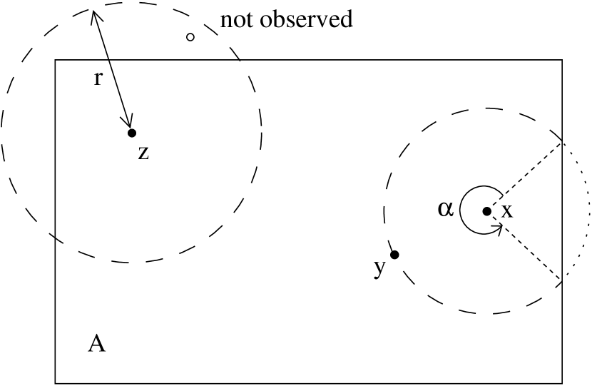
Figure 1: Example of an unobserved point (open dot) within distance $r$ of another point $z$. Also shown is an observed point $y$ within distance $r$ of $x$. This point is given a weight $w(x,|x-y|)$ equal to the reciprocal of the fraction $\alpha/2\pi$ of the circle that is contained within the sample region $A$.

In order to estimate $K(r)$ defined in equation (1), one needs to estimate the average number of neighbors within a distance $r$ of a typical absorber. To understand the problems associated with estimating this quantity, it is helpful to consider the simpler setting of observing a point process in a single contiguous region of space. One possible way to estimate $K(r)$ for a point process observed in a window (or sample region) $A$ with volume $a$ is, for each point in $A$, count how many other points in $A$ are within $r$ of it, sum these counts and then divide by an appropriate quantity that cancels out the effect of the overall intensity of the process. Ripley (1988) calls such an estimator the “naive” estimator. The problem with this estimator is that it tends to underestimate $K(r)$ because for a point within distance $r$ of a boundary of $A$, one may not see all of the points of the process that are within $r$ of it (see Figure 1).

There are a number of methods of correcting for this “edge effect”(Ripley, 1988; Baddeley, 1998; Stein, 1993). In this work, we use the isotropic correction (Ripley, 1988), which is computationally well–suited to the setting of a process observed along lines of sight. To describe this correction, consider the two–dimensional setting pictured in Figure 1. For a point at $x\in A$, if another point $y\in A$ is within distance $r$ of $x$, then instead of giving this event a weight of 1 as in the naive estimator, it is given weight $w(x,|x-y|)$ equal to the reciprocal of the fraction $\alpha/2\pi$ of the circle of radius $|x-y|$ that is contained within $A$ (see Figure 1). As with all of the various edge–correction methods, we then have

$$E\left[\sum_{x\neq y}1\{|x-y|\leq r\}w(x,|x-y|)\right]=\lambda^{2}aK(r)\;,$$ (4)

where $1\{.\}$ is the indicator function, which is unity if the condition in brackets is true and zero otherwise. To estimate $K(r)$, we divide this sum by some estimate of $\lambda^{2}a$. Denoting by $N$ the total number of points observed in $A$, we will use $N(N-1)/a$ as our estimator of $\lambda^{2}a$.

Even recognizing that absorbers have a finite volume, we get to observe absorbers in almost none of the ball of radius $r$ around any absorber, when estimating the three–dimensional $K$ function. Thus, whereas with observations in a single contiguous region, $w(x,|x-y|)$ often equals 1 (i.e., when $x$ is not within $|x-y|$ of the boundary of $A$), for an absorber catalog observed along lines of sight, $w(x,|x-y|)$ will always be much bigger than 1. The exact form of the weight function is given in the Appendix. As one should expect, the weight is inversely proportional to the cross section of the absorbers, or equivalently, to $d^{2}$. Fortunately, our estimator for $\lambda^{2}$ will also be inversely proportional to $d^{2}$, so the factor of $d^{2}$ cancels when estimating $K(r)$.

Quashnock & Stein (1999) used what is known as the rigid–motion estimator to correct for edge effects when estimating the one–dimensional reduced second moment function. To apply the rigid–motion method to an estimate that uses across–line–of–sight information, for every observed distance between pairs of absorbers less than the maximum distance at which we wish to estimate $K$, we would have to apply a three–dimensional rigid motion to the lines of sight, calculate the amount of overlap between the old and new set of lines, and then average this amount over all possible directions. It is not clear how one could do this accurately in practice. Since we have no evidence regarding which estimator is statistically superior in the present setting, we use the computationally much simpler isotropic estimator.

3 Results

We have used equation (A7) and equation (A14) to estimate the reduced second moment measure, $K(r)$, for 276 QSO lines of sight, obtained from the Vanden Berk et al. catalog. A total of 345 C IV absorbers have been selected from this heterogeneous catalog, using selection criteria (Quashnock, Vanden Berk, & York, 1996; Quashnock & Vanden Berk, 1998) designed to obtain as homogeneous a data set as possible. We refer the reader to these papers for a detailed description of the selection criteria.

Figure 2 shows both $\hat{K}_{\parallel}(r)$ (dashed line) and $\hat{K}(r)$ (solid line), divided by their Poisson expectation value, $\text@frac{4}{3}\pi r^{3}$, for the entire C IV absorber catalog. These resultant quantities have expectation value of very nearly unity if there is no clustering of absorbers (see the Appendix). Figure 2 shows that the two estimates agree very well (within their estimated errors, see below) over all distances $r$ from 5 to 300 $h^{-1}$ Mpc, with $\hat{K}_{\parallel}(r)$ just slightly larger than $\hat{K}(r)$ between 30 and 140 $h^{-1}$ Mpc.

Note that, along the same line of sight, the number of absorber pairs separated by very large distances is small, because of the finite comoving length of the lines of sight (the median length is 350 $h^{-1}$ Mpc [Quashnock & Stein 1999]); thus, in Figure 2, for distances $r$ of 170 $h^{-1}$ Mpc and greater, $\hat{K}_{\parallel}(r)$ is noticeably less smooth than $\hat{K}(r)$. Examination of the numbers of absorber pairs along and across lines of sight indicates that it is at such distances that the across line of sight information dominates the total information available. In Table 1, we show the number of absorber pairs in the data set, for pairs along and across lines of sight, as a function of pair separation $r$, in 10 $h^{-1}$ Mpc bins. We also show the cumulative number of pairs for separations $<r$. For pair separations $r>170$ $h^{-1}$ Mpc, there are more additional absorber pairs across different lines of sight than along the same line of sight, whereas for pair separations $r<100$ $h^{-1}$ Mpc, the opposite is true. These two numbers delineate the regimes where, in the Vanden Berk et al. catalog, clustering information arises primarily from pairs across and along lines of sight, respectively. In particular, Table 1 shows that the sample is too sparse to significantly compare clustering along and across lines of sight on scales of less than 100 $h^{-1}$ Mpc.

If the centers of absorbers form a homogeneous Poisson process in three dimensions, i.e., if they are unclustered, then their intersections with the lines of sight form independent one–dimensional Poisson processes, provided their size $d$ is sufficiently small compared to the scales of interest (see Appendix). Thus it is straightforward to simulate the distribution of $\hat{K}_{\parallel}(r)$ and $\hat{K}(r)$ under the assumption that the C IV absorbers are unclustered.

In Figure 3, we show the 95% region of variation about the expectation value of unity of, respectively, $\hat{K}_{\parallel}(r)$ (dashed line) and $\hat{K}(r)$ (solid line), divided by their Poisson expectation value, $\text@frac{4}{3}\pi r^{3}$, for 10,000 simulated data sets of unclustered absorbers with the same arrangement of lines and average number of absorbers as the Vanden Berk et al. catalog. Their averages (dotted lines) are very near the true value of unity, indicating that both estimators are very nearly unbiased in this case. We find that the two estimators have essentially the same region of variation on scales up to $\sim 150$ $h^{-1}$ Mpc; beyond that, the range is smaller for $\hat{K}(r)$, reflecting the additional information contributed by pairs of absorbers across different lines of sight.

To properly interpret the results in Figure 2, one needs some measure of the uncertanties in the estimates. Quashnock & Stein (1999) obtained approximate confidence intervals by bootstrapping, or resampling, lines of sight. Such a procedure makes no use of the relative locations of the lines of sight and is nonsensical when applied to an estimator using across–line–of–sight information. A bootstrapping procedure based on resampling regions of the sky would be more appropriate in the present setting, but the problems of handling edge effects and the uneven spatial distribution of lines of sight complicate matters, so it is unclear how well such a procedure would work.

To provide a rough idea as to the uncertainty of our estimators of $K(r)$, we use a crude but simple approach. We divide the sky into eight regions, each containing nearly the same total length of lines of sight. We then compute the sample standard deviation of the eight estimators of $K(r)$ in the eight regions, assume that the standard deviation $\sigma$ for the estimator based on all of the data will be smaller by a factor of $\sqrt{8}$ and then use the overall estimate plus or minus $2\sigma$ as our confidence interval.

4 Discussion

It is clear that Figure 2 shows strong evidence of clustering on scales up to 100 $h^{-1}$ Mpc ($q_{0}=0.5$), and possibly beyond. In addition, $\hat{K}_{\parallel}(r)$ and $\hat{K}(r)$ essentially agree on the magnitude of the reduced second moment measure up to this distance. This is to be expected, since, as is clear from Table 1, there are very few additional pairs of absorbers coming from different lines of sight on these scales. Thus, the sample is too sparse to significantly compare clustering along and across lines of sight on scales of less than 100 $h^{-1}$ Mpc.

On scales greater than 100 $h^{-1}$ Mpc, however, there are significantly more additional pairs of absorbers from different lines of sight, and it becomes possible to compare their clustering along and across lines of sight. Since $K(r)$ is an integrated measure of clustering on scales from zero to $r$, it is necessary to look at estimates of differential quantities like $K(r_{2})-K(r_{1})$ (with $r_{2}>r_{1}$) in order to examine clustering on scales strictly between $r_{1}$ and $r_{2}$. We have investigated the significance of clustering scales greater than 100 $h^{-1}$ Mpc by examining the quantity

$$\frac{\hat{K}(r_{2})-\hat{K}(r_{1})}{\text@frac{4}{3}\pi(r_{2}^{3}-r_{1}^{3})}-1=\frac{\int_{r_{1}}^{r_{2}}\xi(u)\,u^{2}\,du}{\text@frac{1}{3}(r_{2}^{3}-r_{1}^{3})}\equiv\xi(r_{1},r_{2})\;.$$ (5)

The quantity $\xi(r_{1},r_{2})$ is the estimated average volume–weighted correlation function on scales between $r_{1}$ and $r_{2}$. If the latter two are reasonably close to each other, then $\xi(r_{1},r_{2})$ is an approximate measure of the correlation function $\xi(r)$ on the average scale $r=(r_{1}+r_{2})/2$. Similarly, we define the quantities $\xi_{\parallel}(r_{1},r_{2})$ and $\xi_{\perp}(r_{1},r_{2})$ by replacing $\hat{K}$ in equation (5) above by $\hat{K}_{\parallel}$ and $\hat{K}_{\perp}$, respectively. These two quantities are estimates of the average volume–weighted correlation function that use only along– or cross–line–of–sight information, respectively. We have examined clustering on scales $r$ greater than 100 $h^{-1}$ Mpc by computing $\xi$, $\xi_{\parallel}$, and $\xi_{\perp}$ for a sliding window that is 50 $h^{-1}$ Mpc wide and centered on $r$.

Figure 4 (solid lines) shows all three quantities, $\xi(r-25,r+25)$ (top panel), $\xi_{\perp}(r-25,r+25)$ (middle panel), and $\xi_{\parallel}(r-25,r+25)$ (lower panel), for scales $r$ between 100 $h^{-1}$ Mpc and 300 $h^{-1}$ Mpc. Their approximate 95% regions of variation (again estimated by dividing the QSO sample into eight subsamples corresponding to eight different regions of the sky) are also shown (dashed lines). All three curves are quite similar, showing evidence of clustering on scales $r$ between 100 $h^{-1}$ Mpc and 150 $h^{-1}$ Mpc, and all agree with each other within their approximate confidence regions.

What is particularly striking, however, is that $\xi_{\perp}$ (computed with pairs coming from different lines of sight) essentially agrees within the errors with $\xi_{\parallel}$ (computed with pairs coming from the same line of sight); thus, the additional cross–line–of–sight information strengthens the evidence for clustering on scales from 100 $h^{-1}$ Mpc to 150 $h^{-1}$ Mpc. Although the evidence for clustering across lines of sight is, on its own, only marginally significant, it is consistent with the amplitude and scale of clustering of absorbers along lines of sight; indeed, if anything it hints at being even stronger on these scales.

Such clustering on 100 $h^{-1}$ Mpc to 150 $h^{-1}$ Mpc scales had been hinted at in the one–dimensional work of Quashnock & Stein (1999), and has been confirmed by the three-dimensional analysis here. This argues against claims that all of the apparent line–of–sight clustering on these scales is due to significant contamination along the line of sight by absorbers that are actually physically associated with the QSO (see §1). Figure 4 shows no evidence on clustering on scales between 150 $h^{-1}$ Mpc and 300 $h^{-1}$ Mpc, using any of the three estimators; on scales greater than 150 $h^{-1}$ Mpc, the absorbers appear to be distributed in a manner that is consistent with isotropy. Note that beyond 200 $h^{-1}$ Mpc, $\xi$ has appreciably smaller estimated variability than $\xi_{\parallel}$; this shows how using the full three–dimensional estimator $\hat{K}(r)$ can improve the measurement of clustering on very large scales, even for this modest–sized catalog.

Of course, the lines of sight in the Vanden Berk et al. absorber catalog are rather sparse, and there are still only 345 lines that were analyzed here. The limited size of that catalog, as well as its heterogeneity, precludes a final, strong statement of the statistical significance and amplitude of the clustering on scales between 100 $h^{-1}$ Mpc and 150 $h^{-1}$ Mpc.

As soon as data are available, we will undertake a new effort at analyzing the clustering of heavy–element absorbers in the Sloan Digital Sky Survey (hereafter SDSS), now underway (Margon, 1999). The SDSS QSO Absorption–Line Catalog (hereafter the SDSS Catalog) will include heavy–element absorption–line systems found in the spectra of about 100,000 QSOs, with absorbers ranging in redshift from $z=0.5$ to $z\mathrel{\hbox{\hbox to0.0pt{\hbox{\lower 4.0pt\hbox{$\sim$}}\hss}\hbox{$>$}}}5$. The SDSS Catalog will be of order 300 times larger than the Vanden Berk et al. catalog; furthermore, it will be a homogeneous catalog with fixed selection and detection criteria for the entire sample. Also, the density (number of QSOs per solid angle on the sky) of probing lines of sight will be of order 300 times higher.

Because the SDSS Catalog will have much greater density of lines of sight than the catalog analyzed here, we should expect a much larger fraction of the information about clustering of absorbers from pairs across different lines of sight. Using simulations, we have estimated how much smaller the standard errors of the estimators will be in the 300–times larger SDSS Catalog; in particular, we have investigated how the standard errors will be reduced by using the full three–dimensional estimator and all the cross–line–of–sight information in the 300–times denser SDSS Catalog.

To do this, we have made simulations of randomly placed absorbers and examined how the standard errors of the estimators change if the lines of sight are present at an intensity comparable to that which will be achieved in the SDSS Catalog. We define a region of space similar to that to be probed by the QSO lines of sight of the SDSS Catalog: that section of a cone with half–angle of $45\arcdeg$ and Earth at its tip, which is bounded by comoving distance $2000<r<3300$ $h^{-1}$ Mpc (corresponding to redshift $1.25<z<4$) from Earth. Lines of sight are placed randomly in this region of space, with a uniform distribution of comoving lengths between 250 and 450 $h^{-1}$ Mpc similar to that in the Vanden Berk et al. catalog (Quashnock & Stein, 1999). Mock catalogs were created, with total number, $m$, of lines of sight equal to 100, 1000, 10,000 and 100,000, and absorbers randomly placed on all these lines with the same average number of absorbers per unit comoving length as that observed in the Vanden Berk et al. catalog. The catalogs were generated by simulating a one–dimensional Poisson process on the lines of sight. A set of 10,000 of these unclustered mock catalogs were made for each $m$ except for $m=100{,}000$, for which 100 mock catalogs were made.

The variances of the reduced second moment estimators $\hat{K}_{\parallel}(r)$ and $\hat{K}(r)$ (the average, or expectation value, is, in all cases, very near the true value of $\frac{4}{3}\pi r^{3}$) were computed for each $m$, for $5<r<300$ $h^{-1}$ Mpc. We find, not surprisingly, that the standard error of $\hat{K}_{\parallel}(r)$ decreases with the total number of lines $m$ as $1/\sqrt{m}$; however, this reduction in standard error is constant over $r$. For $\hat{K}(r)$, there is an additional reduction for larger $r$. In Figure 5, we show the ratio of the standard error of $\hat{K}(r)$ for $m=$ 1000 (short-dashed line), 10,000 (long-dashed line), and 100,000 (solid line), to that of $\hat{K}(r)$ for $m=$ 100. As the number of lines of sight increases, there is a continued reduction in the standard error for larger distances, due to the additional and relatively more important number of absorber pairs from across different lines of sight.

This is displayed more dramatically in Figure 6, where we show the relative improvement, or ratio, of the standard errors of $\hat{K}(r)$ to $\hat{K}_{\parallel}(r)$ for $m=$ 100 (dotted line), 1000 (short-dashed line), 10,000 (long-dashed line), and 100,000 (solid line). With 100,000 lines of sight, using $\hat{K}(r)$ instead of $\hat{K}_{\parallel}(r)$ results in an additional factor of 2 to 20 reduction of the standard error on scales of 30 to 200 $h^{-1}$ Mpc, in addition to the factor of $\sqrt{300}$ reduction from the larger sample size, effectively increasing the sample size by an extra factor of 4 to 400 at large distances.

It is the line density (number of lines of sight per solid angle on the sky, or the number of QSOs per square degree) that determines the relative efficiency of $\hat{K}(r)$ to $\hat{K}_{\parallel}(r)$, not the total number of lines $m$. This is also shown in Figure 6, where we show the ratio of the standard errors of $\hat{K}(r)$ to $\hat{K}_{\parallel}(r)$, this time for $m=$ 100 lines of sight, but where the angular density of lines is 10 times (short-dashed and dotted line) and 100 times (long-dashed and dotted line) higher than the initial density; i.e., the solid angle of the conic region described above is 10 and 100 times smaller, respectively. Figure 6 shows that increasing the density of lines by a given factor has the same effect on the relative efficiency of $\hat{K}(r)$ to $\hat{K}_{\parallel}(r)$ as does simply increasing the total number of lines of sight by that same factor. Of course, the overall size of the standard errors is governed by the total number of lines $m$ (see Fig. 5).

These comparisons of the errors in $\hat{K}(r)$ and $\hat{K}_{\parallel}(r)$ are based on unclustered mock catalogs. We are investigating, in ongoing simulations, how different the actual relative improvement might be in a catalog of clustered absorbers such as the SDSS Catalog. Using a simple model of voids and clusters (Loh, 2001) that mimics the correlation structure of the Vanden Berk et al. catalog, we have made 1000 clustered mock catalogs with 100 and 1000 lines of sight. We find, for example, that for $r=$ 300 $h^{-1}$ Mpc, the ratio of the standard errors of $\hat{K}(r)$ to $\hat{K}_{\parallel}(r)$ is 0.629 and 0.230 for unclustered catalogs with 100 and 1000 lines of sight, respectively (see Fig. 6), and 0.669 and 0.270 for clustered catalogs with the same numbers of lines. This indicates that the relative improvement that arises from using cross–line–of–sight pairs in clustered catalogs is still dramatic and is only slightly less so (6% and 17% change in the above two cases) than for unclustered catalogs. Thus, we expect use of the full three–dimensional estimator to substantially increase clustering sensitivity in the SDSS Catalog, with a relative improvement that is only slightly less dramatic than what is shown in Figure 6 (solid line). We hope to present more detailed results elsewhere, with much larger numbers of lines of sight (Loh, 2001).

5 Conclusions

We present two estimators, $\hat{K}_{\parallel}(r)$ and $\hat{K}(r)$, for the three–dimensional reduced second moment for one–dimensional data (absorber redshifts) along QSO lines of sight. The first estimator uses absorber pairs along the same lines of sight, whereas the latter includes data from across different lines of sight. We apply our algorithm to a sample of 345 C IV absorbers with median redshift $\langle z\rangle=2.2$, from the spectra of 276 QSOs, drawn from the catalog of Vanden Berk et al..

We confirm the existence of significant clustering of C IV absorbers on comoving scales up to 100 $h^{-1}$ Mpc ($q_{0}=0.5$), and find that the additional cross–line–of–sight information strengthens the evidence for clustering on scales from 100 $h^{-1}$ Mpc to 150 $h^{-1}$ Mpc. This argues against claims that all the apparent clustering on these scales is due to significant contamination along the line of sight by absorbers that are actually physically associated with the QSO. However, the limited size of that catalog, as well as its heterogeneity, precludes a final, strong statement of the statistical significance and amplitude of the clustering on scales $\mathrel{\hbox{\hbox to0.0pt{\hbox{\lower 4.0pt\hbox{$\sim$}}\hss}\hbox{$>$}}}100$ $h^{-1}$ Mpc. Also, the sample is too sparse to significantly compare clustering along and across lines of sight on scales of less than 100 $h^{-1}$ Mpc. There is no evidence of absorber clustering along or across lines of sight for scales from 150 $h^{-1}$ Mpc to 300 $h^{-1}$ Mpc.

We show that with a 300–times larger catalog, such as that to be compiled by the Sloan Digital Sky Survey (100,000 QSOs), use of the full three–dimensional estimator and cross–line–of–sight information will substantially increase clustering sensitivity. We find that standard errors are reduced by a factor 2 to 20 on scales of 30 to 200 $h^{-1}$ Mpc, in addition to the factor of $\sqrt{300}$ reduction from the larger sample size, effectively increasing the sample size by an extra factor of 4 to 400 at large distances. Thus, use of the full three–dimensional reduced second moment estimator will significantly advance our ability to describe and analyze large–scale clustering of absorbers, and hence visible matter, from the SDSS Catalog.

Appendix A Three–dimensional reduced second moment estimators $\hat{K}_{\parallel}(r)$, $\hat{K}_{\perp}(r)$ and $\hat{K}(r)$

Let $L$ denote the set made up of the $m$ QSO lines of sight, $L_{i}$ the $i$th line, $N$ the total number of absorbers, and $\lambda$ the intensity of the absorber center process, or mean number of absorbers per unit comoving volume. We use $\partial\mathcal{B}_{s}(x,u)$ to represent a shell of inner radius $u$, centered at $x$ and with thickness $s$, $v_{R}(.)$ to indicate measure in $R$ dimensions and $\#\{.\}$ the number of elements in a set. When summing over absorber pairs, we use $\sum^{\parallel}$ to represent a sum over pairs on the same lines of sight only, $\sum^{\perp}$ a sum over pairs across lines of sight only and $\sum$ a sum over all pairs.

We have to give the absorbers some physical size so that there is a non–zero probability of intersection between an absorber and the lines of sight. For simplicity, we assume the absorbers are balls of identical radius $d$. The clustering we seek to measure is the clustering of the point process of the centers of absorbers. Although we do not need to specify $d$, our method requires an approximation that is accurate when $d$ is much smaller than the distances over which we are interested. Define $Q=\pi d^{2}v_{1}(L)$, where $v_{1}(L)$ is the total length of the lines, so $Q$ is effectively the volume of space within which we can observe the center of an absorber.

Throughout we assume that $K(r)$ is continuous in $r$. To estimate $K(r)$, we first estimate $\lambda^{2}QK(r)$ and then divide by an estimate of $\lambda^{2}Q$. Estimating $\lambda^{2}QK(r)$ involves taking each absorber in turn and counting the number of absorbers within a distance $r$. Suppose we have an absorber observed at $x$ on some line of sight. Let another absorber be observed at $y$ on a possibly different line of sight, with $|x-y|\leq r$. Its center must lie within $d$ of $y$. There are generally many other absorbers within $r$ of $x$ that are not observed simply because they lie too far away from the lines of sight. To take into account this edge effect each absorber pair $(x,y)$ is given a weight.

To demonstrate how appropriately chosen weights deal with the problem of edge effects when estimating $\lambda^{2}QK(r)$, we first show that equation (4) of §2.2 holds. Define $1_{(0,r]}(u)=1\{0<u\leq r\}$ and denote the empty set by $\phi$. When observations are in a contiguous window $A$ with volume $a$ and $\partial\mathcal{B}_{0}(x,r)\cap A\neq\phi$ for all $x\in A$,

$$E\left[\sum_{x\neq y}1_{(0,r]}(|x-y|)w(x,|x-y|)\right]$$ (A1)

$$= \lambda^{2}\int_{A}\!\int_{0}^{\infty}\!\int_{\partial\mathcal{B}_{0}(0,1)}1_{(0,r]}(u)1_{A}(x)1_{A}(x+(u,\Omega))w(x,u)u^{2}d\Omega\,dK(u)\,dx$$ (A2)

$$= \lambda^{2}\int_{A}\int_{0}^{\infty}1_{(0,r]}(u)1_{A_{u}}(x)4\pi u^{2}dK(u)\,dx$$ (A3)

$$= \lambda^{2}a\int_{0}^{r}4\pi u^{2}dK(u)$$ (A4)

$$= \lambda^{2}aK(r)$$ (A5)

where in equation (A2), $(u,\Omega)$ are the spherical coordinates of $y-x$. In equation (A3), $A_{u}$ is the set of points in $A$ such that $\partial\mathcal{B}_{0}(x,u)\cap A\neq\phi$, which is simply $A$ when $\partial\mathcal{B}_{0}(x,u)\cap A\neq\phi$ for all $x\in A$.

The step from equation (A3) to (A4) holds only for $u$ less than the circumradius of $A$. Ohser (1983) suggested adding a factor to the estimator so that this step to (A4) is valid at larger distances. This factor is simply the ratio of the volumes of $A$ and $A_{u}$. This extension is not of much practical value when $A$ is a single contiguous region, but it is critical for the line–of–sight catalog, since we would otherwise be restricted to estimating $K$ at distances at most one half the shortest line of sight in the catalog.

Equations (A1)–(A5) demonstrate that estimating $\lambda^{2}aK(r)$ involves taking shells $\partial\mathcal{B}_{du}(x,u)$ with $u<r$ for each point of the process $x\in A$, counting and weighting the number of other points in these shells and integrating over $u$. We now seek to mimic this procedure for absorbers observed along lines of sight. We first consider the simpler case of $\hat{K}_{\parallel}(r)$, in which only pairs of absorbers along the same line of sight are counted. Define $L(x)$ to be the line on which the absorber at $x$ lies. For each pair $(x,y)$ lying on the same line and less than $r$ apart, we set

$$w(x,|x-y|) = 4d^{-2}|x-y|^{2}du/v_{1}(\partial\mathcal{B}_{du}(x,|x-y|)\cap L(x))$$

$$= 4d^{-2}|x-y|^{2}/C_{\parallel}$$

where $C_{\parallel}=C_{\parallel}(x,|x-y|)=\#\{\partial\mathcal{B}_{0}(x,|x-y|)\cap L(x)\}$. In the denominator of equation (A6), $L(x)$ is used and not $L$, since only absorber pairs on the same line of sight are considered. Thus $C_{\parallel}$ takes the value $1$ or $2$. The estimate of $\lambda^{2}QK(r)$ using only absorber pairs on the same line is then

$$\sum\nolimits_{x\neq y}^{\parallel}\frac{1_{(0,r]}(|x-y|)4|x-y|^{2}}{d^{2}C_{\parallel}}\cdot\frac{Q}{\pi d^{2}v_{1}(A^{\parallel}_{|x-y|})}$$

where $A^{\parallel}_{|x-y|}=\cup_{k=1}^{m}\{x\in L_{k}:\partial\mathcal{B}_{0}(x,|x-y|)\cap L_{k}\neq\phi\})$ is the subset of $L$ containing points that are a distance $|x-y|$ from at least one other point on the same line. Ohser’s extension is the factor $\pi d^{2}v_{1}(A^{\parallel}_{|x-y|})/Q$, the proportion of such points in $L$. Taking $N(N-1)/Q$ to be the estimate of $\lambda^{2}Q$, we obtain

$$\hat{K}_{\parallel}(r) = \sum\nolimits_{x\neq y}^{\parallel}\frac{1_{(0,r]}(|x-y|)4|x-y|^{2}}{d^{2}C_{\parallel}}\cdot\frac{Q^{2}}{N(N-1)\pi d^{2}v_{1}(A^{\parallel}_{|x-y|})}$$ (A7)

$$= \sum\nolimits_{x\neq y}^{\parallel}\frac{1_{(0,r]}(|x-y|)4\pi|x-y|^{2}v_{1}(L)^{2}}{C_{\parallel}N(N-1)v_{1}(A^{\parallel}_{|x-y|})}$$

We now show that the estimator of $\lambda^{2}QK(r)$ using pairs along the same line of sight has an unbiasedness property similar to the one found in (A1)–(A5) as $d\to 0$:

$$E\left(\sum\nolimits_{x\neq y}^{\parallel}\frac{1_{(0,r]}(|x-y|)4|x-y|^{2}}{d^{2}C_{\parallel}}\cdot\frac{Q}{\pi d^{2}v_{1}(A^{\parallel}_{|x-y|})}\right)$$ (A8)

$$= \lambda^{2}\int_{{\mathbb{R}}^{3}}\!\int_{0}^{r}\!\int_{\mathcal{B}_{0}(0,1)}\frac{1_{L}(x)1_{L}(x+(u,\Omega))4u^{2}}{d^{2}C_{\parallel}}\cdot\frac{Q}{\pi d^{2}v_{1}(A^{\parallel}_{u})}u^{2}d\Omega\,dK(u)\,dx$$ (A9)

$$= \lambda^{2}Q\int_{{\mathbb{R}}^{3}}\!\int_{0}^{r}\frac{1_{A^{\parallel}_{u}}(x)4u^{2}}{d^{2}C_{\parallel}}\cdot\frac{\pi d^{2}C_{\parallel}+o(d^{2})}{\pi d^{2}v_{1}(A^{\parallel}_{u})}dK(u)dx$$ (A10)

$$= \lambda^{2}Q\int_{0}^{r}\frac{4u^{2}}{d^{2}C_{\parallel}}(\pi d^{2}C_{\parallel}+o(d^{2}))dK(u)$$ (A11)

$$= \lambda^{2}QK(r)+o(d^{2})=\lambda^{2}v_{1}(L)\pi d^{2}K(r)+o(d^{2}).$$ (A12)

Note that when an absorber is observed at $x$ on some line, its center need not be on the line. In fact, this occurs with probability zero. All we can infer is that the center is nearby, at most distance $d$ away. Accordingly, we take $1_{A^{\parallel}_{u}}(x)$ to mean that an absorber center is located so that the center of its interval of intersection with a line of sight is in $A_{u}^{\parallel}$ , and thus the integral over $x$ in (A10) yields $\pi d^{2}v_{1}(A_{u}^{\parallel})$ rather than $v_{1}(A^{\parallel}_{u})$. Since we do not observe exactly where the centers of the absorbers are, all of our estimates of $K(r)$ have some small inherent uncertainty that does not disappear as the size of the observation region increases. Specifically, as the observation region grows, our estimates of $K(r)$ converge to some average of $K(u)$ for $u\in[r-d,r+d]$. This does not pose a problem whenever $r$ is much greater than $d$.

We next derive a similar expression for $\hat{K}_{\perp}(r)$, the estimator for $K(r)$ using only across–line–of–sight information (see §2.2 for a discussion of its validity). For any absorber $x$, we consider absorbers $y$ that lie within a distance $r$ on a different line of sight. Both the assigned weight and Ohser’s extension have to be changed. Define the set $S_{x}=S_{x}(|x-y|)=\partial\mathcal{B}_{0}(x,|x-y|)\cap(L\backslash L(x))$, the set of intersections between $\partial\mathcal{B}_{0}(x,|x-y|)$ and $L\backslash L(x)$. For the absorber pair $(x,y)$, the assigned weight is

$$w(x,|x-y|) = 4d^{-2}|x-y|^{2}du/v_{1}(\partial\mathcal{B}_{du}(x,|x-y|)\cap(L\backslash L(x)))$$

$$= 4d^{-2}|x-y|^{2}/C_{\perp}$$

where $C_{\perp}=C_{\perp}(x,|x-y|)=\sum_{s\in S_{x}}(\cos\theta_{s})^{-1}$ and $\theta_{s}$ is the angle between the line of sight on which $s$ lies and the line joining $s$ and $x$. Figure 7 shows why the factor of $(\cos\theta_{s})^{-1}$ is used. Referring to Figure 7, note that although absorber $y$ is observed on line of sight $k$, the intersection between $\partial\mathcal{B}_{du}(x,u)$ and line of sight $i$ is included in the computation of the weight, since the weight is inversely proportional to the volume of the region in which the appearance of an absorber center would yield an observed location of the absorber in the shell of radius $u$ and thickness $du$ centered at $x$. For an estimator that uses only across–line–of–sight information, the intersection between $\partial\mathcal{B}_{du}(x,u)$ and $L(x)$, the line containing $x$, is not taken into consideration. The estimate of $\lambda^{2}QK(r)$ is

$$\sum\nolimits_{x,y}^{\perp}\frac{1_{(0,r]}(|x-y|)4|x-y|^{2}}{d^{2}C_{\perp}}\cdot\frac{Q}{\pi d^{2}v_{1}(A^{\perp}_{|x-y|})}$$

where $A^{\perp}_{|x-y|}=\cup_{k=1}^{m}\{x\in L_{k}:\partial\mathcal{B}_{0}(x,|x-y|)\cap(L\backslash L_{k})\neq\phi\}$. Ohser’s extension is $\pi d^{2}v_{1}(A^{\perp}_{|x-y|})/Q$ and is the proportion of points in $L$ that are a distance $|x-y|$ from at least one other point on another line. This yields as an estimate of $K(r)$,

$$\hat{K}_{\perp}(r)=\sum\nolimits_{x,y}^{\perp}\frac{1_{(0,r]}(|x-y|)4\pi|x-y|^{2}v_{1}(L)^{2}}{C_{\perp}N(N-1)v_{1}(A^{\perp}_{|x-y|})}$$ (A13)

With appropriate changes, i.e. $C_{\parallel}$ and $A^{\parallel}_{u}$ replaced by $C_{\perp}$ and $A^{\perp}_{u}$, steps (A8)–(A12) hold for $\hat{K}_{\perp}(r)-\hat{K}_{\perp}(r_{0})$, where $r_{0}$ is the shortest distance between different lines of sight in the catalog.

The estimate of $K(r)$ which uses all absorber pairs is now not difficult to obtain. This estimate is not simply a sum of $\hat{K}_{\parallel}(r)$ and $\hat{K}_{\perp}(r)$. It is true that it involves a sum of all absorber pairs, both along and across lines of sight. However, in each term of the sum, the expression for Ohser’s extension and the assigned weight are different. For absorber pair $(x,y)$, the probed volume that contributes to the weight is now a sum of that probed by $L(x)$ and $L\backslash L(x)$: $w(x,|x-y|)=4d^{-2}|x-y|^{2}/(C_{\parallel}+C_{\perp})$. The set of points with at least one other point $|x-y|$ away is now a union of the two sets $A^{\parallel}_{|x-y|}$ and $A^{\perp}_{|x-y|}$, which is $A_{|x-y|}$. With these adjustments, we have

$$\hat{K}(r)=\sum\nolimits_{x\neq y}\frac{1_{(0,r]}(|x-y|)4\pi|x-y|^{2}v_{1}(L)^{2}}{(C_{\parallel}+C_{\perp})N(N-1)v_{1}(A^{\parallel}_{|x-y|}\cup A^{\perp}_{|x-y|})}.$$ (A14)

Even when using $\hat{K}(r)$, the fraction of volume of $\partial\mathcal{B}_{du}(x,u)$ probed by the absorber catalog is very small and thus the weights are always much larger than $1$. Nevertheless, even in the moderate size catalog used here, there is sufficient information to enable us to obtain useful estimates of the three-dimensional reduced second moment measure at large distances.

Figure 2: Estimates of the reduced second moment measure, $\hat{K}_{\parallel}(r)$ (dashed line) and $\hat{K}(r)$ (solid line), divided by their Poisson expectation $\text@frac{4}{3}\pi r^{3}$, together with the latter’s approximate 95% confidence region (dotted line; see text), for the 276 QSO lines of sight, containing a total of 345 C IV absorbers obtained from the Vanden Berk et al. catalog.

Figure 3: The 95% regions of variation of $\hat{K}_{\parallel}(r)$ (dashed line) and $\hat{K}(r)$ (solid line), divided by their Poisson expectation value, $\text@frac{4}{3}\pi r^{3}$, for 10,000 simulated data sets of unclustered absorbers with the same total number of lines and average number of absorbers as the Vanden Berk et al. catalog. The averages for both estimators (dotted lines) are very near their expectation value of unity.

Figure 4: Average volume–weighted correlation functions (solid lines) $\xi(r-25,r+25)$ (top panel), $\xi_{\perp}(r-25,r+25)$ (middle panel), and $\xi_{\parallel}(r-25,r+25)$ (bottom panel), for $100<r<300$ $h^{-1}$ Mpc, for the 276 QSO lines of sight and 345 C IV absorbers of the Vanden Berk et al. catalog. Their approximate 95% regions of variation are also shown (dashed lines; see text).

Figure 5: Ratio of the standard errors of $\hat{K}(r)$ for $m=$ 1000 (short-dashed line), 10,000 (long-dashed line), and 100,000 (solid line), to that of $\hat{K}(r)$ for $m=$ 100, for mock unclustered catalogs. Note the continued reduction in the standard error on larger scales.

Figure 6: Ratio of the standard errors of $\hat{K}(r)$ to $\hat{K}_{\parallel}(r)$ for $m=$ 100 (dotted line), 1000 (short-dashed line), 10,000 (long-dashed line), and 100,000 (solid line), with mock unclustered catalogs. Also shown is the same ratio, for $m=$ 100 lines of sight, but where the angular density of lines is 10 times higher (short-dashed and dotted line) and 100 times higher (long-dashed and dotted line).

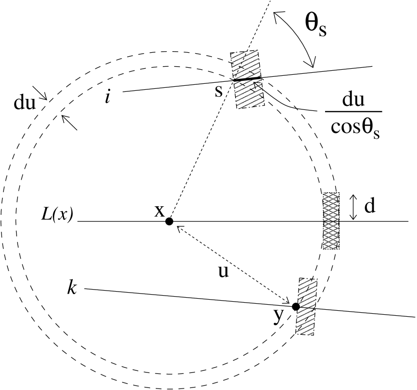
Figure 7: Schematic showing how to obtain the weights for $\hat{K}_{\perp}(r)$ and $\hat{K}(r)$ in a two–dimensional setting. Absorbers are observed at $x$ and $y$, and are separated by distance $u=|x-y|\leq r$; $d$ is the assumed radius of all absorbers. For $\hat{K}_{\perp}(r)$, the weight $w(x,y)$ is inversely proportional to the sum of the volumes of the two singly hatched regions. Note that the thickness of the shaded region through line of sight $i$ is $dr/\cos\theta_{s}$. For $\hat{K}(r)$, the weight $w(x,y)$ is inversely proportional to the sum of the volumes of the three hatched regions.

Table 1: Number of absorber pairs as a function of pair separation $r$

	Number in bin			Cumulative Number
$r$ ($h^{-1}$ Mpc)	along lines	across lines		along lines	across lines
10	63	0		63	0
20	21	8		84	8
30	26	5		110	13
40	30	3		140	16
50	22	5		162	21
60	31	3		193	24
70	17	5		210	29
80	17	7		227	36
90	11	3		238	39
100	15	6		253	45
110	9	16		262	61
120	16	9		278	70
130	12	10		290	80
140	14	8		304	88
150	13	9		317	97
160	6	7		323	104
170	18	11		341	115
180	2	15		343	130
190	10	9		353	139
200	6	13		359	152
210	2	16		361	168
220	3	19		364	187
230	4	15		368	202
240	8	9		376	211
250	2	10		378	221
260	5	9		383	230
270	1	12		384	242
280	5	17		389	259
290	4	18		393	277
300	1	16		394	293

References

- Baddeley (1998) Baddeley, A. 1998, in Stochastic Geometry: Likelihood and Computation, eds. O. E. Barndorff-Nielsen, W. S. Kendall, & M. N. M. van Lieshout (London: Chapman and Hall), ch. 2
- Churchill, Steidel, & Vogt (1996) Churchill, C. W., Steidel, C. C., & Vogt, S. S. 1996, ApJ, 471, 164
- Cristiani et al. (1997) Cristiani, S., D’Odorico, S., D’Odorico, V., Fontana, A., Giallongo, E., & Savaglio, S. 1997, MNRAS, 285, 209
- Crotts, Burles, & Tytler (1997) Crotts, A. P. S., Burles, S., & Tytler, D. 1997, ApJ, 489, L7
- D’Odorico et al. (1998) D’Odorico, V., Cristiani, S., D’Odorico, S., Fontana, A., Giallongo, E., & Shaver, P. 1998, A&A, 339, 678
- Loh (2001) Loh, J. M. 2001, Ph.D. thesis (University of Chicago)
- Margon (1999) Margon, B. 1999, Phil. Trans. R. Soc. Lond., A 357, 93
- Martínez et al. (1998) Martínez, V. J., Pons-Bordería, M.-J., Moyeed, R. A., & Graham, M. J. 1998, MNRAS, 298, 1212
- Ohser (1983) Ohser, J. 1983, Math. Oper. Statist. ser Statist. 14, 63
- Peebles (1980) Peebles, P. J. E. 1980, The Large–Scale Structure of the Universe (Princeton: Princeton Univ. Press)
- Peebles (1993) Peebles, P. J. E. 1993, Principles of Physical Cosmology (Princeton: Princeton Univ. Press)
- Quashnock, Vanden Berk, & York (1996) Quashnock, J. M., Vanden Berk, D. E., & York, D. G. 1996, ApJ, 472, L69
- Quashnock & Vanden Berk (1998) Quashnock, J. M., & Vanden Berk, D. E. 1998, ApJ, 500, 28
- Quashnock & Stein (1999) Quashnock, J. M., & Stein, M. L. 1999, ApJ, 515, 506
- Richards et al. (1999) Richards, G. T., York, D. G., Yanny, B., Kollgaard, R. I., Laurent-Muehleisen, S. A., & Vanden Berk, D. E. 1999, ApJ, 513, 576
- Ripley (1988) Ripley, B. D. 1988, Statistical Inference for Spatial Processes (Cambridge: Cambridge Univ. Press)
- Stein (1993) Stein, M. L. 1993, Biometrika, 80, 443
- Stein, Quashnock, & Loh (2000) Stein, M. L., Quashnock, J. M., & Loh, J. M. 2000, Ann. Stat. (in press) (physics/0006047)
- Vanden Berk et al. (1996) Vanden Berk, D. E., Quashnock, J. M., York, D. G., & Yanny, B. 1996, ApJ, 469, 78
- York et al. (1991) York, D. G., Yanny, B., Crotts, A., Carilli, C., Garrison, E., & Matheson, L. 1991, MNRAS, 250, 24