The Quintessential CMB, Past & Future

Abstract

The past, present and future of cosmic microwave background (CMB) anisotropy research is discussed, with emphasis on the Boomerang and Maxima balloon experiments. These data are combined with large scale structure (LSS) information derived from local cluster abundances and galaxy clustering and high redshift supernova (SN1) observations to explore the inflation-based cosmic structure formation paradigm. Here we primarily focus on a simplified inflation parameter set, $\{\omega_{b},\omega_{cdm},\Omega_{tot},\Omega_{Q},w_{Q},n_{s},\tau_{C},\sigma_{8}\}$. After marginalizing over the other cosmic and experimental variables, we find the current CMB+LSS+SN1 data gives $\Omega_{tot}=1.04\pm 0.05$, consistent with (non-baroque) inflation theory. Restricting to $\Omega_{tot}=1$, we find a nearly scale invariant spectrum, $n_{s}=1.03\pm 0.07$. The CDM density, $\omega_{cdm}=0.17\pm 0.02$, is in the expected range, but the baryon density, $\omega_{b}\equiv\Omega_{b}{\rm h}^{2}=0.030\pm 0.004$, is slightly larger than the current $0.019\pm 0.002$ Big Bang Nucleosynthesis estimate. Substantial dark (unclustered) energy is inferred, $\Omega_{Q}\approx 0.68\pm 0.05$, and CMB+LSS $\Omega_{Q}$ values are compatible with the independent SN1 estimates. The dark energy equation of state, parameterized by a quintessence-field pressure-to-density ratio $w_{Q}$, is not well determined by CMB+LSS ($w_{Q}<-0.3$ at 95% CL), but when combined with SN1 the resulting $w_{Q}<-0.7$ limit is quite consistent with the $w_{Q}$=$-1$ cosmological constant case. Though forecasts of statistical errors on parameters for current and future experiments are rosy, rooting out systematic errors will define the true progress.

CMB Analysis: Past, Present and Future

The CMB is a nearly perfect blackbody of $2.725\pm 0.002\,K$ matherTcmb , with a $3.372\pm 0.007\,mK$ dipole associated with the 300 ${\rm~{}km~{}s^{-1}}$ flow of the earth in the CMB, and a rich pattern of higher multipole anisotropies at tens of $\mu$K arising from fluctuations at photon decoupling and later. Spectral distortions from the blackbody associated with starbursting galaxies detected in the COBE FIRAS and DIRBE data are due to stellar and accretion disk radiation being downshifted into the infrared by dust then redshifted into the submillimetre; they have energy about twice all that in optical light, about a tenth of a percent of that in the CMB. The spectrally well-defined Sunyaev-Zeldovich (SZ) distortion associated with Compton-upscattering of CMB photons from hot gas has not been observed with FIRAS, but only at high resolution along lines-of-sight through dozens of clusters — with very high signal-to-noise though. The FIRAS 95% CL upper limit of $6.0\times 10^{-5}$ of the energy in the CMB is compatible with the $\mathrel{\hbox to0.0pt{\lower 3.0pt\hbox{$\mathchar 536\relax$}\hss}\raise 2.0pt\hbox{$\mathchar 316\relax$}}10^{-5}$ expected from clusters, groups and filaments in structure formation models, and places strong constraints on the allowed amount of earlier energy injection, e.g., ruling out mostly hydrodynamic models of LSS.

Upper Limit Experiments from the 70s & 80s: The story of the experimental quest for anisotropies is a heroic one. The original 1965 Penzias and Wilson discovery paper quoted angular anisotropies below $10\%$, but by the late sixties $10^{-3}$ limits were reached, by Partridge and Wilkinson and by Conklin and Bracewell. As calculations of baryon-dominated adiabatic and isocurvature models improved in the 70s and early 80s, the theoretical expectation was that the experimentalists just had to get to $10^{-4}$, as they did, e.g., Boynton and Partridge in 73. The only signal found was the dipole, hinted at by Conklin and Bracewell in 73, but found definitively in Berkeley and Princeton balloon experiments in the late 70s, along with upper limits on the quadrupole. Throughout the 1980s, the upper limits kept coming down, punctuated by a few experiments widely used by theorists to constrain models: the small angle 84 Uson and Wilkinson and 87 OVRO limits, the large angle 81 Melchiorri limit, early (87) limits from the large angle Tenerife experiment, the small angle RATAN-600 limits, the $7^{\circ}$-beam Relict-1 satellite limit of 87, and Lubin and Meinhold’s 89 half-degree South Pole limit, marking a first assault on the peak.

These upper limit experiments were highly useful, in particular to rule out adiabatic baryon-dominated models. In the early 80s, dark matter dominated universes lowered theoretical predictions by about an order of magnitude. In the 84 to mid-90s period, many groups developed codes to solve the perturbed Boltzmann–Einstein equations when dark matter was present. Armed with these pre-COBE computations, plus the LSS information of the time, a number of very interesting models fell victim to the data: scale invariant isocurvature cold dark matter models in 86, large regions of parameter space for isocurvature baryon models in 87, inflation models with radically broken scale invariance leading to enhanced power on large scales in 87-89, CDM models with a decaying ($\sim{\rm keV}$) neutrino if its lifetime was too long ($\mathrel{\hbox to0.0pt{\lower 3.0pt\hbox{$\mathchar 536\relax$}\hss}\raise 2.0pt\hbox{$\mathchar 318\relax$}}10{\rm yr}$) in 87 and 91. Also in this period there were some limited constraints on ”standard” CDM models, restricting $\Omega_{tot}$, $\Omega_{B}$, and the amplitude parameter $\sigma_{8}$. ($\sigma_{8}^{2}$ is a bandpower for density fluctuations on a scale associated with rare clusters of galaxies, $8{\,{\rm h}^{-1}~{}\rm Mpc}$, where ${\rm h}=H_{0}/(100{\rm~{}km~{}s^{-1}}{\rm~{}Mpc}^{-1})$.)

Post-DMR Experiments: The now familiar motley pattern of anisotropies associated with $2\mathrel{\hbox to0.0pt{\lower 3.0pt\hbox{$-$}\hss}\raise 2.0pt\hbox{$\mathchar 316\relax$}}\ell\mathrel{\hbox to0.0pt{\lower 3.0pt\hbox{$\mathchar 536\relax$}\hss}\raise 2.0pt\hbox{$\mathchar 316\relax$}}20$ multipoles at the $30\mu K$ level revealed by COBE at $7^{\circ}$ resolution was shortly followed by detections, and a few upper limits (UL), at higher $\ell$ in 19 other ground-based (gb) or balloon-borne (bb) experiments — most with many fewer resolution elements than the 600 or so for COBE. Some predated in design and even data delivery the 1992 COBE announcement. Proceeding from the period we began analyzing them, we have the intermediate angle SP91 (gb), the large angle FIRS (bb), both with strong hints of detection before COBE, then, post-COBE, more Tenerife (gb), MAX (bb), MSAM (bb), white-dish (gb, UL), argo (bb), SP94 (gb), SK93-95 (gb), Python (gb), BAM (bb), CAT (gb), OVRO-22 (gb), SuZIE (gb, UL), QMAP (bb), VIPER (gb) and Python V (gb). A list valid to April 1999 with associated bandpowers is given in bjk9800 , and are referred here as 4.99 data. They showed evidence for a first peak bjk9800 , although it was not well localized. Within limited parameter sets, good constraints on $n_{s}$, some on $\Omega_{tot}$ and $\Omega_{\Lambda}$ could be given, when LSS was added.

The Present, TOCO, BOOMERANG & MAXIMA: The picture dramatically improved this year, as results were announced first in summer 99 from the ground-based TOCO experiment in Chile toco98 , then in November 99 from the North American balloon test flight of Boomerang mauskopf99 . These two additions improved peak localization and gave evidence for $\Omega_{tot}\sim 1$. Then in April 2000 results from the first CMB long duration balloon (LDB) flight, Boomerang debernardis00 , were announced, followed in May 2000 by results from the night flight of Maxima MAXIMA1 . Boomerang’s best resolution was $10^{\prime}$, about 40 times better than that of COBE, with tens of thousands of resolution elements. Maxima had a similar resolution but covered an order of magnitude less sky.

Boomerang carried a 1.2m telescope with 16 bolometers cooled to 300 mK in the focal plane aloft from McMurdo Bay in Antarctica in late December 1998, circled the Pole for 10.6 days and landed just 50 km from the launch site, only slightly damaged. In debernardis00 , maps at 90, 150 and 220 GHz showed the same spatial features and the intensities were shown to fall precisely on the CMB blackbody curve. The fourth frequency channel at 400 GHz is dust-dominated. Fig. 1 shows the 150 GHz map derived using only one of the 16 bolometers. Although Boomerang altogether probed 1800 square degrees, only the region in the rectangle covering 440 square degrees was used in the analysis described in lange00 ; jaffe00 and this paper. Fig. 1 also shows the 124 square degree region of the sky (in the Northern Hemisphere) that Maxima-1 probed. Though Maxima was not an LDB, it did so well because its bolometers were cooled even more than Boomerang’s, to 100 mK, leading to higher sensitivity per unit observing time, it had a star camera so the pointing was well determined, and, further, all frequency channels were used in creating its map.

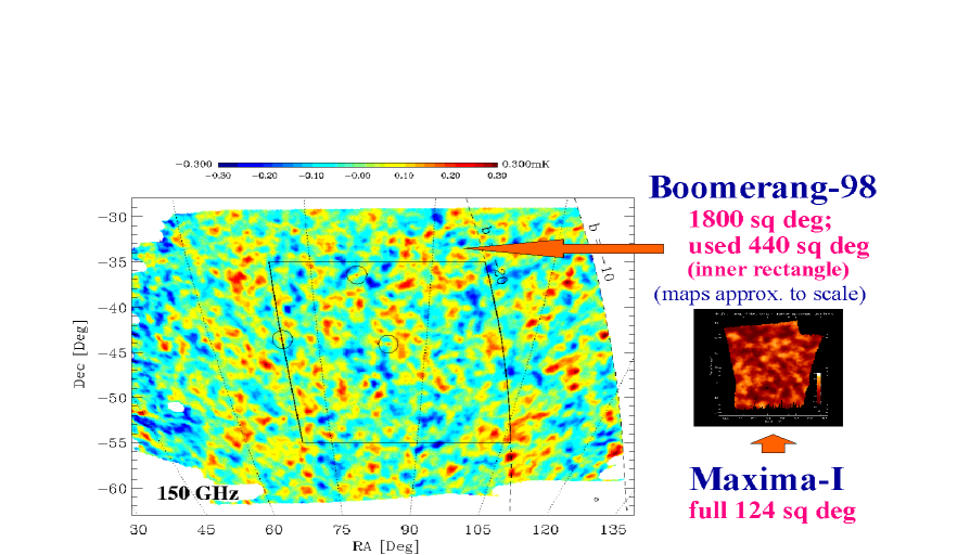
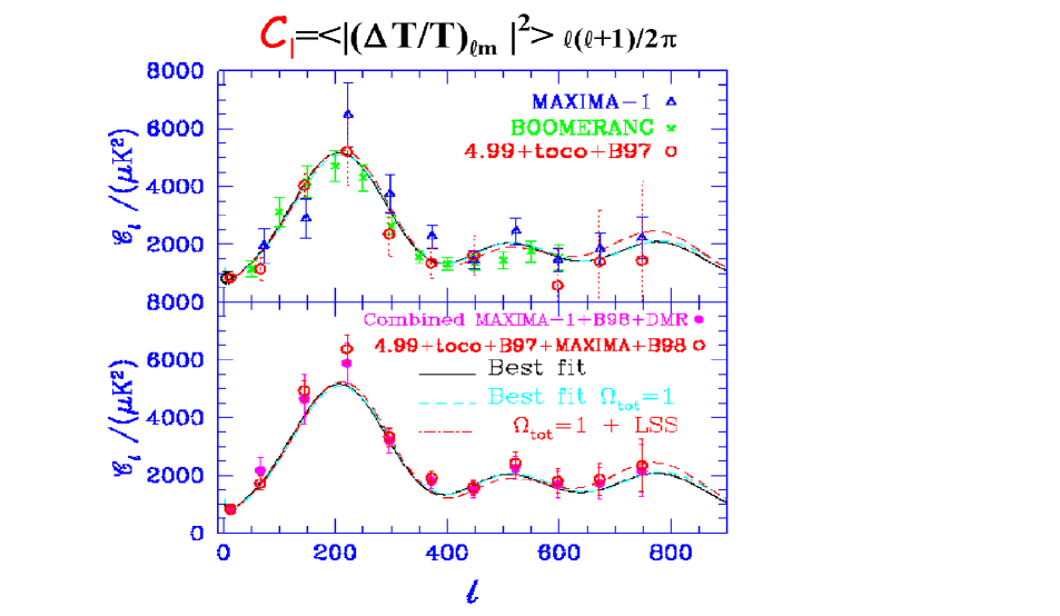
Figure 1: The Boomerang 150A GHz bolometer map (one out of 16) is shown in the top figure. Of the entire 1800 square degrees covered, only the interior 440 sq. degs. (within the central rectangle) were used in our analysis, i.e., in all less than 5% of the data. The 124 square degree Maxima-I map, drawn to scale, is also shown. In the lower figure, the ${\cal C}_{\ell}$ (defined in terms of CMB temperature anisotropy multipoles, $(\Delta T/T)_{\ell m}$, as indicated) grouped in bandpowers for prior-CMB experiments, including TOCO and the North American Boomerang test flight, (squares) are contrasted with the Boomerang-LDB (crosses) and Maxima-I (triangles) results in the upper panel. The lower panel shows the optimally-combined power spectra of Boomerang+Maxima+prior-CMB (circles) and contrasts it with that for Boomerang+Maxima+DMR (squares), showing that including the prior experiments does not make a large difference to the results. Best-fit models for arbitrary $\Omega_{tot}$ and for $\Omega_{tot}$=1 are shown in both panels.

Primary CMB Processes and Soundwave Maps at Decoupling: Both Boomerang and Maxima were designed to measure the primary anisotropies of the CMB, those which can be calculated using linear perturbation theory. What we see in Fig. 1 are, basically, two images of soundwave patterns that existed about 300,000 years after the Big Bang, when the photons were freed from the plasma. The visually evident structure on degree scales is even more apparent in the power spectra of the Fourier transform of the maps, which show a dominant (first acoustic) peak, a less prominent (or non-existent) second one, and the possible hint of a third one from Maxima. Fig. 1 also shows that the quite heterogeneous 4.99+TOCO+Boomerang-NA mix of CMB data is very consistent with what Boomerang-LDB and Maxima show.

The images are actually a projected mixture of dominant and subdominant physical processes through the photon decoupling ”surface”, a fuzzy wall at redshift $z_{r}\sim 1100$, when the Universe passed from optically thick to thin to Thomson scattering over a comoving distance $\sim 10{\,{\rm h}^{-1}~{}\rm Mpc}$. Prior to this, acoustic wave patterns in the tightly-coupled photon-baryon fluid on scales below the comoving ”sound crossing distance” at decoupling, $\mathrel{\hbox to0.0pt{\lower 3.0pt\hbox{$\mathchar 536\relax$}\hss}\raise 2.0pt\hbox{$\mathchar 316\relax$}}100{\,{\rm h}^{-1}~{}\rm Mpc}$ (i.e., $\mathrel{\hbox to0.0pt{\lower 3.0pt\hbox{$\mathchar 536\relax$}\hss}\raise 2.0pt\hbox{$\mathchar 316\relax$}}100{\rm~{}kpc}$ physical), were viscously damped, strongly so on scales below the $\sim 10{\,{\rm h}^{-1}~{}\rm Mpc}$ thickness over which decoupling occurred. After, photons freely-streamed along geodesics to us, mapping (through the angular diameter distance relation) the post-decoupling spatial structures in the temperature to the angular patterns we observe now as the primary CMB anisotropies. The maps are images projected through the fuzzy decoupling surface of the acoustic waves (photon bunching), the electron flow (Doppler effect) and the gravitational potential peaks and troughs (”naive” Sachs-Wolfe effect) back then. Free-streaming along our (linearly perturbed) past light cone leaves the pattern largely unaffected, except that temporal evolution in the gravitational potential wells as the photons propagate through them leaves a further $\Delta T$ imprint, called the integrated Sachs-Wolfe effect. Intense theoretical work over three decades has put accurate calculations of this linear cosmological radiative transfer on a firm footing, and there is a speedy, publicly available and widely used code for evaluation of anisotropies in a variety of cosmological scenarios, “CMBfast” cmbfast , including the latest hydrogen/helium recombination evaluations, and with extensions to more cosmological models added by a variety of researchers.

Of course there are a number of nonlinear effects that are also present in the maps. These secondary anisotropies include weak-lensing by intervening mass, Thompson-scattering by the nonlinear flowing gas once it became ”reionized” at $z\sim 20$, the thermal and kinematic SZ effects, and the red-shifted emission from dusty galaxies. They all leave non-Gaussian imprints on the CMB sky.

The Future, beyond 2000: We are only at the beginning of the high precision CMB era. HEMT-based interferometers are already in place taking data: the VSA (Very Small Array) in Tenerife, the CBI (Cosmic Background Imager) in Chile, DASI (Degree Angular Scale Interferometer) at the South Pole, where the bolometer-based single dish ACBAR experiment will operate this year. Other LDBs will be flying within the next few years: Arkeops, Tophat, Beast/Boost; and in 2001, Boomerang will fly again, this time concentrating on polarization. As well, MAXIMA will fly as the polarization-targeting MAXIPOL. In April 2001, NASA will launch the all-sky HEMT-based MAP satellite, with $12^{\prime}$ resolution. Further downstream, in 2007, ESA will launch the bolometer+HEMT-based Planck satellite, with $5^{\prime}$ resolution.

Secondary anisotropies are also being targeted with new instruments. SZ anisotropies have been probed by single dishes, the OVRO and BIMA mm arrays, and the Ryle interferometer. A number of planned HEMT-based interferometers being built are more ambitious: AMI (Britain), the JCA (Chicago), AMIBA (Taiwan), MINT (Princeton). As well other kinds of bolometer-based experiments will be used to probe the SZ effect, including the CSO (Caltech submm observatory) with BOLOCAM on Mauna Kea, ACBAR at the South Pole, the LMT (large mm telescope) in Mexico, and the LDB BLAST. Anisotropies from dust emission from high redshift galaxies are being targeted by the JCMT with the SCUBA bolometer array, the OVRO mm interferometer, the CSO, the SMA (submm array) on Mauna Kea, the LMT, the ambitious US/ESO ALMA mm array in Chile, the LDB BLAST, and ESA’s FIRST satellite. About $50\%$ of the submm background has so far been identified with sources that SCUBA has found.

The CMB Analysis Pipeline: Analyzing Boomerang and other experiments involves a pipeline that takes (1) the timestream in each of the bolometer channels coming from the balloon plus information on where it is pointing and turns it into (2) spatial maps for each frequency characterized by average temperature fluctuation values in each pixel (Fig. 1) and a pixel-pixel correlation matrix characterizing the noise, from which various statistical quantities are derived, in particular (3) the temperature power spectrum as a function of multipole (Fig. 1), grouped into bands, and two band-band error matrices which together determine the full likelihood distribution of the bandpowers bjk9800 . Fundamental to the first step is the extraction of the sky signal from the noise, using the only information we have, the pointing matrix mapping a bit in time onto a pixel position on the sky.

There is generally another step in between (2) and (3), namely separating the multifrequency spatial maps into the physical components on the sky: the primary CMB, the thermal and kinematic Sunyaev-Zeldovich effects, the dust, synchrotron and bremsstrahlung Galactic signals, the extragalactic radio and submillimetre sources. The strong agreement among the Boomerang maps indicates that to first order we can ignore this step, but it has to be taken into account as the precision increases. The Fig. 1 map is consistent with a Gaussian distribution, thus fully characterized by just the power spectrum. Higher order (concentration) statistics (3,4-point functions, etc.) tell us of non-Gaussian aspects, necessarily expected from the Galactic foreground and extragalactic source signals, but possible even in the early Universe fluctuations. For example, though non-Gaussianity occurs only in the more baroque inflation models of quantum noise, it is a necessary outcome of defect-driven models of structure formation. (Peaks compatible with Fig. 1 do not appear in non-baroque defect models, which now appear unlikely.) Though great strides have been made in the analysis of Boomerang and Maxima, there is intense needed effort worldwide now to develop new fast algorithms to deal with the looming megapixel datasets of LDBs and the satellites bcjk99szapudi00 .

Cosmic Parameter Estimation

Parameters of Structure Formation: For this paper, we adopt a restricted set of 8 cosmological parameters, augmenting the basic 7 used in lange00 ; jaffe00 , $\{\Omega_{\Lambda},\Omega_{k},\omega_{b},\omega_{cdm},n_{s},\tau_{C},\sigma_{8}\}$, by one. The vacuum or dark energy encoded in the cosmological constant $\Omega_{\Lambda}$ is reinterpreted as $\Omega_{Q}$, the energy in a scalar field $Q$ which dominates at late times, which, unlike $\Lambda$, could have complex dynamics associated with it. $Q$ is now often termed a quintessence field - see http://feynman.princeton.edu/ steinh/ ”Quintessence? - an overview” for a pedagogical introduction. One popular phenomenology is to add one more parameter, $w_{Q}=p_{Q}/\rho_{Q}$, where $p_{Q}$ and $\rho_{Q}$ are the pressure and density of the $Q$-field, related to its kinetic and potential energy by $\rho_{Q}=\dot{Q}^{2}/2+(\nabla Q)^{2}/2+V(Q)$, $p_{Q}=\dot{Q}^{2}/2-(\nabla Q)^{2}/6-V(Q)$. Thus $w_{Q}=-1$ for the cosmological constant. Spatial fluctuations of $Q$ are expected to leave a direct imprint on the CMB for small $\ell$, typically smaller than Boomerang or Maxima are sensitive to. We ignore this complication here. As well, as long as $w_{Q}$ is not exactly $-1$, it will vary with time, but the data will have to improve for there to be sensitivity to this, and for now we can just interpret $w_{Q}$ as an appropriate time-average of the equation of state. The curvature energy $\Omega_{k}\equiv 1-\Omega_{tot}$ also can dominate at late times, as well as affecting the geometry.

We use only 2 parameters to characterize the early universe primordial power spectrum of gravitational potential fluctuations $\Phi$, one giving the overall power spectrum amplitude ${\cal P}_{\Phi}(k_{n})$, and one defining the shape, a spectral tilt $n_{s}(k_{n})\equiv 1+d\ln{\cal P}_{\Phi}/d\ln k$, at some (comoving) normalization wavenumber $k_{n}$. We really need another 2, ${\cal P}_{GW}(k_{n})$ and $n_{t}(k_{n})$, associated with the gravitational wave component. In inflation, the amplitude ratio is related to $n_{t}$ to lowest order, with ${\cal O}(n_{s}-n_{t})$ corrections at higher order, e.g., bh95 . There are also useful limiting cases for the $n_{s}-n_{t}$ relation. However, as one allows the baroqueness of the inflation models to increase, one can entertain essentially any power spectrum (fully $k$-dependent $n_{s}(k)$ and $n_{t}(k)$) if one is artful enough in designing inflaton potential surfaces. As well, one can have more types of modes present, e.g., scalar isocurvature modes (${\cal P}_{is}(k_{n}),n_{is}(k)$) in addition to, or in place of, the scalar curvature modes (${\cal P}_{\Phi}(k_{n}),n_{s}(k)$). However, our philosophy is consider minimal models first, then see how progressive relaxation of the constraints on the inflation models, at the expense of increasing baroqueness, causes the parameter errors to open up. For example, with COBE-DMR and Boomerang, we can probe the GW contribution, but the data are not powerful enough to determine much. Planck can in principle probe the gravity wave contribution reasonably well.

We use another 2 parameters to characterize the transport of the radiation through the era of photon decoupling, which is sensitive to the physical density of the various species of particles present then, $\omega_{j}\equiv\Omega_{j}{\rm h}^{2}$. We really need 4: $\omega_{b}$ for the baryons, $\omega_{cdm}$ for the cold dark matter, $\omega_{hdm}$ for the hot dark matter (massive but light neutrinos), and $\omega_{er}$ for the relativistic particles present at that time (photons, very light neutrinos, and possibly weakly interacting products of late time particle decays). For simplicity, though, we restrict ourselves to the conventional 3 species of relativistic neutrinos plus photons, with $\omega_{er}$ therefore fixed by the CMB temperature and the relationship between the neutrino and photon temperatures determined by the extra photon entropy accompanying $e^{+}e^{-}$ annihilation. Of particular importance for the pattern of the radiation is the (comoving) distance sound can have influenced by recombination (at redshift $z_{r}=a_{r}^{-1}-1$), $r_{s}=6000/\sqrt{3}{\rm~{}Mpc}\int_{0}^{\sqrt{a_{r}}}(\omega_{m}+\omega_{er}a^{-1})^{-1/2}(1+\omega_{b}a/(4\omega_{\gamma}/3))^{-1/2}\ d\sqrt{a}$, where $\omega_{\gamma}=2.46\times 10^{-5}$ is the photon density, $\omega_{er}=1.68\omega_{\gamma}$ for 3 species of massless neutrinos and $\omega_{m}\equiv\omega_{hdm}+\omega_{cdm}+\omega_{b}$.

The angular diameter distance relation, ${\cal R}=\{d_{k}{\rm sinh}(\chi_{r}/d_{k}),\chi_{r},d_{k}{\rm sin}(\chi_{r}/d_{k})\}$, where $\chi_{r}=6000{\rm~{}Mpc}\int_{\sqrt{a_{r}}}^{1}(\omega_{m}+\omega_{Q}a^{-6w_{Q}}+\omega_{k}a)^{-1/2}\ d\sqrt{a}$ is the comoving distance to recombination, $d_{k}=3000|\omega_{k}|^{-1/2}{\rm~{}Mpc}$ is the curvature scale and the 3 cases are for negative, zero and positive mean curvature, adds dependence upon $\omega_{k}$, $\omega_{Q}$ and $w_{Q}$ as well as on $\omega_{m}$. The location of the first acoustic peak $L_{Pk}$ is proportional to the ratio of ${\cal R}$ to $r_{s}$, hence depends upon $\omega_{b}$ through the sound speed as well. Thus $L_{Pk}$ defines a functional relationship among these parameters, a degeneracy degeneracies that would be exact except for the integrated Sachs-Wolfe effect, associated with the change of $\Phi$ with time if $\Omega_{Q}$ or $\Omega_{k}$ is nonzero. (If $\dot{\Phi}$ vanishes, the energy of photons coming into potential wells is the same as that coming out, and there is no net impact of the rippled light cone upon the observed $\Delta T$.)

Our 7th parameter is an astrophysical one, the Compton ”optical depth” $\tau_{C}$ from a reionization redshift $z_{reh}$ to the present. It lowers ${\cal C}_{\ell}$ by $\exp(-2\tau_{C})$ at the high $\ell$’s probed by Boomerang. For typical models of hierarchical structure formation, we expect $\tau_{C}\mathrel{\hbox to0.0pt{\lower 3.0pt\hbox{$\mathchar 536\relax$}\hss}\raise 2.0pt\hbox{$\mathchar 316\relax$}}0.2$. It is partly degenerate with $\sigma_{8}$ and cannot be determined at this precision by CMB data now.

The LSS also depends upon our parameter set: the most important combination is the wavenumber of the horizon when the energy density in relativistic particles equals the energy density in nonrelativistic particles: $k_{Heq}^{-1}\approx 5\Gamma^{-1}{\,{\rm h}^{-1}~{}\rm Mpc}$, where $\Gamma\approx\Omega_{m}{\rm h}\Omega_{er}^{-1/2}$. Instead of ${\cal P}_{\Phi}(k_{n})$ for the amplitude parameter, we often use ${\cal C}_{10}$ at $\ell=10$ for CMB only, and $\sigma_{8}^{2}$ when LSS is added. When LSS is considered in this paper, it refers to constraints on $\Gamma+(n_{s}-1)/2$ and $\ln\sigma_{8}^{2}$ that are obtained by comparison with the data on galaxy clustering and cluster abundances lange00 .

When we allow for freedom in $\omega_{er}$, the abundance of primordial helium, tilts of tilts ($dn_{\{s,is,t\}}(k_{n})/d\ln k,...$) for 3 types of perturbations, the parameter count would be 17, and many more if we open up full theoretical freedom in spectral shapes. However, as we shall see, as of now only 3 or 4 combinations can be determined with 10% accuracy with the CMB. Thus choosing 8 is adequate for the present; 7 of these are discretely sampleddatabase , with generous boundaries, though for drawing cosmological conclusions we adopt a weak prior probability on the Hubble parameter and age: we restrict ${\rm h}$ to lie in the 0.45 to 0.9 range, and the age to be above 10 Gyr.

The First Peak and $\Omega_{tot}$, $\Omega_{Q}$ and $w_{Q}$: For given $\omega_{m}$ and $\omega_{b}$, we show the lines of constant $L_{Pk}\propto{\cal R}/r_{s}$ in the $\Omega_{tot}$–$\Omega_{Q}$ plane for $w_{Q}$=$-1$ in Fig. 2, and in the $w_{Q}$–$\Omega_{Q}$ plane for $\Omega_{tot}$=1 in Fig. 3, using the formulas given above and in degeneracies . Our current best estimate bnu2K of $L_{Pk}$, using all current CMB data, is $212\pm 7$, obtained by forming $\exp<\ln L_{Pk}>$, where the average and variance of $\ln L_{Pk}$ are determined by integrating over the probability-weighted database described above, restricted here to the $\tau_{C}=0$ part. With just the prior-CMB data the value was $224\pm 25$, showing how it has localized. The numbers change a bit depending upon exactly what database or functional forms one averages over. The constant $L_{Pk}$ lines look rather similar to the contours shown in the right panel, showing that the ${\cal R}/r_{s}$ degeneracy plays a large role in determining the contours. The contours hug the $\Omega_{tot}=1$ line more closely than the allowed $L_{Pk}$ band does for the maximum probability values of $\omega_{m}$ and $\omega_{b}$, because of the shift in the allowed $L_{Pk}$ band as $\omega_{m}$ and $\omega_{b}$ vary in this plane.

Figure 2: The left panels show lines of constant $L_{Pk}$ in the $\Omega_{m}$–$\Omega_{Q}$ plane (assuming $w_{Q}$=$-1$, i.e., a cosmological constant) for two choices of $\{\omega_{m},\omega_{b}\}$, the top the most probable values, the bottom when the current BBN constraint is imposed (lowering $\omega_{b}$ increases the sound speed, decreasing $L_{Pk}$, and varying $\omega_{m}$ also shifts it). The $0.65<{\rm h}<0.75$ (heavier shading, $H_{0}$) and $11<$ age $<15$ (lighter shading, $t_{0}$) ranges and decelerations $q_{0}=0,-1/3,-1/2$ are also noted. The sweeping back of the $L_{Pk}$ curves into the closed models as $\Omega_{Q}$ is lowered shows that even if $\Omega_{tot}$=1, the phase space results in a 1D projection onto the $\Omega_{tot}$ axis that would be skewed to $\Omega_{tot}>1$, a situation we see in Table 1. The right panels show 1,2,3-sigma likelihood contour shadings for Boomerang+Maxima+DMR and the weak-H+age prior probability (top left) and when LSS is added (bottom left). The supernova contour shadings are also plotted, and the solid contour lines are what you get when you combine the two likelihoods. In the bottom left panel, ”prior-CMB” experiments (including TOCO and Boomerang-NA), have been added as well, although it makes little difference to the result whether they are included or not. Note that the contours are near the diagonal $\Omega_{tot}=1$ line, but also follow a weighted average of $L_{Pk}\sim 210$ lines. This approximate degeneracy implies $\Omega_{Q}$ is poorly constrained for CMB-only, but it is broken when LSS is added, giving a solid SN1-independent $\Omega_{Q}$ ”detection”.

Figure 3: In the left panels, lines of constant $L_{Pk}$ in the $w_{Q}$–$\Omega_{Q}$ quintessence plane (with $\Omega_{tot}$=1) are shown for the most probable values of $\{\omega_{m},\omega_{b}\}$, and when $\omega_{b}$ is constrained to the BBN value of 0.02. Lines of constant deceleration parameter $q_{0}=(\Omega_{m}+(1+3w_{Q})\Omega_{Q})/2$ and $0.65<{\rm h}<0.75$ (heavier shading, $H_{0}$) and $11<$ age $<15$ (light shading, $t_{0}$) ranges are also shown. The right panels show 1,2,3-sigma likelihood contours for Boomerang+Maxima+prior-CMB data with the weak-H+age prior probability and $\Omega_{tot}$=1. Top shows CMB only, bottom CMB+LSS. SN1 contours, provided by Saul Perlmutter perlmutter99 , and the CMB+SN1 combined ones are also shown in the top, and the CMB+LSS+SN1 ones in the bottom. Thus, little follows from CMB only, $\Omega_{Q}$ gets localized when LSS is added but not $w_{Q}$, and $w_{Q}$ localization with SN1 is mainly because of SN1. The 1,2,3-sigma lines for SN1 shown in the upper right are rather similar to the constant deceleration parameter lines in the left panels.

Marginalized Estimates of our Basic 8 Parameters: Table 1 shows there are strong detections with only the CMB data for $\Omega_{tot}$, $\omega_{b}$ and $n_{s}$ in the minimal inflation-based 8 parameter set. The ranges quoted are Bayesian 50% values and the errors are 1-sigma, obtained after projecting (marginalizing) over all other parameters. With Maxima, $\omega_{cdm}$ begins to localize, but much more so when LSS information is added. Indeed, even with just the COBE-DMR+LSS data, $\omega_{cdm}$ is already localized. That $\Omega_{Q}$ is not well determined is a manifestation of the $\Omega_{tot}$–$\Omega_{Q}$ near-degeneracy discussed above, which is broken when LSS is added because the CMB-normalized $\sigma_{8}$ is quite different for open cf. pure $Q$-models. Supernova at high redshift give complementary information to the CMB, but with CMB+LSS (and the inflation-based paradigm) we do not need it: the CMB+SN1 and CMB+LSS numbers are quite compatible. In our space, the Hubble parameter, ${\rm h}=(\sum_{j}(\Omega_{j}{\rm h}^{2}))^{1/2}$, and the age of the Universe, $t_{0}$, are derived functions of the $\Omega_{j}{\rm h}^{2}$: representative values are given in the Table caption. CMB+LSS does not currently give a useful constraint on $w_{Q}$, though $w_{Q}\mathrel{\hbox to0.0pt{\lower 3.0pt\hbox{$\mathchar 536\relax$}\hss}\raise 2.0pt\hbox{$\mathchar 316\relax$}}-0.7$ with SN1.

Table 1: Cosmological parameter values and their 1-sigma errors are shown, determined after marginalizing over the other $6$ cosmological and $4^{+}$ experimental parameters, for B98+Maxima-I+prior-CMB and the weak prior used in lange00 ; jaffe00 ($0.45\mathrel{\hbox to0.0pt{\lower 3.0pt\hbox{$-$}\hss}\raise 2.0pt\hbox{$\mathchar 316\relax$}}{\rm h}\mathrel{\hbox to0.0pt{\lower 3.0pt\hbox{$-$}\hss}\raise 2.0pt\hbox{$\mathchar 316\relax$}}0.9$, age $>10$ Gyr). The LSS prior was also designed to be weak. The detections are clearly very stable if extra ”prior” probabilities for LSS and SN1 are included. (Indeed, they are stable to inclusion of stronger priors — except if the BBN-derived $0.019\pm 0.002$ is imposed lange00 .) Similar tables for B98+DMR are given in lange00 and for B98+MAXIMA-I+DMR in jaffe00 . If $\Omega_{tot}$ is varied, but $w_{Q}=-1$, parameters derived from our basic 8 come out to be: age=$13.2\pm 1.3$ Gyr, ${\rm h}=0.70\pm 0.09$, $\Omega_{m}=0.35\pm.06$, $\Omega_{b}=0.065\pm.02$. Restriction to $\Omega_{tot}=1$ and $w_{Q}=-1$ yields: age=$11.6\pm 0.4$ Gyr, ${\rm h}=0.80\pm.04$, $\Omega_{m}=0.31\pm.03$, $\Omega_{b}=0.05\pm.005$; allowing $w_{Q}$ to vary yields quite similar results.

	cmb	+LSS	+SN1	+SN1+LSS
	$\Omega_{tot}$	variable	$w_{Q}=-1$	CASE
$\Omega_{tot}$	$1.09^{+.07}_{-.07}$	$1.08^{+.06}_{-.06}$	$1.04^{+.06}_{-.05}$	$1.04^{+.05}_{-.04}$
$\Omega_{b}{\rm h}^{2}$	$.031^{+.005}_{-.005}$	$.031^{+.005}_{-.005}$	$.031^{+.005}_{-.005}$	$.031^{+.005}_{-.005}$
$\Omega_{cdm}{\rm h}^{2}$	$.17^{+.06}_{-.05}$	$.14^{+.03}_{-.02}$	$.13^{+.05}_{-.05}$	$.15^{+.03}_{-.02}$
$n_{s}$	$1.05^{+.09}_{-.08}$	$1.04^{+.09}_{-.08}$	$1.05^{+.10}_{-.09}$	$1.06^{+.08}_{-.08}$
$\Omega_{Q}$	$0.48^{+.20}_{-.26}$	$0.63^{+.08}_{-.09}$	$0.72^{+.07}_{-.07}$	$0.70^{+.04}_{-.05}$
	$\Omega_{tot}$	=1	$w_{Q}=-1$	CASE
$\Omega_{b}{\rm h}^{2}$	$.030^{+.004}_{-.004}$	$.030^{+.003}_{-.004}$	$.030^{+.004}_{-.004}$	$.030^{+.003}_{-.004}$
$\Omega_{cdm}{\rm h}^{2}$	$.19^{+.06}_{-.05}$	$.17^{+.02}_{-.02}$	$.16^{+.03}_{-.03}$	$.17^{+.01}_{-.02}$
$n_{s}$	$1.02^{+.08}_{-.07}$	$1.03^{+.08}_{-.07}$	$1.03^{+.08}_{-.07}$	$1.04^{+.07}_{-.07}$
$\Omega_{Q}$	$0.58^{+.17}_{-.27}$	$0.66^{+.04}_{-.06}$	$0.71^{+.06}_{-.07}$	$0.69^{+.03}_{-.05}$
	$\Omega_{tot}$	=1	$w_{Q}$ variable	CASE
$\Omega_{b}{\rm h}^{2}$	$.030^{+.004}_{-.004}$	$.030^{+.004}_{-.004}$	$.030^{+.004}_{-.004}$	$.030^{+.004}_{-.004}$
$\Omega_{cdm}{\rm h}^{2}$	$.17^{+.06}_{-.05}$	$.16^{+.02}_{-.03}$	$.14^{+.04}_{-.03}$	$.17^{+.01}_{-.02}$
$n_{s}$	$1.01^{+.08}_{-.07}$	$1.02^{+.07}_{-.06}$	$1.01^{+.07}_{-.07}$	$1.03^{+.07}_{-.06}$
$\Omega_{Q}$	$0.56^{+.17}_{-.25}$	$0.59^{+.08}_{-.10}$	$0.74^{+.06}_{-.08}$	$0.68^{+.03}_{-.05}$
$w_{Q}$ (95%)	$<-0.29$	$<-0.33$	$<-0.69$	$<-0.73$

The Influence of Light Massive Neutrinos: In bnu2K , we considered what happens as we let $\Omega_{m\nu}/\Omega_{m}$, the fraction of the matter in massive neutrinos, vary from 0 to 0.3, for Boomerang+Maxima+prior-CMB+LSS when the weak-H+age + $\Omega_{tot}=1$ prior probability is adopted. Until Planck precision, the CMB data by itself will not be able to strongly discriminate this ratio. Adding HDM does have a strong impact on the CMB-normalized $\sigma_{8}$ and the shape of the density power spectrum (effective $\Gamma$ parameter), both of which mean that when LSS is included, adding some HDM to CDM is strongly preferred in the absence of $\Omega_{Q}$. However, though more (cold+hot) dark matter is preferred at the expense of less dark energy, significant $\Omega_{Q}$ is still required mnu . The $\omega_{b}$ and $n_{s}$ likelihood curves are essentially independent of $\Omega_{m\nu}/\Omega_{m}$.

The Future, Forecasts for Parameter Eigenmodes: We can also forecast dramatically improved precision with further analysis of Boomerang and Maxima, future LDBs, MAP and Planck. Because there are correlations among the physical variables we wish to determine, including a number of near-degeneracies beyond that for $\Omega_{tot}$–$\Omega_{Q}$ degeneracies , it is useful to disentangle them, by making combinations which diagonalize the error correlation matrix, ”parameter eigenmodes” bh95 ; degeneracies . For this exercise, we will add $\omega_{hdm}$ and $n_{t}$ to our parameter mix, but set $w_{Q}$=$-1$, making 9. (The ratio ${\cal P}_{GW}(k_{n})/{\cal P}_{\Phi}(k_{n})$ is treated as fixed by $n_{t}$, a reasonably accurate inflation theory result.) The forecast for Boomerang based on the 440 sq. deg. patch with a single 150 GHz bolometer used in the published data is 3 out of 9 linear combinations should be determined to $\pm 0.1$ accuracy. This is indeed what we get in the full analysis CMB only for Boomerang+DMR. If 4 of the 6 150 GHz channels are used and the region is doubled in size, we predict 4/9 could be determined to $\pm 0.1$ accuracy. The Boomerang team is still working on the data to realize this promise. And if the optimistic case for all the proposed LDBs is assumed, 6/9 parameter combinations could be determined to $\pm 0.1$ accuracy, 2/9 to $\pm 0.01$ accuracy. The situation improves for the satellite experiments: for MAP, we forecast 6/9 combos to $\pm 0.1$ accuracy, 3/9 to $\pm 0.01$ accuracy; for Planck, 7/9 to $\pm 0.1$ accuracy, 5/9 to $\pm 0.01$ accuracy. While we can expect systematic errors to loom as the real arbiter of accuracy, the clear forecast is for a very rosy decade of high precision CMB cosmology that we are now fully into.

References

- (1) Mather, J.C. et al., ApJ 512, 511 (1999).
- (2) Miller, A.D. et al., ApJ 524, L1 (1999) TOCO.
- (3) Mauskopf, P. et al., ApJ Lett 536, L59, (2000) BOOM-NA.
- (4) de Bernardis, P. et al., Nature 404, 995 (2000), astro-ph/00050087, http://www.physics.ucsb.edu/ boomerang/, and these proceedings.
- (5) Hanany, S. et al., ApJ Lett., submitted (2000), astro-ph/0005123, http://cfpa.berkeley.edu/maxima
- (6) Bond, J.R., in Cosmology and Large Scale Structure, Les Houches Session LX, eds. R. Schaeffer J. Silk, M. Spiro & J. Zinn-Justin (Elsevier Science Press, Amsterdam), pp. 469-674 (1996).
- (7) Lange, A. et al., PRD, in press (2000), astro-ph/0005004.
- (8) Jaffe, A.H. et al., PRL, in press (2000), astro-ph/0007333.
- (9) Seljak, U. & Zaldarriaga, M. ApJ, 469, 437 (1996) for CMBFAST; Seeger, S., Sasselov, D. & Scott, D. ApJ Lett., 523, L1 (1999) for recombination.
- (10) Bond, J.R., Jaffe, A.H. & Knox, L., PRD 57, 2117 (1998), astro-ph/9708203; ApJ 533, 19 (2000), astro-ph/9808264
- (11) e.g., Bond, J.R., Crittenden, R., Jaffe, A.H. & Knox, L., Computing in Science and Engineering 1, 21 (1999), astro-ph/9903166, and references therein; Szapudi, I., Prunet, S., Pogosyan, D., Szalay, A. & Bond, J.R. ApJ Lett, in press (2000), astro-ph/0010256
- (12) e.g., Efstathiou, G. & Bond, J.R., Mon. Not. R. Astron. Soc. 304, 75 (1999), where many other near-degeneracies between cosmological parameters are also discussed.
- (13) Bond, J.R., Pogosyan, D., Prunet, S. & the MaxiBoom Collaboration, Proc. Neutrino 2000, ed. Law, J., Simpson, J. (Elsevier) (2001); Bond, J.R. & the MaxiBoom Collaboration, Proc. IAU Symposium 201, ed. A. Lasenby & A. Wilkinson (PASP) (2001)
- (14) Perlmutter, S., Turner, M. & White, M. PRL 83, 670 (1999), from which the – SN1 likelihood function was taken, courtesy of Saul Perlmutter; see also Wang, L. et al., astro-ph/9901388
- (15) The simplest interpretation of the superKamiokande data on atmospheric is that , about the energy density of stars in the universe, which implies a cosmologically negligible effect. Degeneracy between e.g., and could lead to the cosmologically very interesting , although the coincidence of closely related energy densities for baryons, CDM, HDM and dark energy required would be amazing.
- (16) The specific discrete parameter values used for the -database in this analysis were: ( 0,.1,.2,.3,.4,.5,.6,.7,.8,.9,1.0,1.1), ( .9,.7,.5,.3,.2,.15,.1,.05,0,-.05,-.1,-.15,-.2,-.3,-.5) & (0, .025, .05, .075, .1, .15, .2, .3, .5) when –1; ( 0,.1,.2,.3,.4,.5,.6,.7,.8,.9), ( -1,-.9,-.8,-.7,-.6,-.5,-.4,-.3,-.2,-.1,-.01) & (0, .025, .05, .075, .1, .15, .2, .3, .5) when =0. For both cases, ( .03, .06, .12, .17, .22, .27, .33, .40, .55, .8), ( .003125, .00625, .0125, .0175, .020, .025, .030, .035, .04, .05, .075, .10, .15, .2), (1.5, 1.45, 1.4, 1.35, 1.3, 1.25, 1.2, 1.175, 1.15, 1.125, 1.1, 1.075, 1.05, 1.025, 1.0, .975, .95, .925, .9, .875, .85, .825, .8, .775, .75, .725, .7, .65, .6, .55, .5), was continuous, and there were 4 experimental parameters, calibration and beam uncertainties, for Boomerang and Maxima, as well as other calibration parameters for some of the prior-CMB experiments.