CMB Analysis of Boomerang & Maxima
& the Cosmic Parameters $\{\Omega_{tot},\Omega_{b}{\rm h}^{2},\Omega_{cdm}{\rm h}^{2},\Omega_{\Lambda},n_{s}\}$

Abstract

We show how estimates of parameters characterizing inflation-based theories of structure formation localized over the past year when large scale structure (LSS) information from galaxy and cluster surveys was combined with the rapidly developing cosmic microwave background (CMB) data, especially from the recent Boomerang and Maxima balloon experiments. All current CMB data plus a relatively weak prior probability on the Hubble constant, age and LSS points to little mean curvature ($\Omega_{tot}=1.08\pm 0.06$) and nearly scale invariant initial fluctuations ($n_{s}=1.03\pm 0.08$), both predictions of (non-baroque) inflation theory. We emphasize the role that degeneracy among parameters in the $L_{pk}=212\pm 7$ position of the (first acoustic) peak plays in defining the $\Omega_{tot}$ range upon marginalization over other variables. Though the CDM density is in the expected range ($\Omega_{cdm}{\rm h}^{2}=0.17\pm 0.02$), the baryon density $\Omega_{b}{\rm h}^{2}=0.030\pm 0.005$ is somewhat above the independent $0.019\pm 0.002$ nucleosynthesis estimates. CMB+LSS gives independent evidence for dark energy ($\Omega_{\Lambda}=0.66\pm 0.06$) at the same level as from supernova (SN1) observations, with a phenomenological quintessence equation of state limited by SN1+CMB+LSS to $w_{Q}<-0.7$ cf. the $w_{Q}$=$-1$ cosmological constant case.

1. Canadian Institute for Theoretical Astrophysics, University of Toronto, Canada2. Queen Mary and Westfield College, London, UK 3. Center for Particle Astrophysics, University of California, Berkeley, CA, USA4. Dipartimento di Fisica, Università Tor Vergata, Roma, Italy 5. Jet Propulsion Laboratory, Pasadena, CA, USA, 6. National Energy Research Scientific Computing Center, LBNL, Berkeley, CA, USA, 7. IROE-CNR, Firenze, Italy, 8. Department of Physics, University of California, Santa Barbara, CA, USA9. California Institute of Technology, Pasadena, CA, USA10. Dipartimento di Fisica, Universita’ La Sapienza, Roma, Italy11. Astrophysics, University of Oxford, NAPL, Keble Road, OX2 6HT, UK 12. Physique Corpusculaire et Cosmologie, Collège de France, 11 Place Marcelin Berthelot, 75231 Paris Cedex 05, France 13. School of Physics and Astronomy, University of Minnesota/Twin Cities, Minneapolis, MN, USA 14. ENEA Centro Ricerche di Frascati, Via E. Fermi 45, 00044 Frascati, Italy15. University of Wales, Cardiff, UK, CF24 3YB 16. Departments of Physics and Astronomy, University of Toronto, Canada 17. Istituto Nazionale di Geofisica, Roma, Italy
CITA-2000-65, in Proc. IAU Symposium 201 (PASP), eds. A. Lasenby, A. Wilkinson

1. CMB Analysis of Primary Anisotropies

Experiments and Bandpowers: Anisotropies at the $30\mu K$ level at low multipoles revealed by COBE in 1992 were augmented at higher $\ell$ in some 19 other experiments, some with a comparable number of resolution elements to the 600 or so for COBE, most with many fewer. A list of these experiments to April 1999 with associated bandpowers is given in Bond, Jaffe and Knox (2000 [BJK00]). The anisotropy picture dramatically improved this past year, as results were announced first in summer 99 from the ground-based TOCO experiment in Chile (Miller et al. 2000), then in November 99 from Boomerang-NA, the North American test flight (Mauskopf et 1999). These two additions improved peak localization and gave evidence for $\Omega_{tot}\sim 1$. Then in April 2000, results from the first CMB long duration balloon (LDB) flight, were announced (de Bernardis et al. 2000), followed in May 2000 by results from the night flight of Maxima (Hanany et al. 2000). Boomerang’s best resolution was $10^{\prime}$, about 40 times better than that of COBE, with tens of thousands of resolution elements. Maxima had a similar resolution but covered an order of magnitude less sky. Fig. 1 shows the 150A GHz Boomerang-LDB map and the Wiener-filtered Maxima-1, to scale. The de Bernardis et al. (2000) maps at 90 and 220 GHz show the same spatial features as this 150 GHz one, with the overall intensities falling precisely on the CMB blackbody curve. The Toco, Boomerang and Maxima experiments are described elsewhere in these proceedings. They were designed to reveal the primary anisotropies of the CMB, those which can be calculated using linear perturbation theory. Fig. 1 shows the temperature power spectra for Boomerang, Maxima and prior-CMB data (Boomerang-NA+TOCO+April 99) are in good agreement. Sketching the impact of these new results on cosmic parameter estimation (Lange et al. 2000 [Let00], Jaffe et al. 2000 [Jet00]) is the goal of this paper. Space constraints preclude adequate referencing here, but these are given in the Boomerang (Let00) and Maxima+Boomerang (Jet00) parameter estimation papers (see also Bond 1996, [B96], for other references).

         

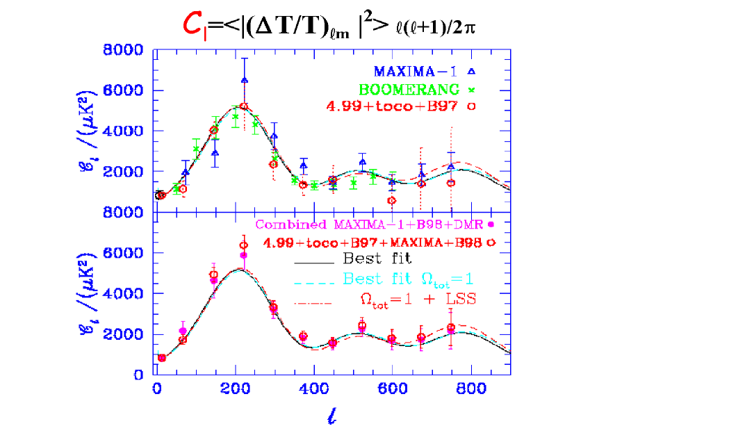
Figure 1.: The top figure shows ${\cal C}_{\ell}$ grouped in bandpowers for Boomerang-LDB (crosses), Maxima-I (triangles) and prior-CMB experiments (TOCO+Boomerang-NA+”April 99”, squares). The lower panel contrasts the optimally-combined power spectra for Boomerang+Maxima+DMR (squares) with that for Boomerang+Maxima+prior-CMB (circles), showing the prior experiments do not move ${\cal C}_{\ell}$ very much. Best-fit models for arbitrary $\Omega_{tot}$ and for $\Omega_{tot}$=1 are shown in both panels. The Boomerang 150A GHz map (i.e., for one of 16 bolometers) and the multifrequency Wiener-filtered Maxima-I map, its 124 square degrees drawn to scale, are shown in the bottom figure. Only the 440 square degrees within the central rectangle of the entire 1800 square degrees covered by Boomerang were used in the analysis.

We are only at the beginning of the high precision CMB era for primary anisotropies heralded by the arrival of Boomerang and Maxima, with interferometers taking data (VSA, CBI, DASI), the single dish ACBAR about to, and new LDBs to fly in the next few years (Arkeops, Tophat, Beast/Boost), as well as Boomerang-2001 and the neo-Maxima Maxipol, both concentrating on polarization. In April 2001, NASA’s HEMT-based MAP satellite will launch, with $12^{\prime}$ resolution, and in 2007, ESA’s bolometer+HEMT-based Planck satellite is scheduled for launch, with $5^{\prime}$ resolution.

The CMB Analysis Pipeline: Analyzing Boomerang and other experiments involves a pipeline that takes (1) the timestream in each of the bolometer channels coming from the balloon plus information on where it is pointing and turns it into (2) spatial maps for each frequency characterized by average temperature fluctuation values in each pixel (Fig. 1) and a pixel-pixel correlation matrix characterizing the noise, from which various statistical quantities are derived, in particular (3) the temperature power spectrum as a function of multipole (Fig. 1), grouped into bands, and two band-band error matrices which together determine the full likelihood distribution of the bandpowers (Bond, Jaffe & Knox 1998 [BJK98], BJK00). Fundamental to the first step is the extraction of the sky signal from the noise, using the only information we have, the pointing matrix mapping a bit in time onto a pixel position on the sky. To compare the data with millions of cosmological models, as we wish to do here, the radical compression step from 2 to 3 is essential, and hinges upon an accurate representation of the likelihood surface.

There is generally another step in between (2) and (3), namely separating the multifrequency spatial maps into the physical components on the sky: the primary CMB, the thermal and kinematic Sunyaev-Zeldovich effects, the dust, synchrotron and bremsstrahlung Galactic signals, the extragalactic radio and submillimetre sources. The strong agreement among the Boomerang maps indicates that to first order we can ignore this step, but it has to be taken into account as the precision increases. The Fig. 1 map is consistent with a Gaussian distribution, thus fully characterized by just the power spectrum. Higher order (concentration) statistics (3,4-point functions, etc.) tell us of non-Gaussian aspects, necessarily expected from the Galactic foreground and extragalactic source signals, but possible even in the early Universe fluctuations. For example, though non-Gaussianity occurs only in the more baroque inflation models of quantum noise, it is a necessary outcome of defect-driven models of structure formation. (Peaks compatible with Fig. 1 do not appear in non-baroque defect models, which now appear unlikely.) Though great strides have been made in the analysis of Boomerang and Maxima, there is intense needed effort worldwide now to develop new fast algorithms to deal with the looming megapixel datasets of LDBs and the satellites (e.g., Bond et al. 1999, Szapudi et al. 2000).

2. Cosmic Parameters

Parameters of Structure Formation: We usually adopt the restricted set of 7 cosmological parameters used in Let00 and Jet00, $\{\Omega_{\Lambda},\Omega_{k},\omega_{b},\omega_{cdm},n_{s},\tau_{C},\sigma_{8}\}$. The curvature energy is $\Omega_{k}\equiv 1-\Omega_{tot}$. The dark energy parameterized here by $\Omega_{\Lambda}$ could have complex dynamics associated with it, e.g., if it is the energy density of a scalar field which dominates at late times (now often termed a quintessence field, $Q$, with energy $\Omega_{Q}$, e.g., Steinhardt 2000). One popular phenomenology is to add one more parameter, $w_{Q}=p_{Q}/\rho_{Q}$, where $p_{Q}$ and $\rho_{Q}$ are the pressure and density of the $Q$-field. Thus $w_{Q}=-1$ and $\Omega_{Q}=\Omega_{\Lambda}$ for the cosmological constant. We have also allowed $w_{Q}$ to float.

We use 2 parameters to characterize the early universe primordial power spectrum of gravitational potential fluctuations $\Phi$, one giving the overall power spectrum amplitude ${\cal P}_{\Phi}(k_{n})$, and one defining the shape, a spectral tilt $n_{s}(k_{n})\equiv 1+d\ln{\cal P}_{\Phi}/d\ln k$, both at some (comoving) normalization wavenumber $k_{n}$. We really need another 2, ${\cal P}_{GW}(k_{n})$ and $n_{t}(k_{n})$, associated with the gravitational wave component. In inflation, the amplitude ratio is related to $n_{t}$ to lowest order, with ${\cal O}(n_{s}-n_{t})$ corrections at higher order, e.g., B96. There are also useful limiting cases for the $n_{s}-n_{t}$ relation. However, as one allows the baroqueness of the inflation models to increase, one can entertain a plethora of power spectra (with fully $k$-dependent $n_{s}(k)$ and $n_{t}(k)$) if one is artful enough in designing inflaton potential surfaces. As well, one can have more types of modes present, e.g., scalar isocurvature modes (${\cal P}_{is}(k_{n}),n_{is}(k)$) in addition to, or in place of, the scalar curvature modes (${\cal P}_{\Phi}(k_{n}),n_{s}(k)$). However, our philosophy is consider minimal models first, then see how progressive relaxation of the constraints on the inflation models, at the expense of increasing baroqueness, causes the parameter errors to open up. For example, with COBE-DMR and Boomerang, we can probe the GW contribution, but the data are not powerful enough to determine much. Planck can in principle probe the gravity wave contribution reasonably well.

We use another 2 parameters to characterize the transport of the radiation through the era of photon decoupling, which is sensitive to the physical density of the various species of particles present then, $\omega_{j}\equiv\Omega_{j}{\rm h}^{2}$. We really need 4: $\omega_{b}$ for the baryons, $\omega_{cdm}$ for the cold dark matter, $\omega_{hdm}$ for the hot dark matter (massive but light neutrinos), and $\omega_{er}$ for the relativistic particles present at that time (photons, very light neutrinos, and possibly weakly interacting products of late time particle decays). For simplicity, though, we restrict ourselves to the conventional 3 species of relativistic neutrinos plus photons, with $\omega_{er}$ therefore fixed by the CMB temperature and the relationship between the neutrino and photon temperatures determined by the extra photon entropy accompanying $e^{+}e^{-}$ annihilation. Of particular importance for the pattern of the radiation is the (comoving) distance sound can have influenced by recombination (at redshift $z_{r}=a_{r}^{-1}-1$),

$$r_{s}={6000\over\sqrt{3}}{\rm~{}Mpc}\int_{0}^{\sqrt{a_{r}}}{d\sqrt{a}\over(\omega_{m}+\omega_{er}a^{-1})^{1/2}(1+\omega_{b}a/(4\omega_{\gamma}/3))^{1/2}}\ ,$$ (1)

where $\omega_{\gamma}=2.46\times 10^{-5}$ is the photon density, $\omega_{er}=1.68\omega_{\gamma}$ for 3 species of massless neutrinos and $\omega_{m}\equiv\omega_{hdm}+\omega_{cdm}+\omega_{b}$.

The angular diameter distance is

$${\cal R}=\{d_{k}{\rm sinh}(\chi_{r}/d_{k}),\chi_{r},d_{k}{\rm sin}(\chi_{r}/d_{k})\},{\rm where}\,d_{k}={3000\over\sqrt{|\omega_{k}|}}{\rm~{}Mpc}\,,$$ (2)

$$\chi_{r}=6000{\rm~{}Mpc}\int_{\sqrt{a_{r}}}^{1}{d\sqrt{a}\over(\omega_{m}+\omega_{Q}a^{-6w_{Q}}+\omega_{k}a)^{1/2}}\,.$$

The 3 cases are for negative, zero and positive mean curvature, $d_{k}$ is the curvature scale and $\chi_{r}$ is the comoving distance to recombination. The location of the first acoustic peak, $L_{Pk}\approx 0.746\pi{\cal R}/r_{s}$ (e.g., Efstathiou and Bond 1999, hereafter EB99), depends upon $\omega_{b}$ through the sound speed as well as on $\omega_{k}$, $\omega_{\Lambda}$ and $\omega_{m}$. Thus $L_{Pk}$ defines a functional relationship among these parameters, a degeneracy (EB99) that would be exact except for the integrated Sachs-Wolfe effect, associated with the change of $\Phi$ with time if $\Omega_{\Lambda}$ or $\Omega_{k}$ is nonzero.

Our 7th parameter is an astrophysical one, the Compton ”optical depth” $\tau_{C}$ from a reionization redshift $z_{reh}$ to the present. It lowers ${\cal C}_{\ell}$ by $\exp(-2\tau_{C})$ at the high $\ell$’s probed by Boomerang. For typical models of hierarchical structure formation, we expect $\tau_{C}\mathrel{\hbox to0.0pt{\lower 3.0pt\hbox{$\mathchar 536\relax$}\hss}\raise 2.0pt\hbox{$\mathchar 316\relax$}}0.2$. It is partly degenerate with $\sigma_{8}$ and cannot be determined at this precision by CMB data now.

The LSS also depends upon our parameter set. Here we use a set of (relatively weak) constraints on $\ln\sigma_{8}^{2}$ from cluster abundance data and on $\Gamma+(n_{s}-1)/2$ from galaxy clustering data (B96, Let00). $\sigma_{8}^{2}$ is a bandpower for density fluctuations on a scale associated with rare clusters of galaxies, $8{\,{\rm h}^{-1}~{}\rm Mpc}$, which we often use in place of ${\cal P}_{\Phi}(k_{n})$ or ${\cal C}_{10}$ for the amplitude parameter. The mass-density-power-spectrum-shape-parameter $\Gamma$ depends upon $\{\omega_{m},\omega_{er},\omega_{b},{\rm h}\}$ and is related to the horizon scale when the energy density in relativistic particles equals that in nonrelativistic ones.

When we allow for freedom in $\omega_{er}$, the abundance of primordial helium, tilts of tilts ($dn_{\{s,is,t\}}(k_{n})/d\ln k,...$) for 3 types of perturbations, the parameter count would be 17, and many more if we open up full theoretical freedom in spectral shapes. However, as we shall see, as of now only 3 or 4 combinations can be determined with 10% accuracy with the CMB. Thus choosing 7 is adequate for the present, 6 of which are discretely sampled, with generous boundaries. For drawing cosmological conclusions we adopt a weak prior probability on the Hubble parameter and age: we restrict ${\rm h}$ to lie in the 0.45 to 0.9 range, and the age to be above 10 Gyr.

The First Peak, $\Omega_{tot}$ and $\Omega_{\Lambda}$: $L_{Pk}$ and its errors are found from the average and variance of $\ln L_{Pk}$, taken wrt the full probability function over our database described above (restricted for this exercise to the $\tau_{C}=0$ part and with the weak prior). As more CMB data were added, $L_{Pk}$ evolved and the errors shrunk considerably: $240^{+70}_{-54}$ for April 99 data, $220^{+30}_{-27}$ for TOCO+4.99 data, $224^{+23}_{-21}$ when Boomerang-NA was added, and $212^{+7}_{-7}$ when Boomerang-LDB and Maxima-1 were added to prior-CMB. The latter contrasts with $202^{+7}_{-7}$ for Boomerang-LDB alone, $226^{+17}_{-16}$ for Maxima-1 alone, and $208^{+7}_{-7}$ for the combination. The numbers change a bit depending upon exactly what prior one chooses or what functional forms one averages over. For the choice here, although there is a large difference in the mean between the Maxima and Boomerang numbers, it is not unreasonable within the errors. Other ways of doing this make the discrepancy seem more statistically significant (e.g., Page 2000, these proceedings).

In Fig. 2, we show the lines of constant $L_{Pk}\propto{\cal R}/r_{s}$ in the $\Omega_{tot}$–$\Omega_{\Lambda}$ plane, for given $\omega_{m}$ and $\omega_{b}$, using the formulas given above and discussed in more detail in EB99. The $\pm 10$ band around 210 corresponds to our best $L_{Pk}$ estimate of $212\pm 7$ using all current CMB data. Note that the constant $L_{Pk}$ lines look rather similar to the contours shown in the right panel, showing that the ${\cal R}/r_{s}$ degeneracy plays a large role in determining the contours. The contours hug the $\Omega_{tot}=1$ line more closely than the allowed $L_{Pk}$ band does for the maximum probability values of $\omega_{m}$ and $\omega_{b}$, because of the shift in the allowed $L_{Pk}$ band as $\omega_{m}$ and $\omega_{b}$ vary in this plane. See also Bond et al. (2001b, [capp2K]) for $L_{Pk}$ plots in the quintessence plane, $w_{Q}$-$\Omega_{Q}$, which demonstrate why $w_{Q}$ is poorly determined by CMB alone.

Table 1.: Cosmological parameter values and their 1-sigma errors are shown, determined after marginalizing over the other $6$ cosmological and $4^{+}$ experimental parameters, for B98+Maxima-I+prior-CMB and the weak prior, $0.45\mathrel{\hbox to0.0pt{\lower 3.0pt\hbox{$-$}\hss}\raise 2.0pt\hbox{$\mathchar 316\relax$}}{\rm h}\mathrel{\hbox to0.0pt{\lower 3.0pt\hbox{$-$}\hss}\raise 2.0pt\hbox{$\mathchar 316\relax$}}0.9$, age $>10$ Gyr. The LSS prior was also designed to be weak. In the first set $\Omega_{tot}$ varies, in the second set it is fixed to unity. Similar tables for B98+DMR are given in Let00 and for B98+MAXIMA-I+DMR in Jet00. We have set the quintessence $w_{Q}=p_{Q}/\rho_{Q}$ parameter to $-1$, the cosmological constant case, but the last line shows the limit on $w_{Q}$ if we allow it to vary (the other parameters do not move much). SN1 results on $w_{Q}$ with earlier CMB data were given in Perlmutter et al. (1999). The detections in the table are clearly very stable if extra ”prior” probabilities for LSS and SN1 are included, and are also stable with much stronger priors on ${\rm h}$, but do move if the BBN-derived $0.019\pm 0.002$ prior is imposed. If $\Omega_{tot}$ is varied, parameters derived from our basic 7 come out to be: age=$13.2\pm 1.3$ Gyr, ${\rm h}=0.70\pm 0.09$, $\Omega_{m}=0.35\pm.06$, $\Omega_{b}=0.065\pm.019$. Restriction to $\Omega_{tot}=1$ yields: age=$11.6\pm 0.4$ Gyr, ${\rm h}=0.80\pm.04$, $\Omega_{m}=0.31\pm.03$, $\Omega_{b}=0.046\pm.005$.

	cmb	+LSS	+SN1	+SN1+LSS
$\Omega_{tot}$	$1.09^{+.07}_{-.07}$	$1.08^{+.06}_{-.06}$	$1.04^{+.06}_{-.05}$	$1.04^{+.05}_{-.04}$
$\Omega_{b}{\rm h}^{2}$	$.031^{+.005}_{-.005}$	$.031^{+.005}_{-.005}$	$.031^{+.005}_{-.005}$	$.031^{+.005}_{-.005}$
$\Omega_{cdm}{\rm h}^{2}$	$.17^{+.06}_{-.05}$	$.14^{+.03}_{-.02}$	$.13^{+.05}_{-.05}$	$.15^{+.03}_{-.02}$
$n_{s}$	$1.05^{+.09}_{-.08}$	$1.04^{+.09}_{-.08}$	$1.05^{+.10}_{-.09}$	$1.06^{+.08}_{-.08}$
$\Omega_{\Lambda}$	$0.48^{+.20}_{-.26}$	$0.63^{+.08}_{-.09}$	$0.72^{+.07}_{-.07}$	$0.70^{+.04}_{-.05}$
	$\Omega_{tot}$	=1	CASE	($w_{Q}$=-1)
$\Omega_{b}{\rm h}^{2}$	$.030^{+.004}_{-.004}$	$.030^{+.003}_{-.004}$	$.030^{+.004}_{-.004}$	$.030^{+.003}_{-.004}$
$\Omega_{cdm}{\rm h}^{2}$	$.19^{+.06}_{-.05}$	$.17^{+.02}_{-.02}$	$.16^{+.03}_{-.03}$	$.17^{+.01}_{-.02}$
$n_{s}$	$1.02^{+.08}_{-.07}$	$1.03^{+.08}_{-.07}$	$1.03^{+.08}_{-.07}$	$1.04^{+.07}_{-.07}$
$\Omega_{\Lambda}$	$0.58^{+.17}_{-.27}$	$0.66^{+.04}_{-.06}$	$0.71^{+.06}_{-.07}$	$0.69^{+.03}_{-.05}$
$w_{Q}$ (95%)	$<-0.29$	$<-0.33$	$<-0.69$	$<-0.73$

Figure 2.: The top panels show 1,2,3-sigma likelihood contours for the weak-H+age prior probability (right) and when the LSS ”prior” is included (left). In the right panel, ”prior-CMB” experiments (TOCO+Boomerang-NA+”April 99”) were included instead of just DMR, but the figure is very similar for Boomerang+Maxima+DMR. The supernova contours are also plotted, and the solid contour lines are what you get when you combine the two likelihoods. The bottom panels show lines of constant $L_{Pk}$ in the $\Omega_{m}$–$\Omega_{\Lambda}$ plane for two choices of $\{\omega_{m},\omega_{b}\}$, left the most probable values, right when the current BBN constraint is imposed (lowering $\omega_{b}$ increases the sound speed, decreasing $L_{Pk}$, and varying $\omega_{m}$ also shifts it). The $0.65<{\rm h}<0.75$ (heavier shading, $H_{0}$) and $11<$ age $<15$ (lighter shading, $t_{0}$) ranges and decelerations $q_{0}=0,-1/3,-1/2$ are also noted. The sweeping back of the $L_{Pk}$ curves into the closed models as $\Omega_{\Lambda}$ is lowered shows that even if $\Omega_{tot}$=1 is the correct answer, the phase space results in a 1D projection onto the $\Omega_{tot}$ axis that would be skewed to $\Omega_{tot}>1$, a situation we see in Table 1. Note that the contours in the top left panel are near the diagonal $\Omega_{tot}=1$ line, but also follow a weighted average of $L_{Pk}\sim 210$ lines. This approximate degeneracy implies $\Omega_{\Lambda}$ is poorly constrained for CMB-only, but it is broken when LSS is added, giving a solid SN1-independent $\Omega_{\Lambda}$ ”detection”. $L_{Pk}$ and contour plots in the $w_{Q}$–$\Omega_{Q}$ plane for $\Omega_{tot}$=1 are given in capp2K.

Marginalized Estimates of our Basic 7 Parameters: Table 1 shows there are strong detections with only the CMB data for $\Omega_{tot}$, $\omega_{b}$ and $n_{s}$ in the minimal inflation-based 7 parameter set, and a reasonable detection of $\omega_{cdm}$. The ranges quoted are Bayesian 50% values and the errors are 1-sigma, obtained after projecting (marginalizing) over all other parameters. That $\Omega_{\Lambda}$ is not well determined is a manifestation of the $\Omega_{tot}$–$\Omega_{\Lambda}$ near-degeneracy discussed above, which is broken when LSS is added because the CMB-normalized $\sigma_{8}$ is quite different for open cf. $\Lambda$ models. Supernova at high redshift give complementary information to the CMB, but with CMB+LSS (and the inflation-based paradigm) we do not need it: the CMB+SN1 and CMB+LSS numbers are quite compatible. In our space, the Hubble parameter, ${\rm h}=(\sum_{j}(\Omega_{j}{\rm h}^{2}))^{1/2}$, and the age of the Universe, $t_{0}$, are derived functions of the $\Omega_{j}{\rm h}^{2}$: representative values are given in the Table caption.

Fig. 3 shows how the parameter estimations evolved as more CMB data were added (for the weak+LSS prior). With just the COBE-DMR+LSS data, the 2-sigma contours were already localized in $\omega_{cdm}$. Without LSS, it took the addition of Maxima-1 before it began to localize. $\Omega_{k}$ localized near zero when TOCO was added to the April 99 data, more so when Boomerang-NA was added, and much more so when Boomerang-LDB and Maxima-1 were added. Some $n_{s}$ localization occurred with just ”prior-CMB” data. $\omega_{b}$ really focussed in with Boomerang-LDB and Maxima-1, as did $\Omega_{\Lambda}$.

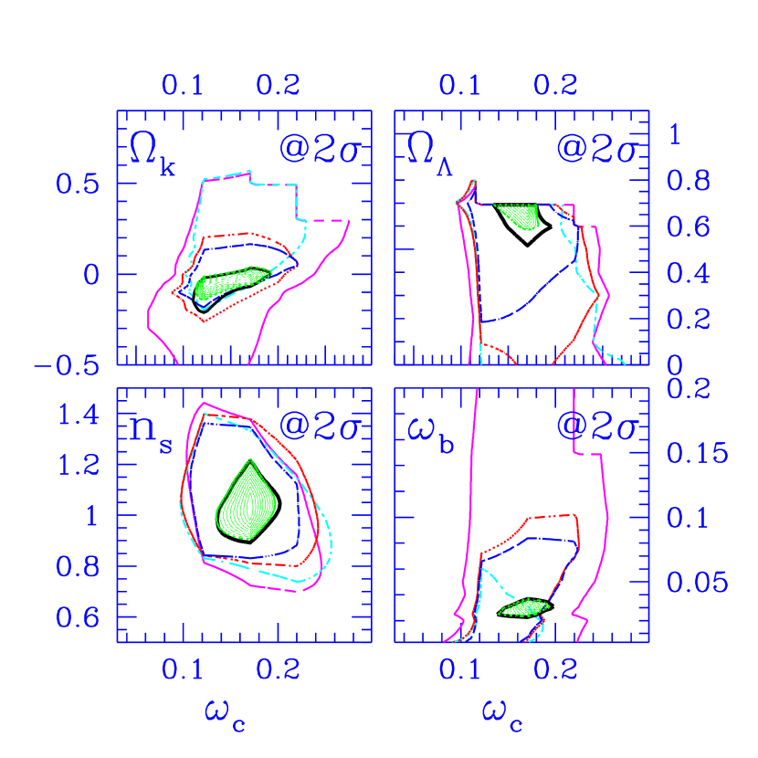
Figure 3.: 2-sigma likelihood contours for the dark matter density $\omega_{c}=\Omega_{cdm}{\rm h}^{2}$ and $\{\Omega_{k},\Omega_{\Lambda},n_{s},\omega_{b}\}$ are plotted for LSS, the weak-H+age cosmological prior, and the following CMB experimental combinations: DMR (short-dash); the ”April 99” data (short-dash long-dash); TOCO+4.99 data (dot short-dash); Boomerang-NA+TOCO+4.99 data (dot long-dash, termed ”prior-CMB”); Boomerang-LDB+Maxima-1+Boomerang-NA+TOCO+4.99 data (heavy solid, all-CMB). These $2\sigma$ lines tend to go from outside to inside as more CMB experiments are added. The smallest 2-sigma region (dotted and interior) shows SN1+LSS+all-CMB, when SNI data is added. For the $\Omega_{\Lambda}$, $n_{s}$ and $\omega_{b}$ plots , $\Omega_{tot}$=1 has been assumed, but the values do not change that much if $\Omega_{tot}$ floats, as Table 1 shows for all-CMB. (The discreteness of the ${\cal C}_{\ell}$–database is responsible for the sharpness of the contour edges, especially evident in the $\omega_{c}$–$\Omega_{\Lambda}$ CMB+LSS case. Though different interpolation schemes can round these off somewhat, it is the price of our finite grid.)

We have also considered what happens as we let $\Omega_{m\nu}/\Omega_{m}$, the fraction of the matter in massive neutrinos, vary from 0 to 0.3, for LSS + all of the CMB data and $\Omega_{tot}$=1 (Bond et al. 2001a, [$\nu$2K]). Until Planck precision, the CMB data by itself will not be able to strongly discriminate this ratio. Adding HDM does have a strong impact on the CMB-normalized $\sigma_{8}$ and the shape of the density power spectrum (effective $\Gamma$ parameter), both of which mean that when LSS is included, adding some HDM to CDM is strongly preferred in the absence of $\Omega_{\Lambda}$. However, though higher $\Omega_{m}$ is preferred at the expense of less dark energy, significant $\Omega_{\Lambda}$ is still required (see $\nu$2K for the evolution of the CMB+LSS 2-sigma contours in the $(\omega_{hdm}+\omega_{cdm})$–$\Omega_{\Lambda}$ plane as $\Omega_{m\nu}/\Omega_{m}$ is varied). The $\omega_{b}$ and $n_{s}$ likelihood curves are essentially independent of $\Omega_{m\nu}/\Omega_{m}$.

The Future, Forecasts for Parameter Eigenmodes: We can also forecast dramatically improved precision with further analysis of Boomerang and Maxima, future LDBs, MAP and Planck. Because there are correlations among the physical variables we wish to determine, including a number of near-degeneracies beyond that for $\Omega_{tot}$–$\Omega_{\Lambda}$ (EB99), it is useful to disentangle them, by making combinations which diagonalize the error correlation matrix, ”parameter eigenmodes” (e.g., B96, EB99). For this exercise, we will add $\omega_{hdm}$ and $n_{t}$ to our parameter mix, but set $w_{Q}$=$-1$, making 9. (The ratio ${\cal P}_{GW}(k_{n})/{\cal P}_{\Phi}(k_{n})$ is treated as fixed by $n_{t}$, a reasonably accurate inflation theory result.) The forecast for Boomerang+DMR based on the 440 square degree patch with a single 150 GHz bolometer used in the published data is 3 out of 9 linear combinations should be determined to $\pm 0.1$ accuracy. This is indeed what we get in the full analysis of Let00 for CMB only. If 4 of the 6 150 GHz channels are used and the region is doubled in size, we predict 4/9 could be determined to $\pm 0.1$ accuracy. The Boomerang team is still working on the data to realize this promise. And if the optimistic case for all the proposed LDBs is assumed, 6/9 parameter combinations could be determined to $\pm 0.1$ accuracy, 2/9 to $\pm 0.01$ accuracy. The situation improves for the satellite experiments: for MAP, we forecast 6/9 combos to $\pm 0.1$ accuracy, 3/9 to $\pm 0.01$ accuracy; for Planck, 7/9 to $\pm 0.1$ accuracy, 5/9 to $\pm 0.01$ accuracy. While we can expect systematic errors to loom as the real arbiter of accuracy, the clear forecast is for a very rosy decade of high precision CMB cosmology that we are now fully into.

References

- Bond 1996 Bond, J.R. 1996, in Cosmology and Large Scale Structure, Les Houches Session LX, eds. R. Schaeffer et al. (Elsevier), p. 469 [B96]
- Bond et al. 1999 Bond, J.R., Crittenden, R., Jaffe, A.H. & Knox, L. 1999, Computing in Science and Engineering 1, 21, astro-ph/9903166, and references therein.
- Bond, Jaffe, & Knox 1998 Bond, J.R., Jaffe, A.H. & Knox, L. 1998, PRD 57, 2117, astro-ph/9708203 [BJK98]
- Bond, Jaffe, & Knox 2000 Bond, J.R., Jaffe, A.H. & Knox, L. 2000, ApJ 533, 19, astro-ph/9808264 [BJK00]
- Bond et al. 2001a Bond, J.R., Pogosyan, D., Prunet, S. & the MaxiBoom Collaboration 2001a, Proc. Neutrino 2000, ed. Law, J., Simpson, J. (Elsevier) [2K]
- Bond et al. 2001b Bond, J.R., Pogosyan, D., Prunet, S., Sigurdson, K. & the MaxiBoom Collaboration 2001b, Proc. CAPP-2000, ed. R. Durrer, J. Garcia-Bellida, M. Shaposhnikov (AIP) [capp2K]
- deBernardis et al. 2000 de Bernardis, P. et al. 2000, Nature 404, 995, astro-ph/00050087; 2001, these proceedings; http://www.physics.ucsb.edu/boomerang/ [Boomerang-LDB]
- Efstathiou & Bond 1999 Efstathiou, G. & Bond, J.R. 1999, Mon. Not. R. Astron. Soc. 304, 75, where many other near-degeneracies between cosmological parameters are also discussed. [EB99]
- Hanany et al. 2000 Hanany, S. et al. 2000, ApJ Lett., submitted, astro-ph/0005123; http://cfpa.berkeley.edu/maxima [MAXIMA-1]
- Jaffe et al. 2000 Jaffe, A. et al. 2000, PRL, in press, astro-ph/0007333 [Jet00]
- Lange et al. 2000 Lange, A. et al. 2000, PRD, in press, astro-ph/0005004 [Let00]
- Mauskopf et al. 2000 Mauskopf, P. et al., 2000, ApJ Lett 536, L59 [Boomerang-NA]
- Miller et al. 1999 Miller, A.D. et al., 1999, ApJ Lett 524, L1 [TOCO]
- Perlmutter et al. 1999 Perlmutter, S., Turner, M. & White, M. 1999, PRL 83, 670, from which the – SN1 likelihood function was taken, courtesy of Saul Perlmutter; see also Wang, L. et al., astro-ph/9901388
- 1 Steinhardt, P. 2000, http://feynman.princeton.edu/steinh/ ”Quintessence? - an overview”, gives a pedagogical introduction, and references.
- Szapudi et al. 2000 Szapudi, I., Prunet, S., Pogosyan, D., Szalay, A. & Bond, J.R. 2000, ApJ Lett, in press, astro-ph/0010256 and references therein.