Not enough stellar mass Machos in the Galactic halo

Abstract

We present an update of results from the search for microlensing towards the Large Magellanic Cloud (lmc) by eros (Expérience de Recherche d’Objets Sombres). We have now monitored 25 million stars over three years. Because of the small number of observed microlensing candidates (four), our results are best presented as upper limits on the amount of dark compact objects in the halo of our Galaxy. We discuss critically the candidates and the possible location of the lenses, halo or lmc. We compare our results to those of the macho group. Finally, we combine these new results with those from our search towards the Small Magellanic Cloud as well as earlier ones from the eros1 phase of our survey. The combined data is sensitive to compact objects in the broad mass range $10^{-7}-10\,{\rm M}_{\odot}$. The derived upper limit on the abundance of stellar mass machos rules out such objects as the dominant component of the Galactic halo if their mass is smaller than $2{\rm M}_{\odot}$.

1 Research context

The search for gravitational microlensing in our Galaxy has been going on for a decade, following the proposal to use this effect as a probe of the dark matter content of the Galactic halo [1]. The first microlensing candidates were reported in 1993, towards the lmc [2, 3] and the Galactic Centre [4] by the eros, macho and ogle collaborations.

Because they observed no microlensing candidate with a duration shorter than 10 days, the eros1 and macho groups were able to exclude the possibility that more than 10% of the Galactic dark matter resides in planet-sized objects [5, 6, 7, 8, 9].

However a few events were detected with longer timescales. In their two-year analysis [10], the macho group estimated, from 6-8 candidate events towards the lmc, an optical depth of order half that required to account for the dynamical mass of a “standard” spherical dark halo; the typical Einstein radius crossing time of the events, $t_{E}$, implied an average mass of about 0.5 M_⊙ for halo lenses [10]. Based on two candidates, eros1 set an upper limit on the halo mass fraction in objects of similar masses [11, 7], that is below that required to explain the rotation curve of our Galaxy.

The second phase of the eros programme was started in 1996, with a ten-fold increase over eros1 in the number of monitored stars in the Magellanic Clouds. The analysis of the first two years of data towards the Small Magellanic Cloud (smc) allowed the observation of one microlensing event [12] also detected by [13]. This single event, out of 5.3 million monitored stars, allowed eros2 to further constrain the halo composition, excluding in particular that more than 50 % of the standard dark halo is made up of $0.01-0.5\>{\rm M}_{\odot}$ objects [14]. In contrast, an optical detection of a halo white dwarf population was reported [15], compatible with a galactic halo full of white dwarfs.

Very recently, the macho group presented an analysis of 5.7 year light curves of 10.7 million stars in the lmc [16] with an improved determination of their detection efficiency and a better rejection of background supernova explosions behind the lmc. They now favour a galactic halo macho component of 20% in the form of 0.4 M_⊙ objects. Within a few days, the detection of a halo white dwarf population at the level of a 10% component was also reported by [17]. Simultaneously, the eros2 group presented its results from a two-year survey of 17.5 million stars in the lmc [18]. One eros1 microlensing candidate, eros1-lmc-2, was seen to vary again, 8 years after its first brightening, and was thus eliminated from the list of microlensing candidates. Two new candidates were identified (eros2-lmc-3 and 4). Because this is much lower than expected if machos are a substantial component of the galactic halo, and because these two new candidates do not show excellent agreement with simple microlensing light curves, eros chose to combine these results with those from previous eros analyses, and to quote an upper limit on the fraction of the galactic halo in the form of machos.

In this article, we describe an update on the eros2 lmc data, an analysis of the three-year light curves from 25.5 million stars. While the sensitivity is improved, the main conclusions are unchanged compared to [18]. One of the two-year candidates was seen to vary in the third season and was thus rejected. Three new candidates have been detected. We combine these eros2 lmc results with those of previous independent eros analyses, and derive the strongest limit obtained thus far on the amount of stellar mass objects in the Galactic halo.

2 Experimental setup and LMC observations

The telescope, camera, telescope operation and data reduction are as described in [19, 12]. Since August 1996, we have been monitoring 66 one square-degree fields in the lmc, simultaneously in two wide passbands. Of these, data prior to May 1999 from 39 square-degrees spread over 64 fields have been analysed. In this period, two thirds of the fields were imaged about 210 times in average; the remaining third were imaged only about 110 times. The exposure times range from 3 min in the lmc center to 12 min on the periphery; the average sampling is once every 4 days (resp. 8 days).

3 LMC data analysis

The analysis of the lmc data set was done using a program independent from that used in the smc study, with largely different selection criteria. The aim is to cross-validate both programs (as was already done in the analysis of eros1 Schmidt photographic plates [11]) and avoid losing rare microlensing events. The analysis is very similar to that reported in [18]. We only give here a list of the various steps, as well as a short description of the differences with respect to our two-year analysis. A detailed description of the analysis will be provided in [20, 21].

We first select the 6% “most variable” light curves, a sample much larger than the number of detectable variable stars. This subset of our data is “enriched” in genuine variable stars, but also and mainly in photometrically biased light curves, i.e. those of stars especially sensitive to the observing conditions, such as stars very close to nebulosities or to bright stars. Working from this “enriched” subset, we apply a first set of cuts to select, in each colour separately, the light curves that exhibit significant variations. We first identify the baseline flux in the light curve - basically the most probable flux. We then search for runs along the light curve, i.e. groups of consecutive measurements that are all on the same side of the baseline flux. We select light curves that either have an abnormally low number of runs over the whole light curve, or show one long run (at least 5 valid measurements) that is very unlikely to be a statistical fluctuation. We then discard light curves with a low signal-to-noise ratio by requiring that the group of 5 most luminous consecutive measurements be significantly further from the baseline than the average spread of the measurements. We also check that the measurements inside the most significant run show a smooth time variation.

The second set of cuts compares the measurements with the best fit point-lens point-source constant speed microlensing light curve (hereafter “simple microlensing”). They allow us to reject variable stars whose light curves differ too much from simple microlensing, and are sufficiently loose not to reject light curves affected by blending, parallax or the finite size of the source, and most cases of multiple lenses or sources. We also require that the fitted time of maximum magnification lie within the observing period or very close to it, and that the fitted timescale is shorter than 300 days. The latter cut is equivalent to requiring that the baseline flux of the star is observed for at least a few months; this is necessary in any analysis using this baseline flux. At this stage of the analysis, all cuts have been applied independently in the two passbands.

After this second set of cuts, stars selected separately in the two passbands represent about 0.01% of the initial sample; almost all of them are found in two thinly populated zones of the colour-magnitude diagram. The third set of cuts deals with this physical background. The first zone contains stars brighter and much redder than those of the red clump; variable stars in this zone are rejected if they vary by less than a factor two or have a very poor fit to simple microlensing. The second zone is the top of the main sequence, where the selected stars, known as blue bumpers [10], display variations that are almost always smaller than 60% of the base flux or at least 20% lower in the visible passband than in the red one. These cannot correspond to simple microlensing, which is achromatic; neither can they correspond to microlensing plus blending with another unmagnified star, as it would imply blending by even bluer stars, which is very unlikely. We thus reject all candidates from the second zone exhibiting one of these two features (see Fig. 1).

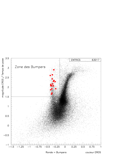
Figure 1: A colour-magnitude diagram in one eros field, showing the location of candidates identified as “blue bumpers”, either from their small amplitude, or from their chromatic variation (larger in the red than in the visible passband).

Compared to the analysis in [18], two new cuts are introduced to reject other types of variable stars that were not present in the two-year analysis. The first one is aimed at stars which have a roughly constant luminosity for some time, then vary typically over one or two months to reach a new constant level. We cannot yet conclude whether these are physical variable stars or some kind of instrumental problem. The second cut is aimed at novæ and supernovæ. It rejects light curves which have a rise time significantly smaller than the decline time; it is not applied to events with a timescale longer than 60 days, in order not to reject microlensing phenomena with parallax effects, that also show an asymmetry.

The final cuts are simply tighter cuts on the fit quality, applied to both colours (whereas similar previous cuts were applied independently in each passband), and a requirement that the observed magnification be at least 1.40 .

The tuning of each cut and the calculation of the microlensing detection efficiency are done with simulated simple microlensing light curves, as described in [12]. For the efficiency calculation, microlensing parameters are drawn as follows : time of maximum magnification $t_{0}$ uniformly within the observing period $\pm 150$ days, impact parameter normalised to the Einstein radius $u_{0}\in[0,2]$ uniformly, and timescale $t_{E}\in[1,400]$ days uniformly in $\ln(t_{E})$. All cuts on the data were also applied to the simulated light curves.

Figure 2: Light curves of candidates EROS-LMC-3 and 5 (visible passband). The plain curves show the best point-lens point-source fits; time is in days since Jan 1.0, 1990 (JD 2,447,892.5).

Figure 3: Same as Fig.2 for candidates EROS-LMC-6 and 7.

Only four candidates remain after all cuts. Of the two candidates presented in [18], eros2-lmc-3 is still a member of this list, while eros2-lmc-4 was seen to vary at least twice in the third season and was thus rejected. There are three new candidates, numbered 5 to 7. Their light curves are shown in Figs. 2 and 3; microlensing fit parameters are given in Table 1. Although the candidates pass all cuts, agreement with simple microlensing is not excellent. In particular, eros2-lmc-5 is dubious : it has a bad fit to simple microlensing and is located in an atypical region of the colour-magnitude diagram. The geometric mean of the candidates timescales is about 32 days, including that of the eros1 candidate lmc-1.

	$u_{0}$	$t_{E}$	$c_{\rm\,bl}^{R}$	$c_{\rm\,bl}^{V}$	$\chi^{2}/{\rm dof}$	$V_{J}$
lmc-3	$0.21$	$44$	$0.75$	1	219/143	22.4
lmc-5	$0.58$	$24$	$0.91$	1	658/176	19.2
lmc-6	$0.38$	$36$	$0.72$	1	682/411	21.3
lmc-7	$0.23$	$33$	$0.45$	1	722/356	22.7

Table 1: Results of microlensing fits to the four eros2 lmc candidates; $t_{E}$ is the Einstein radius crossing time in days, $u_{0}$ the impact parameter, and $c_{\rm\,bl}^{R(V)}$ the $R(V)$ blending coefficients, constrained to be smaller than unity.

The microlensing detection efficiency of this analysis, normalised to events with an impact parameter $u_{0}<1$ and to an observing period $T_{\rm obs}$ of three years, is summarised in Table 2. The main source of systematic error is the uncertainty in the influence of blending. Blending lowers the observed magnifications and timescales. While this decreases the efficiency for a given star, the effective number of monitored stars is increased so that there is partial compensation. This effect was studied with synthetic images using measured magnitude distributions [22]. Our final efficiency is within 10% of the “naive” sampling efficiency. Compared to the efficiency in [18], the present one is improved for the longest and shortest durations, but slightly lower for average durations around 50 days. This is largely explained by the fact that we have included in the present analysis stars in external lmc fields that were sampled less frequently.

$t_{E}$	6.3	13	28	40	90	175	250	360
$\epsilon$	2.7	6.7	11	14	19	22	17.5	2

Table 2: eros2 detection efficiency in % for the lmc 3-year analysis, as a function of the Einstein radius crossing time $t_{E}$ in days, normalised to events generated with $u_{0}<1$, and to $T_{\rm obs}=3{\rm\>yrs}$.

4 Limits on Galactic halo MACHOs

eros has observed six microlensing candidates towards the Magellanic Clouds, one from eros1 and four from eros2 towards the lmc, and one towards the smc. As discussed in [12], and further in [23], we consider that the long duration of the smc candidate together with the absence of any detectable parallax, in our data as well as in that of the macho group [13], indicates that it is most likely due to a lens in the smc. For that reason, the limit derived below uses the five lmc candidates. (The limit corresponding to all six candidates would be about a factor 1.13 times the limit shown, for masses larger than 0.01 solar mass.)

The limits on the contribution of dark compact objects to the Galactic halo are obtained by comparing the number and durations of microlensing candidates with those expected from Galactic halo models. We use here the so-called “standard” halo model described in [12] as model 1, but have checked that we obtain similar results for other reasonable halo models. The model predictions are computed for each eros data set in turn, taking into account the corresponding detection efficiencies ([11, 8, 14] and Table 2 above), and the four predictions are then summed. In this model, all dark objects have the same mass $M$; we have computed the model predictions for many trial masses $M$ in turn, in the range [$10^{-8}\>{\rm M}_{\odot}$, $10^{2}\>{\rm M}_{\odot}$].

The method used to compute the limit is as in [11]. We consider two ranges of timescale $t_{E}$, within or outside the interval I $=[7.5;190]$ days. This interval was chosen as follows. We first determine the average mass corresponding to the mean duration of the five lmc candidates, at about $0.2\>{\rm M}_{\odot}$. We then compute the expected distribution of microlensing timescales for this average mass and check that the observed spread in timescales for the candidates is compatible with the width of this distribution. This means that our candidates are compatible with the hypothesis that their spread in mass contributes very little to the width of the timescale distribution. The interval I is then chosen as a symmetrical interval in $\ln(t_{E})$ that contains 99% of the timescale distribution for halo machos of $0.2\>{\rm M}_{\odot}$. Of course, all five lmc candidates have timescales well within the interval I.

We can then compute, for each mass $M$ and any halo fraction $f$, the combined Poisson probability for obtaining, in the four different eros data sets taken as a whole, zero candidate outside I and five or less within I. For any value of $M$, the limit $f_{\rm max}$ is the value of $f$ for which this probability is 5%. Whereas the actual limit depends somewhat on the precise choice of I, the difference (smaller than 5%) is noticeable only for masses around 0.01 and $10\>{\rm M}_{\odot}$. Furthermore, we consider our choice for I to be a conservative one.

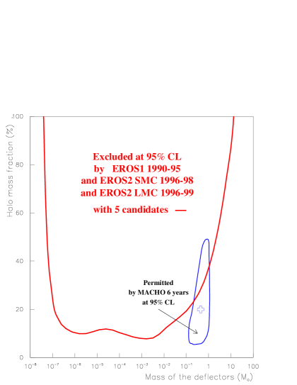
Figure 4: 95% C.L. exclusion diagram on the halo mass fraction in the form of compact objects of mass $M$, for the standard halo model ($4\times 10^{11}\>{\rm M}_{\odot}$ inside 50 kpc), from all lmc and smc eros data 1990-99. The solid line is the limit inferred from the five lmc microlensing candidates. The new macho 95% C.L. accepted region is the closed contour, with the preferred value indicated by the cross [16].

Figure 4 shows the 95% C.L. exclusion limit derived from this analysis on the halo mass fraction, $f$, for any given dark object mass, $M$. The solid line corresponds to the five lmc candidates; it is the main result of this article. This limit rules out a standard spherical halo model fully comprised of objects with any mass function inside the range $[10^{-7}-10]\;M_{\odot}$. In the region of stellar mass objects, where this result improves most on previous ones, the new lmc data contribute about 73% to our total sensitivity (the smc and eros1 lmc data contribute 10% and 17% respectively). The total sensitivity for $t_{E}=50$ days, that is proportional to the sum of $N_{*}\,T_{\rm obs}\,\epsilon(t_{E}=50{\rm d})$ over the four eros data sets, is about 3.2 times larger than that of [10] and two thirds that of [16].

5 Discussion

After nine years of monitoring the Magellanic Clouds, eros has a meager crop of five microlensing candidates towards the lmc and one towards the smc, whereas about 30 events are expected towards the lmc for a spherical halo fully comprised of $0.4\>{\rm M}_{\odot}$ objects. Moreover, some of the candidates cannot be considered excellent. These candidates were obtained from four different data sets analysed by independent, cross-validated programs. So, the small number of observed events is unlikely to be due to bad (and overestimated) detection efficiencies.

This allows us to put strong constraints on the fraction of the halo made of objects in the range [$10^{-7}\>{\rm M}_{\odot}$, $10\>{\rm M}_{\odot}$], excluding in particular at the 95% C.L. that more than 40% of the standard halo be made of objects with up to $1\>{\rm M}_{\odot}$. The preferred value quoted in [16], $f=0.2$ and $0.4\>{\rm M}_{\odot}$, is consistent with our limit as can be seen in Fig. 4. (The upper part - about 25% - of the domain allowed by [16] is excluded by the limit we report here.)

There are several differences which should be kept in mind while comparing the two experiments. First, eros uses less crowded fields than macho with the result that blending is relatively unimportant for eros. (Were eros results to be corrected for blending, the detection efficiency would increase slightly and the reported limit would be stronger.) Second, eros covers a larger solid angle (64 deg² in the lmc and 10 deg² in the smc) than macho, which monitors primarily 15 deg² in the central part of the lmc. The eros rate should thus be less contaminated by self-lensing, i.e. microlensing of lmc stars by dimmer lmc objects, which should be more common in the central regions. The importance of self-lensing was first stressed in [24, 25]. Third, the macho data have a more frequent time sampling.

The results from eros and macho are apparently consistent, but the way they are interpreted is different. macho reports a signal and considers the contamination of its sample as low or null. eros2 quotes an upper limit and does not claim its sample to be background-free. The position of the lenses along the line of sight, halo or Magellanic Clouds, is also an issue. macho has compared the spatial distribution of its candidates across the face of the lmc and observes a better agreement with the halo hypothesis than with a specific model of the lmc. On the other hand, because the eros stars are spread over a wider field, the fact that the eros sample corresponds to a lower central value of the event rate (about twice lower than that of macho) is compatible with an interpretation where a noteable fraction of the events are due to self-lensing. The small number of eros candidates precludes at present any definitive conclusion on that topic.

It seems likely that the single most important input to the question of the position of the lenses will come from the comparison of the microlens candidates samples towards the smc with those towards the lmc. Because the two lines of sight are rather close (about 20 degrees apart), the timescale distributions of microlensing candidates towards the two Clouds should be nearly identical if lenses belong to the galactic halo. Also, the event rates should be comparable, although the ratio is more halo model dependent. At present, eros has analysed two seasons of smc data [14] and macho has not yet presented its detection efficiency towards the smc. From the published eros efficiencies, and assuming that the macho efficiencies towards the smc are similar to those towards the lmc, it can be expected that the completed experiments will have gathered between five and ten microlenses towards the smc. This should allow a significant comparison of the timescales (see also the discussion in [23]).

Finally, let us mention that, given the scarcity of our candidates and the possibility that some observed microlenses actually lie in the Magellanic Clouds, eros is not willing at present to quote a non zero lower limit on the fraction of the Galactic halo comprised of dark compact objects with masses up to a few solar masses.

Acknowledgements We are grateful to D. Lacroix and the staff at the Observatoire de Haute Provence and to A. Baranne for their help with the MARLY telescope. The support by the technical staff at ESO, La Silla, is essential to our project. We thank J.F. Lecointe for assistance with the online computing. We thank all non-eros members who participated in data taking.

References

- [1] Paczyński B., 1986, ApJ 304, 1
- [2] Aubourg É. et al. (eros), 1993, Nat 365, 623
- [3] Alcock C. et al. (macho), 1993, Nat 365, 621
- [4] Udalski A. et al. (ogle), 1993, Acta Astron. 43, 289
- [5] Aubourg É. et al. (eros), 1995, A&A 301, 1
- [6] Alcock C. et al. (macho), 1996, ApJ 471, 774
- [7] Renault C. et al. (eros), 1997, A&A 324, L69
- [8] Renault C. et al. (eros), 1998, A&A 329, 522
- [9] Alcock C. et al. (macho + eros), 1998, ApJ 499, L9
- [10] Alcock C. et al. (macho), 1997a, ApJ 486, 697
- [11] Ansari R. et al. (eros), 1996, A&A 314, 94
- [12] Palanque-Delabrouille N. et al. (eros), 1998, A&A 332, 1
- [13] Alcock C. et al. (macho), 1997b, ApJ 491, L11
- [14] Afonso C. et al. (eros), 1999, A&A 344, L63
- [15] Ibata R. et al., 1999, ApJ 524, L95
- [16] Alcock C. et al. (macho), 2000, preprint astro-ph/0001272, to appear in ApJ
- [17] Ibata R. et al., 2000, ApJ 532, L41
- [18] Lasserre T. et al. (eros), 2000a, A&A 355, L39
- [19] Bauer F. et al. (eros), 1997, in Proceedings of the “Optical Detectors for Astronomy” workshop (ESO, Garching)
- [20] Lasserre T., 2000, PhD thesis, Université de Paris 6 (in French)
- [21] Lasserre T. et al. (eros), 2000b, in preparation
- [22] Palanque-Delabrouille N., 1997, PhD thesis, University of Chicago and Université Paris 7
- [23] Graff D., T. Lasserre and A. Milsztajn, 2000, in preparation
- [24] Wu X.-P., 1994, ApJ 435, 66
- [25] Sahu K. C., 1994, Nat 370, 275