Sharp HI edges at high z: the gas distribution from Damped Lyman-$\alpha$ to Lyman-limit absorption systems

Abstract

We derive the distribution of neutral and ionized gas in high redshift clouds which are optically thick to hydrogen ionizing radiation, using published data on Lyman-limit and Damped Lyman-$\alpha$ absorption systems in the redshift range 1.75$\leq z<$3.25. We assume that the distribution of the hydrogen total (HI+HII) column density in the absorbers, $N_{H}$, follows a power law $KN_{H}^{-\alpha}$, whereas the observed HI column density distribution deviates from a pure power law as a result of ionization from a background radiation field. We use an accurate radiative transfer code for computing the rapidly varying ratio $N_{H}/N_{HI}$ as a function of $N_{H}$. Comparison of the models and observations gave excellent fits with Maximum Likelihood solutions for the exponent $\alpha$ and for $X$, the value of log($N_{H}/N_{HI}$) when the Lyman-limit optical depth along the line of sight is $\tau_{LL}=1$. The slope of the total gas column density distribution with its relative 3$\sigma$ errors is $\alpha=2.7^{+1.0}_{-0.7}$ and $X=2.75\pm 0.35$. This value of $X$ is much lower than what would be obtained for a gaseous distribution in equilibrium under its own gravity. The ratio $\eta_{0}$ of dark matter to gas density is however not well constrained since log($\eta_{0})=1.1\pm 0.8$. An extrapolation of our derived power law distribution towards systems of lower column density, the Lyman-$\alpha$ forest, tends to favour models with log$(\eta_{0})\lower 2.15277pt\hbox{$\;\buildrel<\over{\sim}\;$}1.1$ and $\alpha\sim 2.7$ to 3.3. With $\alpha$ appreciably larger than 2, Lyman-limit systems contain more gas than Damped Lyman-$\alpha$ systems and Lyman-$\alpha$ forest clouds even more. Estimates of the cosmological gas and dark matter density due to absorbers of different column density at $z\sim 2.5$ are also given.

1 Introduction

Lyman limit systems (hereafter LLS) are detected as intergalactic clouds which absorb the quasar radiation at energies above the ionization edge of neutral atomic hydrogen. The optical depth to the continuum radiation at the Lyman edge is $\tau_{LL}=N_{HI}/(1.6\times 10^{17}{\hbox{cm}}^{-2})$, where $N_{HI}$ is the HI column density along the line of sight. For $\tau_{LL}\sim 1$, $N_{HI}$ can be measured accurately regardless of the velocity structure of multiple components; for $\tau_{LL}\gg 1$ the absorption can be detected, although $N_{HI}$ cannot be measured. We shall not analyze in detail the Lyman-$\alpha$ forest systems, at much smaller $N_{HI}$, but will consider the whole range of column densities from the LLS to the, mostly neutral, damped Lyman-$\alpha$ systems (hereafter DLS) with much larger $N_{HI}$. We will then discuss a possible extrapolation of our results towards the Lyman-$\alpha$ forest region. There have been some suggestions that LLS, as well as MgII absorbers with similar HI column densities, may be related to outskirts of galaxies (Bergeron $\&$ Boissé, 1991; Gardner et al., 1999; Rao $\&$ Turnshek, 2000) while DLS are more likely to originate from their inner regions (Prochaska $\&$ Wolfe, 1998, and references therein). We shall show that, whether this suggestion is verified or not, the ratio of the total to neutral hydrogen column density for typical LLS can be estimated assuming only that the total gas column density distribution $g(N_{H\perp})$ is a smoothly varying function from LLS to DLS range. In particular we shall derive a value for $X$, the logarithm of $N_{H\perp}/N_{HI\perp}$ for a line of sight value of $N_{HI}=1.6\times 10^{17}{\hbox{cm}}^{-2}$, at intermediate redshifts, namely $1.75\lower 2.15277pt\hbox{$\;\buildrel<\over{\sim}\;$}z\lower 2.15277pt\hbox{$\;\buildrel<\over{\sim}\;$}3.25$. From $X$ we shall derive $\alpha$, the exponent in the power law for $g$.

If the dimensionless parameter $X$ is very large, the ionization fraction changes rapidly and the value of $N_{HI}$ can increase from $\sim 10^{17}$ cm^-2 to $\sim 10^{19}$ cm^-2 over a fairly small increase of the total column density. Breaks have been found in the distribution of $N_{HI}$ of absorbers from the Lyman-$\alpha$ forest to the DLS (Petitjean et al., 1993; Storrie-Lombardi, Irwin, $\&$ McMahon, 1996; Storrie-Lombardi $\&$ Wolfe, 2000). We shall show that this behavior of $N_{HI}$ is compatible with a single power law distribution for the total hydrogen column density, once the change in ionization fraction is taken into account. In fact it is the change in slope of the $N_{HI}$ distribution from the LLS to DLS region which enables us to derive a value for $X$.

A similar phenomenon is found in the outskirts of today’s galaxies where a sharp decline of the HI column density over a narrow range of the galaxy radius occurs. One can explain this occurrence in term of an HI-HII transition zone which takes place when the column density gets sufficiently low that the gas becomes optically thin to the extragalactic ionizing flux. For todays galaxies the known rotational velocity constrains the dark matter content which, together with the measured radial decline of the HI column density at the HI-HII transition zone, can be used to estimate the UV ionizing flux at $z=0$, otherwise unobservable. Corbelli $\&$ Salpeter (1993) have in fact modeled the sharp HI decline observed in M33 by considering a total gas distribution compressed by the local dark matter (inferred from the observed rotational velocities), and irradiated by the extragalactic UV and soft X-ray background. They found a best fit to the observed HI radial distribution in the outermost disk and to its sharp decline when the intensity of the background radiation at the Lyman-edge is $6\times 10^{-23}$ ergs cm^-2 s^-1 sr^-1. For LLS the situation is reversed since the metagalactic ionizing flux at high $z$ is better known than the dark matter content of absorbers: from $X$ we shall derive the volume gas density $n$, which is larger than self-gravity alone can produce and therefore gives information on the dark matter gravitational potential.

Unfortunately the difficulty in measuring the residual flux of LLS at large optical depths limits the determination of the HI column density of the absorber above $10^{18}$ cm^-2. For this reason we are forced to introduce a new technique for treating large uncertainties in the $N_{HI}$ values. In the construction of a database for LLS we include also the high column density systems, known as Damped absorbers, whose column density is determined from the scatter of the Lyman-$\alpha$ radiation. Both the database and the data treatment are described in detail in Bandiera $\&$ Corbelli (2000, hereafter Paper II). In section 2 of this paper we derive the number density of LLS and DLS from our database and in section 3 we describe radiative transfer processes and the gas stratification model for the gas in LLS and DLS. The power law distribution for the total hydrogen column density and the H fractional ionizations which fit at best the data at $1.75\leq z<3.25$ in the Lyman-limit and Damped Lyman-$\alpha$ region will be derived in section 4. Having the H ionization fractions for LLS, we can then compute the total gas content of LLS and DLS and estimate their dark matter potential. Also given in section 4 is an extrapolation of our fit towards absorption systems of even lower HI column density.

2 Number density of Lyman limit systems and Damped Ly-$\alpha$ absorbers

From the available literature we have collected data on LLS with $\tau_{LL}>0.4$ and on DLS with rest frame equivalent width $W\geq 5$Å for $z<4.7$. We have 661 QSOs and for each QSO we have the redshift path covered with a given sensitivity, the redshift of the intervening absorbers and their estimated HI column density, $N_{HI}$. We disregard absorbers and paths within 5000 km/s from the quasar redshift. The sensitivity of a search is expressed as a lower limit to the HI column densities searched. To a given direction it may correspond more than one path if different redshift paths were searched with different sensitivities. If no estimates of the absorbers HI column density are available (if no residual flux is detected short ward of the Lyman break for example) a lower limit to it is given while upper limits may be derived from searches of damped Lyman-$\alpha$ absorption lines. The HI column density values obtained from Voigt profile fits, when these are available, are included in our database. A comparison of the HI column densities derived directly from the equivalent width, with those determined from the Voigt profile fit to the same absorption lines shows that the Voigt fit procedure gives a systematically higher value of $N_{HI}$. This might be due to an underestimate of the equivalent width due to an effective absorption of the quasar continuum radiation by intervening forest clouds. Using data where Voigt fits are available we derive an average correction for $N_{HI}(W)$, the column density derived from $W$, and we correct the data whenever no Voigt fits are available as follows:

$${\hbox{log}}N_{HI}=6.261+0.705\ {\hbox{log}}N_{HI}(W),$$ (1)

Since the maximum dispersion found in the data used for deriving eq. (1) is $\pm 0.4$ in log$N_{HI}$ we use this value for estimating the errors on log$N_{HI}$ whenever we apply the above correction. Our compilation of data is described in more detail in Paper II and is available upon request from the authors.

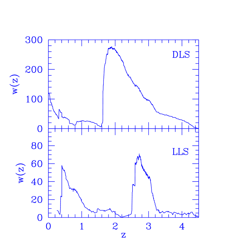
Figure 1: The redshift path density covered by our collection of data.

The redshift path density $w(z)$ (Lanzetta et al., 1991), defined as the number of lines of sight at each redshift searched for LLS with any sensitivity or for DLS with $W\geq 5$, is shown in Figure 1 for all our data. From our data set we extract the LLS sample and the DLS sample. The LLS sample consists of all observations which were sensitive to LLS with $\tau_{LL}\geq 1$. The DLS sample consists of observations sensitive to absorbers with column density log$N_{HI}\geq 20.13$. We wish to examine the number density of absorbers per unit redshift, $dN/dz$ in the LLS and DLS sample. As usual we represent the number density as a power law of the form

$$N(z)=N_{0}(1+z)^{\gamma}$$ (2)

In order to avoid binning the data in redshift intervals, which can generate errors in the estimate of the evolutionary trend, we use the maximum likelihood method described by Storrie-Lombardi et al. (1994) to estimate $N_{0}$ and $\gamma$. For the LLS sample the maximum value of the Likelihood is found for:

$$\gamma=1.66\pm 0.3\qquad N_{0}=0.23$$ (3)

where the errors quoted are the $>68.3\%$ confidence limits. The $>99.7\%$ confidence limits for $\gamma$ are 0.80 and 2.64. These values are similar to the ones obtained by Stengler-Larrea et al. (1995), For the DLS sample we find

$$\gamma=0.86\pm 0.3\qquad N_{0}=0.18$$ (4)

The $>99.7\%$ confidence limits are 0.11 and 1.72. The value of $\gamma$ is consistent but slightly lower than what has been found by Storrie-Lombardi $\&$ Wolfe (2000) for higher column density systems. If we restrict our DLS sample to only those systems with have a measured log$N_{HI}\geq 20.3$ we obtain the same values of $N_{0}$ and $\gamma$ as given by Storrie-Lombardi $\&$ Wolfe (2000). Figure 2 shows the cumulative number of absorbers versus $z$ for both samples. Over plotted is the expected number of LLS and DLS from the Maximum Likelihood estimate. Notice that DLS at $z\geq 1.75$ seem to require a lower value of $\gamma$ than what is given by the Maximum Likelihood estimate over the whole $z$ range. In fact by considering only redshifts $z\geq 1.75$ the match between the data and the best fit cumulative function for DLS improves: in this case $\gamma=-0.07$ with $-1.58$ and 1.36 as $>99.7\%$ confidence limits.

Figure 2: The best fit to the cumulative LLS and DLS number evolution.

For the present paper we shall use data only in the intermediate redshift range $1.75\leq z<3.25$ and for this range the slight difference in evolution implied by eq.  (3) and (4) is unimportant. We use an average $\gamma$ value of 1.0 which is consistent both with the number density evolution of DLS and of LLS. We exclude from the detections absorbers which were declared as “non damped” if they were not detected as LLS or for which no LLS searches have been performed. For “non damped” Ly-$\alpha$ absorbers which were detected as LLS the $N_{HI}$ is set to the value derived from $\tau_{LL}$ when this is available; otherwise we shall use the lower limit to $\tau_{LL}$ for a lower limit to $N_{HI}$ and the column density value derived from $W$ as upper limit.

3 The $N_{HI\perp}-N_{H\perp}$ curve

Our numerical code solves for the ionization, chemical, and hydrostatic equilibrium of a gaseous absorber which receives photons from a background radiation field. It computes the HI column density perpendicular to the plane, $N_{HI\perp}$, in a plane parallel geometry when the total hydrogen column density perpendicular to the plane is $N_{H\perp}$ and the density stratification in the vertical direction $y$ is in the following exponential form:

$$\rho(y)=\rho_{0}{\hbox{exp}}\Bigr{(}-{y^{2}\over 2h^{2}}\Bigl{)}$$ (5)

$\rho_{0}=M_{g}/(\sqrt{2\pi}h)$ is the central gas density for a given total mass surface density per cm^-2 of the gaseous component, $M_{g}$. eq. (5) is the exact solution for the Poisson and first moment equation for an isothermal gaseous disk in equilibrium in a dark matter halo potential in the limit of a negligible self gravity and of negligible changes of the dark matter density with height above the midplane (within the gaseous extent, e.g. Spitzer 1942, Maloney 1993). In this case the scale height can be written as

$${1\over h^{2}}={4\pi G\rho_{dm}\over c_{s}^{2}}={(2\pi G)^{2}M_{dm}^{2}\over c_{s}^{4}}$$ (6)

$c_{s}$ is the sound speed (computed using $T$, the mass averaged temperature of the slab), $\rho_{dm}$ and $M_{dm}$ are respectively the dark matter volume density and the dark matter surface density between +$h$ and -$h$ in the slab. In the absence of dark matter instead eq. (5) is only an approximation to the self gravitating isothermal gas layer solution (e.g. Spitzer 1942)

$$\rho(y)=\rho_{0}{\hbox{sech}}^{2}\Bigr{(}{y\over\sqrt{2}h_{sg}}\Bigl{)}\qquad{1\over h_{sg}^{2}}={2\pi^{2}G^{2}M_{g}^{2}\over c_{s}^{4}}$$ (7)

In this case the gas central density is $\rho_{0}=M_{g}/(2\sqrt{2}h_{sg})$. If we approximate the above exact solution with eq. (5), given the same central volume density $\rho_{0}$ and surface density $M_{g}$, we should use the following expression for the vertical scale height

$${1\over h^{2}}={\pi\over 4h_{sg}^{2}}\simeq{16G^{2}M_{g}^{2}\over c_{s}^{4}}$$ (8)

It will be shown in a subsequent section, that eq. (5), with the scale height $h$ given by eq. (8), is a good approximation to the exact self gravitating gas layer solution for the purposes of this paper. We can therefore write a general expression for $h$ if we use eq. (5) to describe the vertical stratification of the gas when both self gravity and dark matter are taken into account:

$${1\over h^{2}}={16G^{2}M_{g}^{2}\over c_{s}^{4}}(1+\eta^{2})\qquad\qquad{\hbox{with}}\ \eta\equiv{\pi M_{dm}\over 2M_{g}}$$ (9)

The compression factor $\eta$ for the volume density is in general considered as the effect of gravity from matter other than the gas (dark matter, stars or brown dwarfs which coincide with the gas location). We write $\eta$ as

$$\eta\equiv\eta_{0}{c_{s}\over\tilde{c}_{s}}$$ (10)

$\tilde{c}_{s}$ being the value of $c_{s}$ for $T=10^{4}$ K and for a mean gas mass per particle $\mu=1.3$. In this paper we shall consider a set of models, each corresponding to a different $\eta_{0}$ value, and in each model we keep $\eta_{0}$ constant as we very $M_{g}$ while $c_{s}$ is computed from the radiative transfer and energy equation. A constant $\eta_{0}$ value for $\eta_{0}\gg 1$ implies

$$\rho_{dm}\propto M_{g}^{2}$$ (11)

The meaning of the above proportionality are not immediate, but for spherical isothermal dark matter halos eq. (11) implies a constant ratio between the gaseous and dark total surface densities. $\eta$ instead is proportional to the the dark matter surface density between $+h$ and $-h$ and since $h$ scales linearly with $c_{s}$, $\eta$ will also scale with $c_{s}$.

The equilibrium fractional ionizations of H,He,HeII are found step by step through the slab taking into account the diffusion of photons from the recombination of H, He, HeII and the secondary electrons produced by the harder photons. The temperature at each step through the slab is given by balancing photoionization heating with the cooling from hydrogen and helium gas (collisional ionizations, recombinations, lines excitation and free-free processes), from metal lines and from $H_{2}$ cooling. After each iteration the mass averaged temperature $T$ is computed consistently and is used to determine the gas vertical dispersion and stratification. The ionization states of metals (C,O,Fe) are computed step by step consistently with the photoionization rates and charge exchange reactions; very high ionization states (i.e. potential energies $E\gg 54$ eV) are not considered. For metal abundance we use $Z=0.02Z_{\odot}$ throughout this paper but we shall discuss briefly its possible variations. H₂ fractions, although small, are computed via primordial chemical reactions (Corbelli, Galli $\&$ Palla, 1997).

From the ionization-recombination balance we know that for a small neutral fraction the ratio $N_{H\perp}/N_{HI\perp}$ depends on the ratio between the ionization and recombination coefficients and varies inversely with the gas volume density. We define $X$ as

$$X\equiv{\hbox{log}}{N_{H\perp}\over N_{HI\perp}}\qquad{\hbox{for}}\ \ N_{HI}=1.6\times 10^{17}{\hbox{cm}}^{-2}$$ (12)

Notice that $X$ is defined at the line of sight value of $N_{HI}=1.6\times 10^{17}{\hbox{cm}}^{-2}$ and therefore the corresponding $N_{HI\perp}$ value depends on the thickness ratio $h/R$. We derive for $\eta_{0}\geq 1$ the following relation

$$X\simeq 2.94+0.36\ {\hbox{log}}{J_{L}\over\eta_{0}}$$ (13)

where $J_{L}$ is the intensity of the background flux at 912 Å written in units of $10^{-22}$ ergs cm^-2 s^-1 Hz^-1 sr^-1. For our redshift range ($1.75<z<3.25$) we use a constant $J_{L}$ and a flux spectrum computed for $z=2.5$ by Haardt $\&$ Madau (1996, hereafter H-M) for emission by quasars and absorption by intervening clouds. A nearly constant ionization rate between $z=2$ and 4 is also required by comparison of results from hydrodynamical simulations of structure formation with the measured opacity of the Lyman-$\alpha$ forest. The H-M flux intensity at $z\simeq 2.5$, $J_{L}\simeq 5.5$, agrees sufficiently well with other estimates (Rauch et al., 1997; Giallongo et al., 1996) and we shall use $J_{L}=5.5$ throughout. The compression factor $\eta_{0}$ is unknown a priori and will be determined by trial and error. Hence $\eta_{0}$ (or equivalently $X$), and $\alpha$ are parameters to be determined.

Figure 3: The log value of $N_{HI\perp}$ as a function of $N_{H\perp}$ for slabs irradiated by the H-M flux at $z=2.5$ and for log${J_{L}/\eta_{0}}=-1.9,-0.4,0.7$ (from left to right). The dotted vertical lines indicate $N_{H\perp}=9.5\times 10^{16}$ cm^-2 corresponding to $N_{HI}=1.6\times 10^{17}$ cm^-2 for $h/R=0.2$.

In Figure 3 we show three curves for $N_{HI\perp}$ as a function of $N_{H\perp}$ for log$J_{L}/\eta_{0}$ =$-1.9,-0.4,0.7$, which correspond to $X=$ 2.3, 2.8, and 3.2 respectively. All curves in Figure 3 are characterized by 3 regions: a first region at high column density where $N_{H\perp}\simeq N_{HI\perp}$, a second region where for a small change in $N_{H\perp}$ the HI column density changes very rapidly, and a third region, towards the bottom part of the plot, where the log$N_{H\perp}$-log$N_{HI\perp}$ relation is again linear with a slope smaller than unity and which in general depends on the variations of $\eta$ with $N_{H\perp}$. For the models in this paper, we assume that $\eta_{0}$ in eq. (9) does not vary with gas surface density $M_{g}$ (see section 3). The factor ${J_{L}/(1+\eta_{0})}$ is what determines the critical column density where the ${HI\rightarrow HII}$ transition occurs i.e. the column density where the steep slope of the second region starts. The rapidity of the decrease of $N_{HI\perp}$ in the second region depends also on metal abundances. When $Z$ increases above 0.05 $Z_{\odot}$ metal line cooling becomes quite important in that region and the transition gets less sharp as $Z$ increases. The shape of these curves is quite important because it determines the slope of the distribution function around the Lyman-Limit region.

4 From the observed $N_{HI}$ distribution function to the total amount of gas distributed in LLS and DLS.

Several papers on the HI column density distribution of absorbers (Tytler, 1987; Lanzetta et al., 1991; Petitjean et al., 1993) have shown that a power law $N_{HI}^{-1.5}$ fits the data from $10^{13}$ cm^-2 to $10^{21}$ cm^-2 approximately, but not well enough to satisfy statistical tests such as the Kolmogorov-Smirnov test. In this paper we shall use the deviations of $N_{HI}$ distribution from a power law to determine $X$, after assuming that the total gas column density $N_{H}$ has a power law distribution function of the form

$$g(N_{H\perp})=K(1+z)^{\gamma}N_{H\perp}^{-\alpha}$$ (14)

In order to derive the $N_{HI}$ distribution from $g(N_{H\perp})$ we must orient the absorbers randomly in the plane of the sky, assume an axial ratio $h/R$ for the slab, and apply the $N_{H\perp}-N_{HI\perp}$ conversion factor. For our model fitting we shall use $Z=0.02Z_{\odot}$, $X$ independent of redshift and an axial ratio of $h/R=0.2$, since clouds are likely to be neither spherical nor thin disks. Results essentially do not depend on $h/R$ for $h/R\leq 0.5$. We derive $\alpha$ and $X$ by comparing the resulting $f(N_{HI})$ for $\gamma=1.0$ with the data present in our compilation at $N_{HI}\geq 1.6\times 10^{17}$ cm^-2. $K$ is set by the normalization condition for $g$, based on the observed number of absorbers.

We emphasize that it is not possible to present the data relative to the distribution function in a model independent way, due to LLS with undetermined $\tau_{LL}$. A deterioration of the available data might result from the operation of binning in $N_{HI}$ in order to render straightforward the comparison with the model distributions. Instead of binning the data, we match the model distribution to the individual detections. The details of the fitting procedure are given in Paper II; we underline here the main characteristics. The procedure is rather similar to that used by Storrie-Lombardi, Irwin, $\&$ McMahon (1996), but implementing the algorithm in order to take into consideration also the uncertainty in the determination of any single value of $N_{HI}$. Large observational errors are included by leaving undetermined the “real” position of each event. We determine $\alpha$ and $X$ by a Maximum Likelihood analysis to the projected HI column density distribution $f$ fixing the real position of each event to the measured value of $N_{HI}$ when this is available; otherwise we use in the Likelihood the integral of $f$ between the maximum and minimum value of $N_{HI}$. We normalize the theoretical distribution such as to give a number of detections with $N_{HI}\geq 1.6\times 10^{17}$ cm^-2 equal to the observed one. Two maxima for the Likelihood are found:

$$X=2.82\qquad\alpha=2.70\qquad K=1.2\times 10^{34}$$ (15)

$$X=2.74\qquad\alpha=2.57\qquad K=1.8\times 10^{31}$$ (16)

The $>68.3\%$, $>95.5\%$, and $>99\%$ confidence levels in the $X-\alpha$ plane are shown in Figure 4 where the filled dots indicates the location of the maxima as in eq. (15) and (16). The self gravitating gas solution ($\eta=0$, $\alpha=4.63$, $X=3.33$) lies well outside the $>99\%$ confidence level (we would need the 99.999$\%$ confidence level to include it) and therefore it is not consistent with the data. We have also checked that a similar conclusion holds if we use the exact self gravitating gas solution, as given by eq. (7), in deriving the $N_{HI\perp}-N_{H\perp}$ relation. For this case both $X$ and the best fit $\alpha$ value are within $1\%$ of the values obtained using eq. (5) and $\eta=0$ for the vertical gas stratification.

Figure 4: The $>68.3\%$, $>95.5\%$, and $>99\%$ confidence levels in the $X-\alpha$ plane.

In Figure 5 we compare the observed value of the cumulative function with the theoretical ones derived from the integral of the projected HI column density; we show results for the two best fit models (the two maxima in Figure 4) and for two models corresponding to the highest and lowest X values on the $>95.5\%$ confidence level of Figure 4. For points which have no defined $N_{HI}$, i.e. which have large errors, we then compute their best distribution for a given $f$ by spreading the data in the allowed range of $N_{HI}$ according to $f$ weighted with the redshift path. Between all the possible permutations of points with undetermined $N_{HI}$ we then choose those which satisfies best the $U$-test on the deviations between the observed and the expected cumulative functions over the error interval, $R$, and over $N_{HI}$, $C$ (see Paper II for more details and for the use of a numerical simulation to proof the validity of this approach). For $X-\alpha$ inside the $99\%$ confidence level of Figure 4 the K-S tests on $R$ and $C$ are satisfied to the 99.9$\%$ level.

Figure 5: The theoretical cumulative distribution functions (continuous lines) for our two best fit models ($(a)$ $\alpha=2.70$, $X=2.82$ and $(b)$ $\alpha=2.57$, $X=2.74$) and for two points over the $>95.5\%$ confidence level ($(c)$ $\alpha=3.32$, $X=3.07$ and $(d)$ $\alpha=2.27$, $X=2.53$). For comparison the observed HI cumulative functions (dotted lines) are shown.

We have proved that the gas distribution between the LLS and the DLS region follows a single power law with index $\alpha>2$ if the ionization level is such that less than $1\%$ of the total gas is neutral when $N_{HI}=1.6\times 10^{17}$ cm^-2. There is no need of a distribution more complicated than a power law once one takes into account ionization effects. Our results on $\alpha$ and $X$ still hold even if we do not include in the data set the damped lines with $5\leq W\leq 10$ Å or if we exclude a certain percentage of these lines due to possible blending with smaller lines.

4.1 The total gas content of LLS and DLS

We shall discuss here some results relative to the best-fit values of $X$ and $\alpha$ as given in eq. (15) and in eq. (16), and to the two most extreme values of $X$ on the $>95.5\%$ confidence level, namely: $X=3.07$ ($\eta_{0}=2.3$), $\alpha=3.32$ (hereafter $2\sigma$-up); $X=2.53$ ($\eta_{0}=75$), $\alpha=2.27$ (hereafter $2\sigma-$low). The distribution function for the total column density $\tilde{N}_{H\perp}\equiv N_{H\perp}/10^{20}$ cm^-2 can be written as

$$g(\tilde{N}_{H\perp})=\tilde{K}(1+z)\tilde{N}_{H\perp}^{-\alpha}\qquad$$ (17)

In Figure 6, in arbitrary scale, the continuous lines show log $f(N_{HI})$, the HI distribution function, for the best-fit values of $X$ and $\alpha$ as given in eq. (15) and (16), and for the $2\sigma-$low and the $2\sigma$-up models. Our data for $N_{HI}>1.6\times 10^{17}$ cm^-2 is in five large bins just for the purpose of presentation.

Figure 6: HI column density distribution functions between $z=1.75$ and $z=3.25$ for $X=3.07,2.82,2.74,2.53$ and $\alpha=3.32,2.70,2.57,2.27$ respectively (from top to bottom). Bins with open circles have data from our collection while filled triangles are data from the compilation of Petitjean et al. (1993). Scale is arbitrary for each theoretical model but data points have been scaled accordingly.The long dashed line indicates the extrapolation of the distribution function towards the forest region using the same $\eta_{0}$ value as for the LLS and DLS.

$\tilde{N}_{H\perp}\times g(\tilde{N}_{H\perp})$ can be integrated over a range of $\tilde{N}_{H\perp}$, say between $\tilde{N}_{H\perp,i}$ and $\tilde{N}_{H\perp,n}$, to estimate the mass density of hydrogen atoms in gas clouds with an average HI column density along the line of sight between $N_{HI,i}$ and $N_{HI,n}$. The comoving cosmological H+He gas density at $z=2.5$ can be written as:

$${\Omega_{gas}(i)h_{60}}\simeq{2\times 10^{-3}\tilde{K}\over 2-\alpha}{(1+z)\over(1+z)^{\delta}}(\tilde{N}_{H\perp,i}^{-\alpha+2}-\tilde{N}_{H\perp,n}^{-\alpha+2})$$ (18)

$\delta$ depends on the cosmological model and is a function of $z,\Omega_{M},\Omega_{\Lambda}$. For a standard Friedmann Universe in which $q_{0}=0$, $\delta=1$ and we shall use this value for the rest of this section (for $\Omega_{M}=0.3$ and $\Omega_{\Lambda}=0.7$ instead $\delta$ depends on $z$ and is close to zero at $z\sim 2.5$).

In Table 1 we give the values of $\Omega_{gas}(i)h_{60}$, for $i=1,2,3$ which is the total gas density in the Universe at $z\simeq 2.5$ due to absorbing clouds whose HI column density projected along the line of sight is between $N_{HI,i}$ and $10^{22}$ cm^-2. We shall consider $N_{HI,1}=10^{14}$ (see section 4.2), $N_{HI,2}=1.6\times 10^{17}$ and $N_{HI,3}=1.3\times 10^{20}$ cm^-2. For each corresponding value of $N_{H\perp,i}$ we give $X_{i}$, the log ratio of total to neutral gas column density. Results are given both for the best fitting models and for the two most extreme values of $X$ on the $>95.5\%$ confidence level of Figure 4. In the Table we also show the gas scale heights for $N_{HI,2}=1.6\times 10^{17}$ and $N_{HI,3}=1.3\times 10^{20}$ cm^-2, and values of $\Omega_{dark}(i)$.

For $\Omega_{dark}$ in the regions coinciding with the gas the factor $\zeta$ to be substituted into Table 1 is $\zeta\approx 1$, independent of assumptions on cloud size and relative distribution of dark matter and gas. For rotating disks embedded in spherical dark halos one can compute the contribution of the total dark matter surface density to the cosmological matter density. This contribution associated with DLS or LLS systems depends on the rotational velocity $V$ and is given by $\Omega_{dark}$ using $\zeta\approx V/\tilde{c}_{s}$. This factor may be close to one for dwarf clouds, but $\zeta\gg 1$ would hold for giant disk proto-galaxies. For the range of uncertainties in Table 1, the value of $\Omega_{gas}(2)$, the total contribution of LLS plus DLS, varies little but $\eta_{0}$ has a large spread. Consequently, $\Omega_{dark}$ and the gas scale height $h$ also have a large spread. Note that $h(3)$ is particularly small for the $2\sigma$-low limit.

4.2 Conjectures on the Lyman-$\alpha$ forest

The Lyman-$\alpha$ forest clouds may not be directly related to LLS, but we can explore the consequences of two assumption, namely that eq. (17) extends into the Lyman-$\alpha$ forest region with a compression factor $\eta_{0}$ in eq. (9) that has the same constant value as for LLS and DLS. The filled triangles in Figure 6 are the observed data for the Lyman-$\alpha$ forest from Petitjean et al. (1993) and Hu et al. (1995). The dashed curves show the extrapolations of the distribution functions keeping $\alpha$ and $\eta_{0}$ constant. Note that these extrapolations, without any additional parameters, give surprisingly good fits, especially the best fit model given by eq. (15) and the $2\sigma$-up model (the $2\sigma-$low model and the best fit model given by eq. (16) favour a different mechanism of confinement in place for the very low column density clouds, like external pressure, which would steepen the distribution by keeping the fractional ionization of H independent from the cloud column density).

If Lyman-$\alpha$ forest clouds were physically different from LLS and DLS, one might have expected a change in $\alpha$ or $\eta_{0}$ and hence a much worse fit of the dashed curves in Figure 6. The good fit makes it even more likely that $\alpha$ and $\eta_{0}$ are constant from LLS to DLS, which represents a much smaller range in $N_{H}$.

5 Summary and Discussion

The results of the model fit to LLS and DLS presented in this paper underline new aspects in the column density distribution of Lyman-$\alpha$ absorbers:

$\bullet$ The excess of systems in the damped region, suggested by the $N_{HI}$ data, is naturally explained in terms of a sharp transition from a highly ionized to a highly neutral gas distribution and it does not requires any break in the distribution of the total gas column density.

$\bullet$ The total gas column density distributions, $g(N_{H\perp})$, which best fits the data for $1.75\leq z<3.25$ in the LLS and DLS region can be described by a power law of index $-\alpha$ with $2\leq\alpha\leq 3.7$. This has the important consequence that low column density systems contains more mass than high column density systems.

$\bullet$ We have tested that our results, which are relative to the redshift bin $1.75\leq z\leq 3.25$, depend weakly on the data selection and on the number redshift evolution. They also do not show a strong dependence on the assumed thickness to diameter ratio of the slab or from its metallicity if $Z\leq 0.05Z_{\odot}$.

$\bullet$ The gas fractional ionizations increase with decreasing column density and data are best fitted when hydrogen fractional ionizations are of order $\sim 0.002$ at $\tau_{LL}=1$ i.e. $X\sim 2.8$. Gas fractional ionizations for absorbers in a background radiation field depends on the gas volume densities and temperature. The model presented in detail in this paper considers the gas self gravity and a dark matter potential in which the dark matter surface density inside one gas scale height is proportional to the gas surface density (constant $\eta_{0}$). However the range of $\alpha$ and $X$ values compatible with the data are similar if one considers instead a model where $\eta_{0}$ varies with $N_{H}$ (e.g. if $\eta_{0}\times N_{H}$ is kept constant instead). Table 1 summarizes our main results; the values of $\eta_{0}$ for more general models refer to LLS column densities which are no longer opaque to the UV ionizing radiation.

Although our Likelihood analysis allows power law indices $\alpha$ in a rather wide range, 2 to 3.7, other arguments make the upper half of this range more likely: $\alpha\geq 2.7$, $\eta_{0}\leq 13$, $X\geq 2.8$. For larger values of $\eta_{0}$ the gas scale height $h(3)$ for DLS is uncomfortably small and the LLS contribution $\Omega_{dark}(2)$ to cosmological matter density is uncomfortably large (see Table 1, the $\Omega$ values given are for $q_{0}=0$; $\Omega$ values for $\Omega_{M}\sim 0.3$ and $\Omega_{\Lambda}=0.7$ are larger by a factor $\sim 2.5$). For the total dark matter mass, the factor $\zeta$ for $\Omega_{dark}$ is of order $V/10$ km s^-1, which suggests $V<100$ km s^-1 on average for LLS and DLS at redshifts $z\sim 2.5$. This finding is in agreement with the rotational velocities of absorbers halos predicted by Valageas, Schaeffer $\&$ Silk (1999) and with models that propose that a large fraction of Lyman-$\alpha$ absorption systems originate from small low luminosity systems (Abel $\&$ Mo, 1998; Rao $\&$ Turnshek, 2000; Haehnelt, Steinmetz $\&$ Rauch, 2000). However Steidel, Dickinson $\&$ Persson (1994) have shown that small rotational velocities are not required by low redshifts MgII absorption systems with $W>0.3$ Å. These have the same average density per unit path of redshift as LLS and seem to be associated with normal galaxies whose halo extends for $\sim 40$ kpc. This opens the issue about possible evolutionary scenarios for LLS, which can be fully addressed only once we know the redshift evolution of galactic halos and of the galaxy luminosity function. The possible role of faint galaxies as those in pairs close to bright galaxies (Churchill, 2000) should also be taken into account. Futhermore it would be extremely useful to have a larger statistical sample of LLS and DLS at $z<1.75$ and at $z>3.25$ which, together with a better knowledge of the evolution of the background ionizing radiation field, allows a determination of $\alpha$ and $\eta$ at these redshifts (see Paper II for an attempt with the actual data set).

$\bullet$ Although Lyman-$\alpha$ forest clouds, with their much smaller column density, might be physically different and have different values of $\alpha$ and $\eta_{0}$, extrapolations using constant $\alpha$ and $\eta_{0}$ values as for LLS and DLS give surprisingly good fits.

We cannot make definitive statements about the low density Lyman-$\alpha$ forest clouds because of possible dynamic deviations from hydrostatic equilibrium and possible pressure confinement. Nevertheless, the fact that $\alpha$ is appreciably larger than 2 near LLS for $z\sim 2.5$ suggests that forest clouds contained more gas than LLS, which in turn contained more gas than DLS. Several papers have shown that the gas content in DLS at $z\sim 2.5$ is below the mass content in galaxies in the local Universe (Storrie-Lombardi $\&$ Wolfe, 2000), $\Omega_{s+g}h_{60}\simeq 3-7\times 10^{-3}$ and that the stellar mass density in stellar systems at $z\sim 2.5$ is very small (Madau, Pozzetti, Dickinson, 1998). It is therefore likely that gas in forest clouds and LLS at $z\sim 2.5$ has collapsed and contributed to stars in present day galaxies.

We are grateful to P. Madau for providing us numerical results on the background radiation field, to the referee and to Dr. Bothun for very useful comments to the original manuscript, and to D. Chernoff for helping with the Arcetri-Cornell connection. One of us (RB) acknowledges partial support by NSF-PHY94-07194.

Table 1: Ionization and gas content of Lyman-$\alpha$ absorption clouds.

	2$\sigma$-up	best fit 1	best fit 2	2$\sigma$-low
$\alpha$	3.32	2.70	2.57	2.27
$\tilde{K}$	3.81	0.97	0.74	0.42
$\eta_{0}$	2.3	12.5	20.	75.
$X(1)$	5.5	5.2	5.1	4.9
$X(2)\equiv X$	3.1	2.8	2.7	2.5
$X(3)$	0.4	0.2	0.2	0.1
$h(2)$/kpc	2.6	0.8	0.6	0.3
$h(3)$/kpc	1.0	0.3	0.2	0.05
$\Omega_{gas}(1)h_{60}$	0.06	0.01	0.01	0.006
$\Omega_{gas}(2)h_{60}$	0.005	0.004	0.004	0.003
$\Omega_{gas}(3)h_{60}$	0.002	0.002	0.002	0.002
$\Omega_{dark}(1)h_{60}$	0.1$\zeta$	0.2$\zeta$	0.2$\zeta$	0.5$\zeta$
$\Omega_{dark}(2)h_{60}$	0.01$\zeta$	0.05$\zeta$	0.07$\zeta$	0.3$\zeta$

References

- Abel Mo (1998) Abel, T., Mo, H.J. 1998, ApJ, 494, L151
- Bandiera Corbelli (2000) Bandiera, R., Corbelli, E. 2000, ApJ, submitted (Paper II)
- Bergeron Boissé (1991) Bergeron, J., Boissé, P. 1991, A&A, 243, 366
- Churchill (2000) Churchill, C.W. 2000, in Clustering at High Redshift, ASP Conference Series, Vol.200, Ed. by A. Mazure et al., p.271
- Corbelli Salpeter (1993) Corbelli, E., Salpeter, E. E. 1993, ApJ, 419, 104
- Corbelli, Galli Palla (1997) Corbelli, E., Galli, D. Palla, F. 1997, ApJ, 487, L53
- Gardner et al. (1999) Gardner, J.P., Katz, N., Hernquist, L., Weinberg, D.H. ApJ, submitted (astro-ph/9911343)
- Giallongo et al. (1996) Giallongo, E., Cristiani, S., D’Odorico, S., Fontana, A., and Savaglio, S. 1996, ApJ, 466, 46
- Haehnelt, Steinmetz Rauch (2000) Haehnelt, M.G., Steinmetz, M., Rauch, M. 2000, ApJ, 534, 594
- Hu et al. (1995) Hu, E. M., Kim, T-S, Cowie, L. L., Songaila, A., Rauch, M. 1995, AJ, 110, 1526
- Lanzetta et al. (1991) Lanzetta, K. M., Wolfe, A. M., Turnshek, D. A., Lu, L., McMahon, R. G., and Hazard, C. 1991, ApJS, 77, 1
- Lanzetta, Wolfe Turnshek (1995) Lanzetta, K. M., Wolfe, A. M., and Turnshek, D. A. 1995, ApJ, 440, 435
- Madau, Pozzetti, Dickinson (1998) Madau, P., Pozzetti, L., Dickinson, M. 1998, ApJ, 498, 106
- Maloney (1993) Maloney, P. 1993 ApJ, 414, 41
- Petitjean et al. (1993) Petitjean, P., Webb, J. K., Rauch, M., Carswell, R. F., Lanzetta, K. 1993, MNRAS, 262, 499
- Prochaska Wolfe (1998) Prochaska, J.X., Wolfe, A.M. 1998, ApJ, 507, 113
- Rao Turnshek (2000) Rao, S.M., Turnshek, D.A. 2000 , ApJS, in press (astro-ph/9909164)
- Rauch et al. (1997) Rauch, M., et al. 1997, ApJ, 489, 7
- Spitzer (1942) Spitzer, L. 1942, ApJ, 95, 329
- Steidel, Dickinson Persson (1994) Steidel, C.C., Dickinson, M., Persson, S.E. 1994, ApJ, 437, L75
- Stengler-Larrea et al. (1995) Stengler-Larrea, E. A., et al. 1995, ApJ, 444, 64
- Storrie-Lombardi et al. (1994) Storrie-Lombardi, L. J., McMahon, R. G., Irwin, M. J., Hazard, C. 1994, ApJ, 427, L13
- Storrie-Lombardi, Irwin, McMahon (1996) Storrie-Lombardi, L.J., Irwin, M.J., McMahon, R.G. 1996, MNRAS, 282, 1330
- Storrie-Lombardi Wolfe (2000) Storrie-Lombardi, L.J., Wolfe, A.M. 2000, ApJ, in press (astro-ph/0006044)
- Tytler (1987) Tytler, D. 1987, ApJ, 321, 49
- Valageas, Schaeffer Silk (1999) Valageas, P., Schaeffer, R., Silk, J. 1999, A&A, 345, 691
- Wolfe et al. (1995) Wolfe, A. M., Lanzetta, K. M., Foltz, C. B., and Chaffee, F. H. 1995, ApJ, 454, 698