Emissive Mechanism on Spectral Variability of Blazars in High Frequencies

Abstract

The new results of the evolution of the synchrotron peak for Mrk 421 are mostly likely related to the particle acceleration process. In order to account for the above results, we present a model of blazar variability during the flare in which the emission comes from accelerating electrons. A diffusion advection equation of the electron energy distribution is derived to calculate the spectrum and light curve of synchrotron radiation. We present that the observed shifts of the synchrotron peak moving to higher energies during the flare are caused by shock acceleration. The observed relation between changes in the fluxes at specified frequency ranges and shifts of the peak position is fitted to constrain the physical parameters of the dissipation region.

1 Introduction

Among active galactic nuclei, blazars are characterized by a high and variable degree of polarization and a flux variability often occurring on very short time scales. The observed continuum is dominated by nonthermal emission, where the emission deriving from synchrotron and self-Compton is enhanced by relativistic beaming (Blandford & Rees 1978). Some blazars exhibit not only intensity variation extending from radio waves to gamma rays, but also spectral variation as a function of the flux level in many frequency bands.

An interpretation of the spectral variations can be envisaged in an inhomogeneous jet scenario of the kind proposed by Ghisellini et al. (1985) and Celotti et al. (1991). In this model the structure of the jet is considered, the magnetic field and the relativistic electron density are assumed to decrease with distance, and the maximum synchrotron frequency is assumed to decrease with distance, accounting for a variability time shorter at larger synchrotron frequencies. The predicted variability pattern is caused by a disturbance (e.g. shock) traveling down the jet. This perturbation is assumed to produce only a fixed enhancement in magnetic field and particle density and to unchange the shape of the electron distribution. The overall spectrum is the superposition of the located spectra emitted by each slice of the jet. As it has been applied to BL Lac objects, the model does not consider the evolution of the relativistic electron distribution affected by radiation losses, new injection of relativistic electrons and shock waves. However, simultaneous observations of blazars over a wide spectral range suggest that significant radiation losses and injection of relativistic electrons occur in flares. For example, the variability of PKS2155-304 at X-ray, EUV and UV bands is decreased in amplitude and with significant delays approximately satisfying a $\nu^{-\frac{1}{2}}$ relation (Urry et al. 1997). In particular, the radiation loss time for electrons that emit optical and X-ray emission in blazars is probably far less than the light (or the shock) crossing time of the emitting region. Consequently, if the electron distributions responsible for high energy emission are kept by the shock acceleration processes, then radiation losses and the injection of electrons occur in the vicinity of the shock during the flare and must be considered in the theory. Many models to reproduce the spectral variability have been developed ( Mastichiadis & Kirk 1997; Georganopoulous & Marscher 1998; Kirk, Rieger & Mastichiadis 1998; Wang et al. 1999; Ghiaberge & Ghisellini 1999; Li & Kusunose 2000). The observed spectrum and time delays between the light curves at fluxes at different frequencies are believed to be produced by the electron distribution at different stages of evolution after episodic electron injection phases. However these models can not account for a synchrotron peak drifting to higher energies at X-ray wavelengths during the rising phase of the flare in Mrk 421 (Fossati et al. 2000). The above hard lag is most likely related to the particle acceleration process. The role of particle acceleration by shock waves has been considered by Kirk et al. (1998). In this model, electron acceleration and radiation zones are separated. Electrons are continuously accelerated at the shock front, and subsequently drift away from it in the downstream and emit most of the radiation. The emission from the acceleration zone is ignored.

Through shocks can quickly accelerate particles to very high energies, this requires the existence of some scattering agent to force repeated passage of the particles across the shock. The most likely agent for scattering is plasma turbulence or plasma waves. However, the plasma turbulence needed for the scattering can not only accelerate particles stochastically (second order Fermi acceleration), but can cause particle diffusion in the downstream zone quickly. If the dissipation of the bulk energy of blazar jet into particles includes shocks and plasma turbulence, it seems difficult to distinguish acceleration zone and emission region. The emitting particles in downstream could be re-accelerated by shock waves under the scattering of plasma turbulence. Therefore we try to consider the synchrotron emission from a single dissipation region which includes shock and turbulence processes and radiation losses.

In Section II we present a stochastic differential equation to describe a particle acceleration and cooling processes, together with the assumptions made. Then we derive a diffusion-advection equation of particle energy distribution which simulates the temporal evolution of the particle radiation occurring when shock waves and plasma turbulence are produced in a dissipation region of a jet. In section III we apply our model to Mrk 421 to explain the hard lag observed in the X-ray light curves. Finally, we draw our conclusions in section IV.

2 The Model

We focus on the particle acceleration and cooling processes and assume that pitch-angle scattering maintains an almost isotropic particle distribution. We also assume that the shock in a relativistic blazar jet is nonrelativistic, and assume that the light crossing time of the dissipation region is short compared with the intrinsic cooling and acceleration timescales. It is shown that the observed variability is determined by the intrinsic cooling and acceleration processes. We use a homogeneous model in which both the magnetic field and the particle distribution function are assumed homogeneous through the dissipation region, and consider only the synchrotron radiation of the accelerating particles, leaving the more involved computation of inverse Compton emission to future work.

2.1 Evolution of particle energy distribution

Firstly we use a stochastic differential equation (SDE) to describe a particle acceleration and cooling processes, as has been used by some authors (Krülls & Achterberg 1994; Mastichiadis & Kirk 1997). Then we derive a diffusion-advection equation of particle energy distribution (or Fokker-Plank equation). Because the particle distribution is assumed to be isotropic in space and momentum, we consider only the evolution of the particle energy given by

$$\frac{d\varepsilon}{dt}=\stackrel{{\scriptstyle\cdot}}{{\varepsilon}}_{gain}+\stackrel{{\scriptstyle\cdot}}{{\varepsilon}}_{loss}.$$ (1)

The energy losses $\stackrel{{\scriptstyle\cdot}}{{\varepsilon}}_{loss}$ is mainly determined by synchrotron radiation and is a deterministic process in homogeneous model. It has the form

$$\stackrel{{\scriptstyle\cdot}}{{\varepsilon}}_{loss}=-\beta\varepsilon^{2},\qquad\beta=\frac{32\pi e^{4}}{9m_{e}^{4}c^{3}}\left(\frac{B^{2}}{8\pi}\right).$$ (2)

The energy gains $\stackrel{{\scriptstyle\cdot}}{{\varepsilon}}_{gain}$ is due to shock wave and plasma turbulence, and is assumed to have the form

$$\stackrel{{\scriptstyle\cdot}}{{\varepsilon}}_{gain}=a\varepsilon,$$ (3)

where $a$ is a stochastic variable which is determined by mean value $\left\langle a\right\rangle=\alpha$ and a variable $\zeta(t)$ given by the Gaussian noise process, namely it defined by the value $\left\langle\zeta(t)\right\rangle=0$ and the autocorrelation function $\left\langle\zeta(t)\zeta(t^{\prime})\right\rangle=2D\delta(t-t^{\prime})$, where the coefficient $D$ denotes the noise intensity which is assumed to represent the stochastic influence of plasma turbulence. This means that the turbulence will influence the rate of shock acceleration stochastically and cause the particle energy gain to be a random process. To that end one writes Eq(2) as an SDE

$$\frac{d\varepsilon}{dt}=\alpha\varepsilon-\beta\varepsilon^{2}+\varepsilon\zeta(t).$$ (4)

For simplify we have assumed that $\alpha$, $\beta$ and $D$ change slowly compared to particle cooling and acceleration processes, and treat them as constants.

The Fokker-Plank equation corresponding to the system of SDE given in Eq(4) are (Stratonovich 1967)

$$\frac{\partial f(\varepsilon,t)}{\partial t}=-\frac{\partial}{\partial\varepsilon}\left[(\alpha\varepsilon-\beta\varepsilon^{2}+D\varepsilon)f(\varepsilon,t)\right]+D\frac{\partial^{2}}{\partial^{2}\varepsilon}\left[\varepsilon^{2}f(\varepsilon,t)\right],$$ (5)

where $f(\varepsilon,t)$ denotes a conditional probability density $p(\varepsilon,t/\varepsilon_{0},t_{0})$ for any initial energy $\varepsilon_{0}$ at $t_{0}$. If the number $N_{0}$ of particles undergo acceleration, the evolution equation of the particle number density $N(\varepsilon,t)=N_{0}f(\varepsilon,t)$ is similar to Eq(5). In order to include particle escape and injection, we are easy to extend the evolution equation as (Schlickeiser 1984)

$$\frac{\partial N(\varepsilon,t)}{\partial t}=-\frac{\partial}{\partial\varepsilon}\left[(\alpha\varepsilon-\beta\varepsilon^{2})N(\varepsilon,t)\right]+D\frac{\partial^{2}}{\partial^{2}\varepsilon}\left[\varepsilon^{2}N(\varepsilon,t)\right]-\frac{N(\varepsilon,t)}{T_{esc}}+Q(\varepsilon,t).$$ (6)

We consider only the intrinsic cooling and acceleration processes and assume that the timescale of particle is longer than that of the intrinsic physical processes. We ignore the particle escape term in Eq(6). Otherwise we assume that the particles in the dissipation region are accelerated from the initial time $t_{0}$ and no new particle is injected in the following time. The injection term in Eq(6) is also ignored. We scale the energy $\varepsilon$ and the time $t$ as $\varepsilon=\varepsilon_{l}X$ and $t=\alpha^{-1}\tau$, where the critical energy $\varepsilon_{l}=\alpha\beta^{-1}$, and also define $\kappa=D\alpha^{-1}$ which is the ratio of shock acceleration timescale to turbulent acceleration timescale. We can now rewrite the evolution equation of the particle distribution as

$$\frac{\partial N(X,\tau)}{\partial\tau}=-\frac{\partial}{\partial X}\left[X-X^{2}+\delta X\right]N(X,\tau)+\kappa\frac{\partial^{2}}{\partial^{2}X}\left[X^{2}N(X,\tau)\right].$$ (7)

We now turn to finding the solution of Eq(7) describing the evolution of particle distribution. Assume the initial energy distribution of the particles to be $N(X,0)=\delta(X-x_{0})$. We firstly consider the solution of Eq(7) in the case of weak interaction of plasma turbulence $\kappa\ll 1$.

We write $X$ as $X=x(\tau)+\sqrt{\kappa}y$, where $x(\tau)=\left\langle X\right\rangle=\int XN(X,\tau)dX$. Multiplying Eq(7) by $X$ and $X^{2}$ and integrating $X$, we obtain the equation of moments

$$\frac{dx(\tau)}{d\tau}=x(\tau)-x^{2}(\tau),$$ (8)

$$\frac{d\sigma(\tau)}{d\tau}=2\left[1-x(\tau)\right]\sigma(\tau)+2x^{2}(\tau),$$ (9)

where $\sigma(\tau)=\left\langle y^{2}\right\rangle=\int y^{2}N(X,\tau)dX$. Other high order moments can be ignored due to $\kappa\ll 1$. Therefore, the solution of Eq(7) is approximately given by a Gaussian distribution

$$N(X,\tau)=\frac{1}{\sqrt{2\pi\delta\sigma(\tau)}}\exp\left\{-\frac{\left[X-x(\tau)\right]^{2}}{2\delta\sigma(\tau)}\right\},$$ (10)

where $x(\tau)$ and $\sigma(\tau)$ are respectively the solutions of Eq(8) and Eq(9) which are given by

$$x(\tau)=\left[1+(x_{0}^{-1}-1)e^{-\tau}\right]^{-1},$$ (11)

and

$$\sigma(\tau)=C\left[x(\tau)\right]-C(x_{0}).$$ (12)

The function $C(x)$ is defined as

$$C(x)=2(x-x^{2})^{2}\ln\left(\frac{x}{1-x}\right)+x^{4}+4x^{3}(1-x)$$ (13)

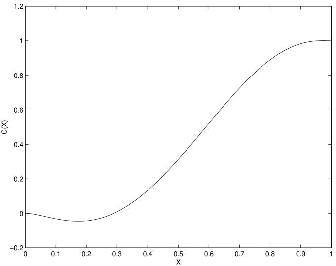
Figure 1: Evolution of the squared variance of particle Guassian energy distribution

shown in Fig.1. Clearly the energy distribution is narrow, centered at a typical energy $\varepsilon_{l}x(\tau)$ and with width $\varepsilon_{l}\sqrt{\kappa\sigma(\tau)}$, quickly evolving with time to $\varepsilon_{l}$ and $\varepsilon_{l}\sqrt{\kappa}$, where $\varepsilon_{l}$ corresponds to the highest energies. It is shown that the particle acceleration is limited by radiation losses

We now consider the solution of Eq(7) for the general value of $\kappa$. It is noted that Eq(7) has a stationary solution given by

$$N_{c}(X)=CX^{\frac{1}{\kappa}-1}\exp\left(-\frac{X}{\kappa}\right),$$ (14)

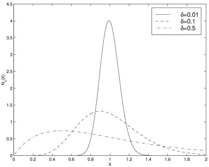
Figure 2: Steady state particle distributions for different turbulent parameters

where $C$ is a normalization constant. The function $N_{c}(X)$ has a peak at $X=1-\kappa$ and a narrow shape with decreasing $\kappa$ which is shown in Figure 2. It indicates that the turbulence leads the spread of the particle energy distribution. The formation of a peak is caused by the interplay of shock wave acceleration, turbulence acceleration and radiation losses

The time-dependent solution can be constructed by eigenfunctions and eigenvalues of Eq(7) (Schenzle & Brand 1979):

$$N(X,\tau)=\sum_{\mu}e^{-\lambda_{\mu}\tau}C_{\lambda_{\mu}}P_{\lambda_{\mu}}(X),$$ (15)

where $P_{\lambda_{\mu}}(X)$ denotes the eigenfuctions of the operator $\widehat{A}(X)$ with eigenvalues $\lambda_{\mu}$, $C_{\lambda_{\mu}}$ are expansion coefficients,

$$\widehat{A}(X)P_{\lambda_{\mu}}(X)\equiv-\frac{\partial}{\partial X}\left[(X-X^{2}+\delta X)P_{\lambda_{\mu}}(X)\right]+\kappa\frac{\partial^{2}}{\partial X^{2}}\left[X^{2}P_{\lambda_{\mu}}(X)\right]=\lambda_{\mu}P_{\lambda_{\mu}}(X),$$ (16)

where $\widehat{A}(X)$ is not an Hermtean operator. The condition of square-integrability and the correlation for the eigenfunctions are

$$\int_{0}^{\infty}N_{s}(X)\left[P_{\lambda_{\mu}}(X)\right]^{2}dX=1,\qquad\int_{0}^{\infty}\overline{P}_{\lambda_{\mu}^{\prime}}(X)P_{\lambda_{\mu}}(X)dX=\delta(\lambda_{\mu}^{\prime}-\lambda_{\mu}),$$ (17)

where the function $\overline{P}_{\lambda_{\mu}^{\prime}}(X)=P_{\lambda_{\mu}}(X)/N_{s}(X)$. From the above condition, the allowed eigenvalues and eigenfunctions are given by

$$\lambda_{n}=n-\kappa n^{2},$$ (18)

$$P_{\lambda_{n}}(X)=N_{s}(X)X^{-n}M(-n,-2n+1+\kappa^{-1},X\kappa^{-1})$$ (19)

for the discrete part of the eigenvalue spectrum, where $n$ is the positive integer subject to the condition $n<\frac{1}{2}\kappa^{-1}$, and a continuous spectrum for $\lambda_{\mu}>\frac{1}{4\kappa}$ with the corresponding eigenfunctions

$$P_{\lambda_{\mu}}(X)=N_{s}(X)X^{i\sigma-\frac{1}{2\kappa}}U(i\sigma-\frac{1}{2\kappa},2i\sigma+1,X\kappa^{-1}),$$ (20)

where $M(a,b,X)$ and $U(a,b,X)$ are Kummer’s function (Abramwitz & Stegun 1970) and $\sigma=\left(\lambda_{\mu}\delta\kappa-\frac{1}{4}\kappa^{-2}\right)^{1/2}$. The expansion coefficients $C_{\lambda_{\mu}}$ are determined from the initial condition

$$C_{\lambda_{\mu}}=\int_{0}^{\infty}N_{s}^{-1}(X)P_{\lambda_{\mu}}(X)N(X,0)dX.$$ (21)

One finally finds

$$N(X,\tau)=\sum_{n}e^{-\lambda_{n}\tau}C_{\lambda_{n}}P_{\lambda_{n}}(X)+\int_{\frac{1}{4\delta^{2}}}^{\infty}e^{-\lambda_{\mu}\tau}C_{\lambda_{\mu}}P_{\lambda_{\mu}}(X)d\lambda_{\mu}.$$ (22)

We now turn to consider the evolution of the particle distribution when the particle acceleration stops and ignore the particle escape. The evolution equation of the particle distribution is given by

$$\frac{\partial N(\varepsilon,t)}{\partial t}=\frac{\partial}{\partial\varepsilon}\left[\beta\varepsilon^{2}N(\varepsilon,t)\right]+N_{s}(\varepsilon)\delta(t-t_{s}),$$ (23)

where $N_{s}(\varepsilon)$ and $t_{s}$ are respectively the particle distribution and the time when the acceleration stops. This case corresponds to the decay phase. The solution of Eq(23) is

$$N(\varepsilon,t)=N_{s}(\varepsilon b^{-1})b^{-2},\qquad b=\left[1-\beta\varepsilon(t-t_{s})\right]\geq 0$$ (24)

which is an extension of the solution given by Kazanas et al. (1998).

3 Application to Mrk 421

A peaked spectrum from observations constrains particle energy distribution to be narrow. It indicates that shock acceleration will dominate particle acceleration processes corresponding to $\kappa\ll 1$. In the following text we focus on the calculation of light curves and spectra in the case of $\kappa\ll 1$. We assume that the initial energy distribution of electrons to be single energy distribution with initial energy $x_{0}\varepsilon_{l}$. The synchrotron emission is calculated from the energy distribution of electrons which is parameterized by the critical energy $\varepsilon_{l}$. We first estimate the parameter $\varepsilon_{l}$ from the timescales of shock acceleration and radiation losses. The timescale $\alpha^{-1}$ of shock acceleration can be estimated in terms of the light crossing timescale $\Delta t$. We assume the timescale $\alpha^{-1}$ to be $\zeta$ times the light crossing timescale, e.g., $\alpha^{-1}=\zeta\Delta t$, one obtain

$$\frac{\varepsilon_{l}}{m_{e}c^{2}}=8.95\times 10^{5}\left(\frac{\zeta\Delta t}{day}\right)^{-1}\left(\frac{B}{0.1G}\right)^{-2}.$$ (25)

The critical frequency is given by

$$\nu_{l}=5.82\left(\frac{\zeta\Delta t}{day}\right)^{-2}\left(\frac{B}{0.1G}\right)^{-3}keV.$$ (26)

We now calculate the synchrotron emissivity as a function of time and frequency $F_{\nu}(\nu,t)$ with

$$F_{\nu}(\nu,t)\propto\int d\varepsilon N(\varepsilon,t)P(\nu,\varepsilon).$$ (27)

$P(\nu,\varepsilon)$ is the single particle synchrotron emissivity which has a approximate function given by Kaplan & Tsytovich (1973):

$$P(\nu,\varepsilon)=a_{s}\sqrt{3}\left(\frac{3}{2}\right)^{1/3}F\left(\frac{\nu}{\nu_{c}}\right),$$ (28)

where $a_{s}=2\pi\sqrt{3}e^{2}c^{-1}\nu_{L}\sin\theta$ is a constant and $\nu_{c}=3\varepsilon^{2}\nu_{L}\sin\theta/(2m_{e}^{2}c^{4})$, with $\nu_{L}=eB/(2\pi m_{e}c)$ the electron Lamor frequency and $\theta$ the angle between the magnetic field direction and the line of sight. The function $F(X)$ is $F(X)=X^{1/3}\exp(-X)$.

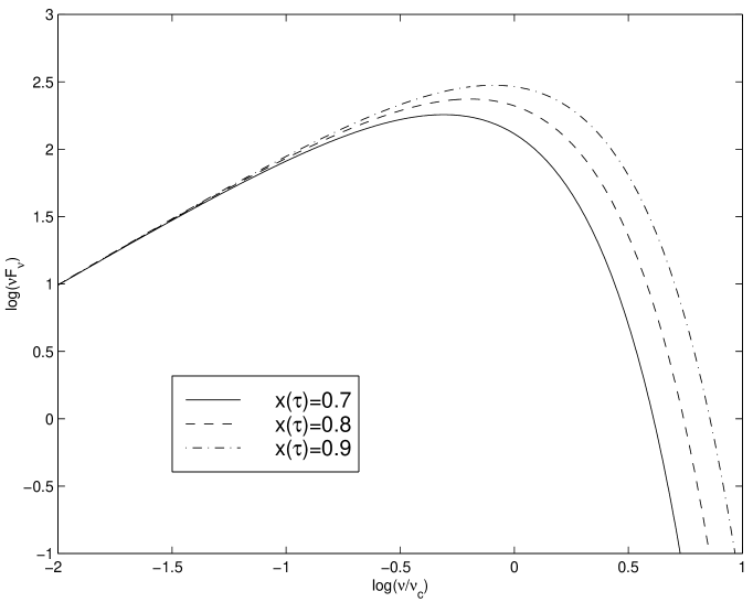
Figure 3: Synchrotron spectral evolution as the central energy of particle distribution is evolving to higher energies

Because the particle distribution is a narrow Guassian distribution, it can be approximated as a Delta function, e.g., $N(\varepsilon,t)=N_{0}\delta(\varepsilon-\varepsilon_{c})$, where $\varepsilon_{c}$ is the central energy of Guassian distribution which is evolving with time ($\varepsilon_{c}=x(\tau)\varepsilon_{l}$). The synchrotron emission is approximated as $F_{\nu}\propto P(\nu,\varepsilon_{c})$. In Figure 3 we plot the synchrotron spectrum $\nu F_{\nu}$ of accelerating electrons at different times. Clearly the synchrotron peak shifts to higher frequencies during the rise. It indicates that the presence of a hard lag is caused by the emission from the electrons which are being accelerated to higher energies by shock wave. The highest energy is determined by the acceleration and cooling rates.

When the shock acceleration stops, the particle distribution will evolve according to Eq(24) due to radiation losses. The corresponding synchrotron emission is given by

$$F_{\nu}\propto\int_{0}^{\varepsilon^{*}}N_{s}(\varepsilon b^{-1})b^{-2}P(\nu,\varepsilon)d\varepsilon,$$ (29)

where $\varepsilon^{*}$ is a cut-off frequency which comes from the limit of $b=\left[1-\beta\varepsilon(t-t_{d})\right]\geq 0$, e.g., $\varepsilon^{*}=\beta^{-1}(t-t_{s})^{-1}$. Using a Delta function to approximate $N_{d}$, e.g., $N_{d}(\varepsilon b^{-1})=N_{0}\delta(\varepsilon b^{-1}-\varepsilon_{c})$, we obtain the synchrotron emission as

$$F_{\nu}\propto\int_{0}^{\varepsilon^{*}}\delta(\varepsilon b^{-1}-\varepsilon_{c})b^{-2}P(\nu,\varepsilon)d\varepsilon=P(\nu,\varepsilon_{t}),$$ (30)

where $\varepsilon_{t}=\varepsilon_{c}[1+\varepsilon_{c}\beta(t-t_{s})]^{-1}$ and $\varepsilon_{c}$ is the central energy of particle Guassian distribution when the shock acceleration stops. Clearly the peak of $\nu F_{\nu}$ decreases to lower frequencies as soon as the shock is over.

The brightness of synchrotron emission at specified frequency ranges $(\nu_{1},\nu_{2})$ for the flare is simply given by

$$L_{f}=\int F_{\nu}d\nu\propto\int P(\nu,\varepsilon_{c})d\nu.$$ (31)

The peak frequency of synchrotron spectrum $\nu F_{\nu}$ locates at $\nu_{p}=\frac{4}{3}\nu_{c}$. The relation of $\nu_{p}$ and $L_{f}$ is

$$L_{f}\propto Q(\nu_{p},\nu_{1,}\nu_{2})=\nu_{p}\int_{3\nu_{1}/4\nu_{p}}^{3\nu_{2}/4\nu_{p}}X^{\frac{1}{3}}e^{-X}dX,$$ (32)

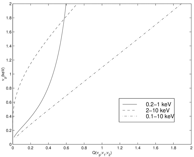
Figure 4: Synchrotron peak energy $\nu_{p}$ versus the fluxes $Q(\nu_{p},\nu_{1},\nu_{2})$ in specified frequency ranges $[\nu_{1},\nu_{2}]$

where the function $Q(\nu_{p},\nu_{1,}\nu_{2})$ is shown in Figure 4. The peak frequencies show an obviously linear relation with the fluxes in 0.1-10keV ranges. This relation reveals the formation of a narrow particle energy distribution by shock wave and the subsequent evolution by radiation losses.

In order to show the above results for application, we thus study the relation between changes in the brightness and shifts of the peak position during the flare based on data of Mrk 421 on 1998 April 21 (Fossati et al. 2000). We introduce a steady spectrum $b(\nu)$ which does not take part in the flare. The observed brightness $L_{obs}$ will include two contributions of the flaring and steady components given by

$$L_{obs}=A\left[Q(\nu_{p},\nu_{1,}\nu_{2})+K(\nu_{1},\nu_{2})\right],$$ (33)

where $K(\nu_{1},\nu_{2})=\int_{\nu_{1}}^{\nu_{2}}b(\nu)d\nu$, and $A=a_{s}\sqrt{3}\left(\frac{3}{2}\right)^{1/3}n_{0}\left(\frac{c\Delta t}{D_{L}}\right)^{2}c\Delta t$ which is given by

$$A=3.0\times 10^{-10}\left(\frac{n_{0}}{10^{7}cm^{-3}}\right)\left(\frac{B}{0.1G}\right)\left(\frac{\Delta t}{hr}\right)^{3}ergs^{-1}cm^{-2}keV^{-1},$$ (34)

where $n_{0}$ is the number density of accelerated particles. $B$ and $R$ are the magnetic field and size of dissipation region respectively. $D_{L}$ is the luminosity distant of source to the observer. We take the Hubble constant to be $50kms^{-1}Mpc^{-1}$and the redshift of Mrk 421 to be $0.031$. The fits of the model are shown in Figure 5. The values of the model parameters are $A=10.0\times 10^{-10}ergs^{-1}cm^{-2}keV^{-1}$and $K=0.08,0.23,0.41keV$ for the 0.2-1, 2-10, 0.1-10keV fluxes. Thus the relation between the spectral evolution and the flux variability during the flare can constrain the physical parameters of dissipation regions. It is important to notice that the inclusion of a steady component is crucial to fit the above relations. The fits of the model indeed achieve the deconvolution of the spectral energy distribution into different contributions. The changes of $K(\nu_{1},\nu_{2})$ with different frequency ranges show that the steady emission concentrates at 2-10keV ranges.

The evolution of synchrotron emission with times is given by Eq(30), where the central energy $\varepsilon_{t}$ evolves during the acceleration and post-acceleration phase as

$$\varepsilon_{t}=\left\{\begin{array}[]{cc}\varepsilon_{l}[1+(x_{0}^{-1}-1)e^{-\tau}]^{-1}&t\leq t_{s}\\ \varepsilon_{t}=\varepsilon_{l}y(\tau_{s})[1+y(\tau_{s})(\tau-\tau_{s})]^{-1}&t>t_{s}\end{array}\right.,$$ (35)

where $y(\tau_{s})=[1+(x_{0}^{-1}-1)e^{-\tau}]^{-1}$, $\tau=\alpha t=\frac{t}{\zeta\Delta t}$ and $\tau_{s}=\frac{t_{s}}{\zeta\Delta t}$. Figure 6 shows the function $F(\nu/\nu_{c})$ of light curves in different frequencies. We find the following interesting results. During the acceleration, the higher energy emissions lag the lower energy ones. The light curve is approximately symmetric in the lower energy bands, and it becomes increasingly asymmetric at higher energies. During the post-acceleration, the light curves are traced in the opposite way. The higher energy emissions first rise and then decays rapidly. The light curve is symmetric in various energies due to the single rise and decay timescale determined by cooling timescale. It should be also noted that the emissions in frequency ranges of $\frac{1}{3}\nu_{l}x_{0}^{2}<\nu<\frac{1}{3}\nu_{l}$ have the light curves of the peak shape due to the maximum value of function $F(\nu/\nu_{c})$ occurring at $\nu=\frac{1}{3}\nu_{l}[1+(x_{0}^{-1}-1)e^{-\tau}]$. The light curves in $\nu\geq\nu_{l}$ bands successively increase to the maximum value of $F(\nu/\nu_{c})$ until the shock wave acceleration stops and then rapidly decay due to particle radiation losses. If the particle escape is not ignored, the variability amplitude in lower energies will decreases in the post-acceleration (Wang et al. 1999). If there is new particle injection during the shock acceleration, higher energy particles will be more than lower energy ones. The larger amplitude variability appears at higher energies.

4 Conclusions

The recent BeppoSAX observations of Mrk 421 (Fossati et al. 2000) provide important information to understand particle acceleration processes. Within a single emission region scenario for blazar jets, we have studied the time dependent behavior of the particle distribution affected by the particle acceleration and radiation losses, and calculated the form of light curves and spectra at different times. We have presented that the observed shifts of the synchrotron peak moving to higher energy during the flare are caused by shock acceleration. The accelerating particles follow a narrow Guassian distribution with a central energy quickly evolving with time to the highest energy when the shock acceleration dominates the turbulent acceleration. The highest energy is limited by radiation losses. Our results are important for the observed fast dissipation region of blazar jets where the light crossing time of the region is shorter than the particle acceleration and cooling time scales. The observed fast variability indicates the particle acceleration and cooling processes.

The observed relation between changes in the fluxes at specified frequency ranges and shifts of the peak position during the flare can estimate the magnetic field and the number density of accelerated particles in the dissipation region.

An energy dependence of the shape of the light curve observed in Mrk 421 during the flare (Fossati et al. 2000) can be connected to the particle acceleration and cooling time scales. During the acceleration, the observed light curves are expected to be symmetric at low energies where the acceleration time is similar to the cooling time and much longer than the light crossing time. The asymmetric light curves (faster rise) occur at higher energies where the acceleration time is shorter than the cooling time and is comparable to the light crossing time. During the post-acceleration, the light curve is symmetric where the rise and decay timescales are equivalent to cooling time scale.

With the steady state solution of the diffusion-advection equation of particle energy distribution, we have demonstrated that the turbulent acceleration leads the particle energy diffusion. The strength of turbulent acceleration determines the width of energy diffusion which modifies the particle distribution with respect to the pure shock acceleration case.

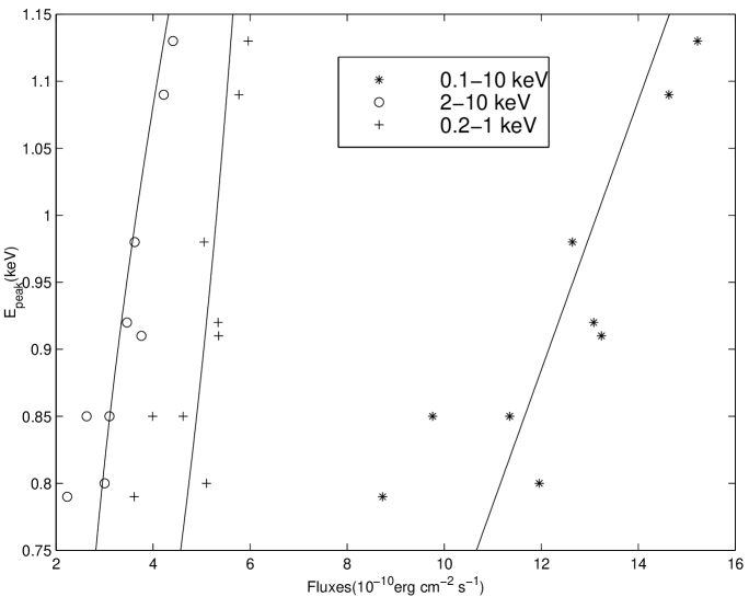
Figure 5: Synchrotron peak energy versus the fluxes in specified frequency ranges for 1998 datasets of Mrk 421. The solid lines represent the best fits of the model

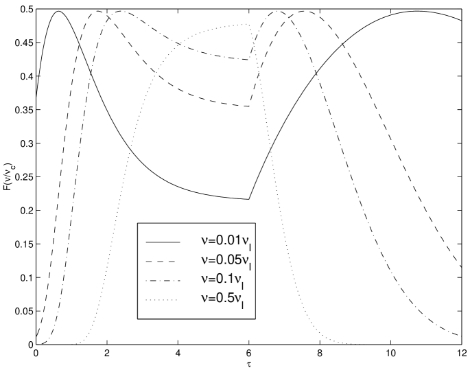
Figure 6: Multiwavelength light curves calculated from $F(\nu/\nu_{c})$ in the case of $X_{0}=0.1$ and $\tau_{s}=6.0$

References

- (1) Abramowitz, M., & Stegun, I. 1970, Handbook of mathematical functions, National Bureau of Stabdards, Washington
- (2) Blandford, R. D., & Rees, M. J. 1978, in Pittsburgh Conference on BL Lac ojects, ed. A. M. Wolfe (Pittsburgh: University of Pittsburgh), P328
- (3) Celotti, A., Maraschi, L., Treves, A. 1991, ApJ, 377, 403
- (4) Chiaberge, M., & Chisellini, G. 1999, MNRAS, 306, 551
- (5) Fossati, G. et al. 2000, ApJ, 541, 166
- (6) Georganopoulos, M., & Marascher, A.P. 1998, ApJ, 506, L11
- (7) Ghisellini, G., Maraschi, L., Treves, A. 1985, A&A, 146, 204
- (8) Kaplan, S.A., & Tsytovich, V.N. 1973, Plasma Astrophysics, Oxford, London
- (9) Kazanas, D., Titarchuk, L.G., Hua, X.M. 1998, ApJ, 493, 708
- (10) Kirk, J.G., Rieger, F.M., Mastichiadis, A. 1998, A&A, 333, 452
- (11) Krülls, W.M., & Achterberg, A. 1994, A&A, 286, 314
- (12) Li, H., & Kusunose, M. 2000, ApJ, 536, 729
- (13) Marcowith, A., & Kirk, J.G. 1999, A&A, 347, 391
- (14) Mastichiadis, A., & Kirk, J.G. 1997, A&A, 320, 19
- (15) Schenzle, A., & Brand, H. 1979, Phys. Lett., A69, 313
- (16) Schlickeiser, R. 1984 A&A, 136, 227
- (17) Stratonovich, R.L. 1967, Topics in the Theory of Random Noise, Vol I, Gordon and Breach, New York
- (18) Urry, C.M. et al. 1997, ApJ, 486, 799
- (19) Wang, J. C., Cen, X. F., Xu, J., Qian, T. L. 1999, ApJ, 519, 556