Galaxy Formation at $z\sim 3$: Constraints from Spatial Clustering

Abstract

We use N-body simulations combined with semi-analytic models to compute the clustering properties of modeled galaxies at $z\sim 3$, and confront these predictions with the clustering properties of the observed population of Lyman-break galaxies (LBGs). Several scenarios for the nature of LBGs are explored, which may be broadly categorized into models in which high-redshift star formation is driven by collisional starbursts and those in which quiescent star formation dominates. For each model, we make predictions for the LBG overdensity distribution, the variance of counts-in-cells, the correlation length, and close pair statistics. Models which assume a one-to-one relationship between massive dark-matter halos and galaxies are disfavored by close pair statistics, as are models in which colliding halos are associated with galaxies in a simplified way. However, when modeling of gas consumption and star formation is included using a semi-analytic treatment, the quiescent and collisional starburst models predict similar clustering properties and none of these models can be ruled out based on the available clustering data. None of the “realistic” models predict a strong dependence of clustering amplitude on the luminosity threshold of the sample, in apparent conflict with some observational results.

Received 2000 November 14; accepted 2000 December 13 The Astrophysical Journal, in press

1 INTRODUCTION

In recent years there has been impressive growth in observations of high-redshift galaxies. The “Lyman-break” technique (Steidel & Hamilton 1992; Madau et al. 1996; Steidel et al. 1996a) makes it possible to select high-redshift candidates based on their photometric colors. Extensive spectroscopic follow-up has confirmed that this technique very reliably selects high redshift ($z\gtrsim 2$) galaxies (Steidel et al. 1996a, b; Lowenthal et al. 1997). The largest sample covers the redshift range $2\lesssim z\lesssim 3.5$, where over 1200 photometric candidates and about 900 spectra have now been obtained, mainly by Steidel and collaborators. Similar techniques can be used to identify galaxies at even higher redshifts, although spectroscopic confirmation is more difficult. About fifty confirmed objects exist at $4.5\lesssim z\lesssim 5.5$ (Steidel et al. 1999) and a handful at $z\gtrsim 5.0$ (e.g., Weymann et al. 1998; Spinrad et al. 1998). Our main focus in this paper will be the $z\sim 3$ LBG sample accumulated by the Steidel group, which is fairly complete to ${\mathcal{R}}=25.5$, allowing robust estimation of the clustering properties at this redshift and magnitude limit.

The correlation length of the $z\sim 3$ sample is similar to that of nearby bright galaxies ($r_{0}\sim 3$–6 ${h^{-1}}$Mpc, comoving; Adelberger et al. 1998; Giavalisco et al. 1998; Giavalisco & Dickinson 2001; hereafter A98, G98 and G00). Within the Cold Dark Matter (CDM) hierarchical structure formation paradigm, these galaxies must therefore be much more clustered than the underlying dark-matter density field (i.e., strongly “biased”). Moreover, because the clustering of matter increases monotonically with time, the bias of the Lyman-break galaxies must be significantly higher than that of typical galaxies at $z=0$. Although the actual level of bias and the details of its redshift dependence depend on the cosmological model and the sample selection, qualitatively this result is quite general and was pointed out by the first observational papers on LBG clustering (A98,G98) as well as numerous subsequent works. This is clearly a key property of high-redshift galaxies and must be explained by any successful theory of galaxy formation.

In the CDM framework, given a power spectrum and a cosmology, the clustering properties of dark-matter halos can be readily estimated, either by analytic methods or using N-body simulations. Numerous groups have shown, using a variety of methods, that the observed clustering and high bias of high-redshift galaxies can plausibly be reproduced in a broad range of CDM cosmologies (Mo & Fukugita 1996; Adelberger et al. 1998; Wechsler et al. 1998; Jing & Suto 1998; Bagla 1998; Baugh et al. 1998; Governato et al. 1998; Coles et al. 1998; Moscardini et al. 1998; Katz et al. 1999; Arnouts et al. 1999; Kauffmann et al. 1999b; Blanton et al. 2000). This implies that the clustering properties of LBGs are not likely to provide very discriminatory constraints on cosmology, especially as long as secure knowledge about their masses is lacking. However, there is still hope that LBG clustering may provide important constraints on galaxy formation.

A remaining central uncertainty is the association of dark-matter halos with observable galaxies. Many previous investigations (Mo & Fukugita 1996; Adelberger et al. 1998; Wechsler et al. 1998; Jing & Suto 1998; Bagla 1998; Coles et al. 1998; Moscardini et al. 1998; Arnouts et al. 1999) have made the simple assumption that every dark-matter halo above a given mass threshold hosts one observable LBG, and that the galaxy luminosity is closely connected with the mass of the host halo. Within the observational uncertainties at the time of publication of these earlier works, the observed number density and correlation length of the $z\sim 3$ sample could be reproduced within this sort of scenario, provided that LBGs were associated with massive halos ($\gtrsim{\rm few}10^{11}{h^{-1}}{\rm M}_{{}_{\mathord{\odot}}}$ for low-$\Omega$ cosmologies). We shall refer to this class of models as “Massive Halo” models for the remainder of this paper.

Kolatt et al. (1999, hereafter K99) investigated a very different model for LBGs, one in which all of the observed high-redshift galaxies are visible because they are temporarily brightened by starbursts triggered by collisions. Colliding halos were identified in a high-resolution N-body simulation, and a simple approach was used to associate these collisions with visible LBGs. Collisions between subhalos can lead to multiple LBGs within the same virialized halo. Although many of the objects in this scenario are far less massive than in the Massive Halo scenario described above, K99 showed that the correlation length of the colliding halos was comparable to that of the observed LBGs, and that the colliding halos were biased with respect to the dark matter. This demonstrated that the mass threshold of the host halos does not uniquely determine the clustering properties of a population of objects. We shall investigate a model similar to the K99 model, which we refer to as the “Colliding Halo” (CH) model.

Though both the Massive Halo and Colliding Halo models were able to simultaneously fit the number density and clustering properties of LBGs, they both rely on an ad hoc connection between dark-matter halos and observable galaxies, and are almost certainly too simple to be correct in detail. More detailed modeling of LBGs, relying on either semi-analytic modeling or hydrodynamic simulations to treat the physics of gas cooling and star formation, has led to a variety of different views regarding the masses and basic nature of the LBG population. Using a semi-analytic model similar to that presented by Cole et al. (1994), Baugh et al. (1998) showed that under their assumptions, LBGs are hosted by massive halos ($\gtrsim 10^{12}{h^{-1}}{\rm M}_{{}_{\mathord{\odot}}}$), and are forming stars mainly quiescently at a moderate rate. The correlation length of LBGs in their model was similar to that obtained in the simpler Massive Halo models and consistent with the observational estimates available at that time (see also Governato et al. 1998). We refer to this picture, in which LBGs are massive, quiescently star-forming objects, as the “massive quiescent” scenario.

Also using semi-analytic models, Somerville, Primack, & Faber (2000b, hereafter SPF) showed that the numbers and properties of high-redshift galaxies in such models are very sensitive to the star formation recipe adopted. They investigated three models, corresponding to three different recipes for star formation, all of which produced good agreement with local observations. In the “Constant Efficiency Quiescent” (CEQ) model, all star formation occurs in a quiescent mode and the star formation efficiency (i.e. the star formation rate per unit mass of cold gas) is constant with redshift. In the “Accelerated Quiescent” (AQ) model, all star formation is quiescent but its efficiency scales inversely with the disk dynamical time, thus increasing rapidly at high redshift. In the third, the “Collisional Starburst” (CSB) model, in addition to quiescent star formation, galaxy-galaxy mergers (both major and minor) are assumed to trigger starbursts — brief episodes in which the rate of star formation is dramatically higher than in the usual quiescent mode. The Collisional Starburst model was favored by SPF as they found that it produced the best overall agreement with the high-redshift data they investigated.

Based on hydrodynamic simulations, Katz et al. (1999) and Weinberg et al. (2000) supported a view intermediate to the massive quiescent scenario of Baugh et al. (1998) and the Collisional Starburst scenario favored by SPF, although closer to the first. Weinberg et al. (2000) found that their simulated LBGs resided within halos with a wide range of masses, but they still reproduced the strong clustering observed. Most of the LBGs in their simulations do not appear to be undergoing starbursts, but the simulations do not have sufficient mass or spatial resolution to properly treat most of the collisions that SPF found to be important.

It is clear that regardless of whether semi-analytic or numerical techniques are used, the results of theoretical predictions about the nature of LBGs depend sensitively on the highly uncertain physics of star formation and feedback. Each of the proposed scenarios has potential problems. The simple Massive Halo models and the more detailed massive quiescent-type models seem to reproduce the observed clustering strength of LBGs, but the “realistic” versions of these models — e.g., the Constant Efficiency Quiescent model of SPF — have difficulty producing enough objects when dust extinction is included, and predict that the number density of bright galaxies should decline rapidly at higher redshift, in apparent conflict with observations (SPF). An alternative recipe for quiescent star formation — the Accelerated Quiescent recipe of SPF — gives acceptable agreement with the number density of LBGs at $z\gtrsim 3$. However, this model has difficulty in producing enough very bright objects, and also consumes so much gas that it violates constraints from observations of Damped Lyman-$\alpha$ systems (SPF) . In addition, because LBGs are found in smaller mass halos, it was not clear whether they would be clustered enough to match the data. The Colliding Halo model of K99 was shown to reproduce the clustering of LBGs on scales of several Mpc, but it may be too clustered on smaller scales, and thus overpredict the number of close pairs (Mo et al. 1999). The clustering properties of the more detailed Collisional Starburst model of SPF have not been checked until the present work, but could suffer the same problem. Also, there is a suggestion that the clustering strength of observed LBGs depends on the luminosity threshold of the sample (Steidel et al. 1998, hereafter S98; G00), with brighter galaxies being more strongly clustered. Because of the expected large dispersion in the relationship between mass and luminosity, starburst models might have difficulty producing a strong trend of this sort.

The goal of this paper is to test a set of models covering the full range of previously proposed scenarios for the nature of LBGs, from the very simple Massive Halo and Colliding Halo models to the more “realistic” models mentioned above, and to determine which of them, if any, can be ruled out by comparing their predicted clustering properties with the available data at $z\sim 3$. The number of observable objects per halo (the occupation function) is calculated using both simple analytic prescriptions and results from the semi-analytic models of SPF. Large-volume dissipationless N-body simulations are used to calculate the expected clustering properties of halos at $z=3$, and the calculated occupation functions are used to convert this into predictions for the clustering properties of observable galaxies (this is similar to the approach used by Kauffmann et al. 1997 and Benson et al. 2000). We mimic the observational selection effects as closely as possible, apply them to model galaxies, and then compare these predictions to the data in the “observational plane”. Throughout the paper, we focus on one cosmology, the currently popular $\Lambda$CDM model, with matter density $\Omega_{m}=0.3$, vacuum energy density $\Omega_{\Lambda}=0.7$, and a Hubble parameter $h=0.7$, where $H_{0}=100h\,\rm{km}\,\rm{s}^{-1}\,\rm{Mpc}^{-1}$.

The outline of the paper is as follows. We begin (§2) with an analytic investigation of clustering for two extreme models for LBGs: Massive Halos and Colliding Halos. In §3, we discuss the data that we will use for comparison. In §4 we discuss the N-body simulations we use to derive halo clustering properties, and the models that are used to populate these halos with galaxies. In §5, we present the statistics used and the results of our comparison. In §6, we compare the Colliding Halo model and the more detailed semi-analytic Collisional Starburst model and determine which elements of the models are responsible for differences in their behavior. We discuss our results and conclude in §7.

2 HALO OCCUPATION AND CLUSTERING

In this section we explore the clustering properties of two toy models representing opposite extremes of the spectrum of proposed scenarios for the nature of LBGs: the Massive Halo model, in which LBGs are associated in a one-to-one fashion with the most massive halos, and the Colliding Halo model, in which LBGs are associated with collisions between halos and/or subhalos. In several previous works (for example A98), the observed clustering of LBGs has been used to obtain estimates of the characteristic masses of their host halos. As shown below, an additional factor in the expected clustering of any population of objects is the average number of objects residing within dark halos of a given mass (the halo occupation function). The unknown occupation function introduces a degeneracy which results in a significant uncertainty in the minimum host halo mass corresponding to a given clustering strength.

For each of our toy models, the halo occupation function $N_{g}(M)$ is approximated as a power-law of the mass for halos larger than some minimum mass $M>M_{\rm min}$: $N_{g}(M)\propto M^{S}$. Here $M_{\rm min}$ corresponds to the minimum mass halo capable of hosting an observable galaxy. The Massive Halo model has the simple form $S=0$ — each halo above some minimum mass is assumed to host exactly one galaxy.

For the Colliding Halo model, a simple approximation for the slope of the occupation function can be obtained using the following argument. Assume that the number of collisions that occur within a halo of mass $M$ over a time interval $\Delta t$ is proportional to the amount of mass that halo has accreted during this time interval divided by the average mass of the accreted objects:

$$N_{\rm coll}\propto\Delta M/<M_{ac}>.$$ (1)

For $\Delta t\ll t$, where $t$ is the age of the universe at the time the halo is observed, we use the single-trajectory formula of Lacey & Cole (1993) in order to estimate the median amount of mass $\Delta M$ accreted by a halo of mass $M$ in a time period $\Delta t$:

$$0.5={\rm erfc}\left[\frac{\delta_{c}(t)-\delta_{c}(t+\Delta t)}{\sqrt{2[\sigma^{2}(M)-\sigma^{2}(M+\Delta M)]}}\right],$$ (2)

where $\delta_{c}(t)=\delta_{c,0}/D(t)$ is the linearly extrapolated critical density, in which $\delta_{c,0}\simeq 1.68$ and $D(t)$ is the linear growth factor. The quantity $\sigma(M)$ is the linear rms fluctuation inside a spherical window of mass $M$, also equal to the square root of the mass power spectrum. If we approximate it as a power law $\sigma(M)\propto M^{-\alpha}$, and assume $\Delta M\ll M$, we find

$$\Delta M\propto M^{1+2\alpha}.$$ (3)

To obtain a rough estimate of the average accreted mass, we approximate the mass spectrum of accreted halos with the power-law form $dN/dM_{ac}\propto M_{ac}^{\alpha-2}$ for $M_{ac}\ll M$ (Lacey & Cole 1993; Press & Schechter 1974). For $M_{\rm min}\ll\Delta M$ this implies

$$<M_{ac}>\simeq\int_{0}^{\Delta M}\frac{dN}{dM_{ac}}M_{ac}dM_{ac}\propto\Delta M^{\alpha}.$$ (4)

Equations 1, 3 and 4 then imply

$$N_{\rm coll}\propto M^{1+\alpha-2\alpha^{2}}.$$ (5)

For our $\Lambda$CDM cosmology at a mass scale of $M\simeq 10^{12}{h^{-1}}{\rm M}_{{}_{\mathord{\odot}}}$, $\alpha\simeq 0.15$, leading to a value of $S\simeq 1.1$. In §4.2.2, we show that this is in reasonable agreement with the results from high-resolution N-body simulations, and with results from semi-analytic Monte Carlo merger-trees. Of course, the approximation should break down for small halo masses $M\simeq M_{\rm min}$.

With simple expressions for the halo occupation function in hand, it is now straightforward to calculate the clustering properties of each model. In the first case, since LBGs are found only in the most massive halos, their clustering will be biased with respect to the underlying dark-matter distribution (see e.g., W98, A98). In the second case, although collisions can be found in smaller-mass halos, they will preferentially be located within large halos, and the distribution of collisions should also be strongly biased.

The bias $b$ is defined here as a relation between the correlation functions of halos and dark matter: $b_{\rm h}^{2}=\xi_{\rm h}/\xi_{\rm DM}$. For halos of mass $M$ at redshift $z$ and on scales large compared to the size of collapsed halos, an approximate expression for the bias is given by Mo & White (1996):

$$b_{h}(M,z)=1+\frac{\nu(M,z)^{2}-1}{\delta_{c}(0)},$$ (6)

where $\nu(M,z)=\delta_{c}(z)/\sigma(M)$.

To do the numerical calculations in this section, we use the expression given by Jing (1999):

$$b_{h}(M,z)=\left(\frac{0.5}{\nu(M,z)^{4}}+1\right)\left(1+\frac{\nu(M,z)^{2}-1}{\delta_{c}(0)}\right),$$ (7)

a modification of Mo & White (1996) which produces better agreement with N-body simulations.

The appropriate bias factor for a population of galaxies within halos more massive than $M_{\rm min}$ is the average of $b_{h}(M,z)$ weighted by the abundance of halos as a function of mass, $dN_{h}/dM$ (e.g., as estimated by the approximation of Press & Schechter 1974; here we use the expression given by Sheth & Tormen 1999 which again is a better fit to simulations), and the average number of LBGs per halo $N_{g}(M)$:

$$b_{g}(z,M>M_{\rm min})=$$ (8)

$$\frac{1}{N_{g}(z)}\int_{M_{\rm min}}^{\infty}\frac{dN_{h}}{dM}(M,z)b_{h}(M,z)N_{g}(M)dM,$$

where $N_{g}(z)=\int_{M_{\rm min}}^{\infty}\frac{dN}{dM}(M,z)N_{g}(M)dM$. For the Massive Halo model, $N_{g}(M)=M^{0}=1$ and the standard expression for the average bias of halos (averaged over a particular mass range) obtains. As above, we use $N_{g}(M)\propto M^{1.1}$ to represent the toy Colliding Halo model.

Bias parameter at z$\sim 3$ (using Equation 7) for halos [$N_{g}(M)=1$] and collisions [$N_{g}(M)\propto M^{1.1}$] as a function of the minimum host halo mass $M_{\rm min}$.

In Figure 2, the galaxy bias is plotted as a function of the minimum host halo mass at $z=3$ for both toy models, assuming our usual $\Lambda$CDM cosmology. Because high-mass halos are weighted more strongly in the Colliding Halo model, galaxies are more biased for fixed $M_{\rm min}$: the observed bias for LBGs in this cosmology ($b\sim 2-3$) corresponds to values of $M_{\rm min}\sim 10^{11}{h^{-1}}{\rm M}_{{}_{\mathord{\odot}}}$ for the Colliding Halo model, versus $M_{\rm min}\sim 10^{12}{h^{-1}}{\rm M}_{{}_{\mathord{\odot}}}$ for the Massive Halo model. This was also shown using N-body simulations by Kolatt et al. (1999), and is discussed further in §5.2.

Note that the above discussion pertains to clustering on scales larger than the sizes of virialized halos. Clustering on smaller scales is extremely sensitive to the slope of the occupation function $N_{g}(M)$, and is discussed further in §5.3. As a final aside, we note that the steep slope of the occupation function for collisions is relevant when estimating the clustering properties of any population believed to be associated with mergers, such as quasars or AGN (e.g., Haiman & Hui 2001; Martini & Weinberg 2001). In the next section we discuss detailed predictions for a number of models for populating halos within an N-body simulation.

3 DATA

Steidel, Adelberger, and their collaborators have compiled a large sample of bright galaxies at high redshifts (S98; A98; Giavalisco et al. 1998; Adelberger et al. 2001). The sample of photometric candidates (based on $U_{n}$, ${\cal G}$, & ${\cal R}$ photometry) now consists of roughly 1300 objects in 15 fields. Spectroscopic redshifts have been obtained for about half this number, and have confirmed that this technique very reliably selects objects in the redshift range $2.2\leq z\leq 3.8$, with a median redshift of $\bar{z}\sim 3$. The photometric sample is estimated to be fairly complete at ${\cal R}\leq 25.5$ (though it remains uncertain whether a significant fraction of the true high-redshift population is missed because the colors lie outside the photometric selection area, for example due to extreme dust reddening; see the discussion in Adelberger & Steidel 2000 and references therein).

In the present analysis, we make use of data from a sample of 500 galaxies with spectroscopic redshifts. Most of these data are published in A98, who found 376 galaxies in this redshift range, in six $9\arcmin\times 9\arcmin$ fields. Also included here is an analysis of an additional two fields of the same size provided to us by K. Adelberger. In order to perform a fair comparison with theoretical predictions, some assumptions must be made about how the observed galaxies are selected. We assume that the true comoving number density of galaxies is constant over the redshift range $2.5\leq z\leq 3.5$, and that the selection function over this redshift range is given by the fit to a histogram of all A98 data. At the peak of the selection function, ($z\sim 3$), we assume that $\sim 70\%$ of all galaxies with ${\cal R}\leq 25.5$ would be identified as photometric candidates (this completeness percentage is still somewhat uncertain, as mentioned above; we choose it so that we match the most recent estimate of the incompleteness-corrected number density given by Adelberger 2000, see below). Spectroscopic redshifts are successfully obtained for $40\%$ of the photometric candidates in this sample; for simplicity (and since the dependence is not yet fully understood) we ignore the probable tendency of the spectroscopic sample to preferentially include brighter galaxies. In addition, the selection function falls off on either side of $z\sim 3$. This implies that the true number density of LBGs in this redshift range with ${\cal R}\leq 25.5$ is about 0.004 h³ Mpc^-3, which is roughly seven times the number density of LBGs with measured redshifts (note that no attempt is made to correct the observations for dust extinction; instead we will apply dust corrections to the theoretical models).

The statistics that we will use to compare with our models are the distribution of overdensities and the variance of counts in cells of roughly 12 ${h^{-1}}$Mpc on a side, the correlation function, and the fraction of galaxies in pairs within $1\arcmin$. The first two quantities are calculated for the spectroscopic sample by A98, and the correlation length is calculated for the photometric sample by G98 and G00. The close pair data were provided to us by K. Adelberger. We also investigate the dependence of the correlation length on the magnitude limit of the sample, which has been discussed in S98 and G00.

4 MODELING

4.1 Halo Clustering: N-Body Simulations

Cosmological N-body simulations are used to obtain the spatial locations and masses of virialized dark-matter halos at $z=3$. The simulations were produced by the GIF collaboration. Only one cosmology is considered here, a flat $\Lambda$CDM model with $\Omega_{m}=0.3$, $h=0.7$, $\sigma_{8}$ = 0.9, and a shape parameter $\Gamma=0.21$. The box is 141 ${h^{-1}}$Mpc on a side, and the simulation includes $256^{3}$ particles of mass $1.4\times 10^{10}{h^{-1}}{\rm M}_{\mathord{\odot}}.$ Virialized halos were identified using a standard friends-of-friends algorithm and only halos with at least 10 particles were used for our analysis (see Kauffmann et al. 1999a for a more detailed description of the halo catalogs).

4.2 Populating Halos with Galaxies

Five different models are considered for populating these halos with observable galaxies. The first two models associate galaxies with either massive halos or halo collisions using very simple, ad hoc prescriptions. For the second set of models, detailed semi-analytic modeling is used in an attempt to calculate the number of observable galaxies per halo from a “forward evolution” approach. The three models in this set correspond to the different recipes for quiescent and bursting star formation considered by SPF. The models are summarized in Table 1, and described in more detail below. Each model is normalized so that the underlying population of galaxies brighter than ${\cal R}=25.5$ has a number density of 0.004 h³ Mpc^-3. The parameters used to obtain this normalization are different for each type of model, and are discussed further below.

Once the halos have been populated with galaxies, we try to mimic the observational selection process by creating an “observed” sample of galaxies according to the assumptions outlined in §3. The simulation box is broken into pixels the size of the data fields, and the galaxies in each pixel are observed according to a selection probability, randomly chosen from one of the data pixels. The resolution of the ground-based images is about $1-2\arcsec$ (K. Adelberger 1999, private communication), so model galaxies within $\sim 1.5\arcsec$ of each other are treated one galaxy.

4.2.1 Massive Halos

In the simplest possible model for LBGs (the Massive Halo model), each halo more massive than a given threshold is assumed to host exactly one LBG. This minimum mass comprises the one adjustable parameter of the model, and is chosen to obtain the observed number density of LBGs. Similar models have been considered previously by many authors (e.g., W98; Adelberger et al. 1998; Jing & Suto 1998; Coles et al. 1998; Moscardini et al. 1998; Bagla 1998; Arnouts et al. 1999).

4.2.2 Colliding Halos

The Colliding Halo model is a simple representation of the idea that galaxies may be made visible by short episodes of star formation triggered by collisions. This model is based on the analysis of a high-resolution N-body simulation which uses the “Adaptive Refinement Tree” (ART) algorithm (Kravtsov et al. 1997) to obtain very high force resolution ($\sim 1h^{-1}$kpc) in a $30h^{-1}$Mpc box. The simulation we use is for the same $\Lambda$CDM cosmology mentioned previously except that here $\sigma_{8}=1.0$ instead of $0.9$. Halo catalogs were created using a variant of a spherical overdensity method (Bullock et al. 2000a) which was explicitly designed to allow the identification of subhalos located within the virial radius of larger halos. Halo and subhalo collisions were then identified using the approach described in Kolatt et al. (1999). The mass per dark-matter particle is $1.25\times 10^{8}{h^{-1}}{\rm M}_{{}_{\mathord{\odot}}}$ and the halo catalogs are complete for halos more massive than $\sim 2\times 10^{10}{h^{-1}}{\rm M}_{{}_{\mathord{\odot}}}$ (Sigad et al. 2001).

The small volume of the ART box does not allow us to robustly calculate some of the clustering statistics directly. The occupation function of collisions is therefore determined by assigning each identified collision to the host halo that it resides in at the end of the timestep. Figure 4.2.2 shows this result for a timestep covering $2.9<z<3.9$, as well as for the same time interval divided into two sub-steps. The average number of collisions per halo as a function of halo mass is very well represented by a power law $N_{\rm coll}\propto M_{\rm host}^{S},$ with a value of $S\simeq 1.13$. This is very close to the power-law slope predicted by the analytic argument in §2. Other timesteps exhibit a similar power law, as does a larger (60 ${h^{-1}}$Mpc), lower resolution box.

This power law is now used to populate the dark-matter halos in the larger, lower resolution GIF simulations with galaxies. We assume that the minimum mass for a halo to host a collision producing a visible LBG is $M_{\rm min}=10^{11}h^{-1}M_{\odot}$. The normalization of the power-law is set by requiring the total number of objects to be the same as the observed density of LBGs. Note that there are sufficient collisions to account for the required normalization in the simulation. For each halo, the actual number of objects is chosen from a Poisson distribution with the mean given by the power-law function: $N=CM^{1.1},M>M_{\rm min}$. The sensitivity of our results to the modeling of scatter is discussed in the following section.

Average number of collisions per halo from the 30 ${h^{-1}}$Mpc ART simulation, for three high-redshift timestep intervals. The error bars shown are 1-$\sigma$ scatter in this value. The best fit slopes for these lines are $1.28\pm 0.07$, $1.03\pm 0.13$, $1.07\pm 0.09$, for the intervals $z=2.9-3.9$, $z=3.3-3.9$, $z=2.9-3.3$, respectively. The heavy line shown is the weighted average for the three timesteps, which yields a slope of 1.13 — similar to the power-law slope value derived from an analytic argument in §2.

4.2.3 Semi-Analytic Models

The Massive Halo model and the Colliding Halo model are not much more than toy models, normalized by adjusting ad hoc parameters. Predicting the number of galaxies within a halo and their luminosities from first principles is a rather daunting proposition. Semi-analytic models attempt to capture the complex interplay of the physics of gravitational collapse and merging, gas dynamics, and star formation and feedback, by using simple recipes to model each of these physical processes. The semi-analytic models used here were developed by Somerville (1997) and are described in SP and SPF. Here we give a brief description of the models, emphasizing the aspects most relevant to the present analysis. The reader is referred to SP, SPF, and references therein for further details.

The formation and merging of dark-matter halos as a function of time is represented by a “merger tree”, which is constructed using the method of Somerville & Kolatt (1999). Halos with velocity dispersions less than $\sim 40\,\rm{km}\,\rm{s}^{-1}$ are assumed to be photo-ionized so that the gas within them cannot cool or form stars. This sets the effective mass resolution of our merger trees. When halos merge, the central galaxy in the largest progenitor halo becomes the new central galaxy and all other galaxies become satellite galaxies orbiting within the halo. Satellite galaxies fall towards the center of the halo due to dynamical friction and eventually merge with the central galaxy. Satellite galaxies may also merge with each other according to the modified mean free path model of Makino & Hut (1997, see SP & SPF for details).

When a halo collapses, the gas within it is assumed to be shock heated to the virial temperature of the halo. This gas is transformed to “cold” gas when the time elapsed since the halo collapsed is equal to the time needed for it to radiate away all of its energy. This “cooling time” depends on the density, temperature, and metallicity of the hot gas.

Quiescent star formation occurs in all disk galaxies that possess cold gas, according to the expression

$$\dot{m}_{*}={m_{\rm cold}\over{\tau_{*}}},$$ (9)

where $m_{\rm cold}$ is the mass in cold gas and $\tau_{*}$ is the “star formation timescale”, which is a parameterization of our ignorance about star formation. SP and SPF considered two cases for quiescent star formation, “constant efficiency”, in which $\tau_{*}$ is constant, and “accelerated”, in which $\tau_{*}\propto t_{\rm dyn}$, where $t_{\rm dyn}$ is the dynamical time of the disk (this is similar to the recipe used by e.g., Kauffmann et al. 1999a). The accelerated recipe is so-named because disk dynamical times are smaller at earlier times, leading to a dramatic increase in the star formation efficiency with redshift. Other authors have considered recipes in which $\tau_{*}$ depends explicitly on circular velocity (Cole et al. 1994; Baugh et al. 1999).

In addition, when galaxies merge, a “burst” mode of star formation may be triggered. The recipe for star formation in bursts adopted by SPF was an attempt to parameterize the results of hydrodynamical simulations of pairs of colliding galaxies (Mihos & Hernquist 1994, 1995, 1996). In a series of papers, Mihos & Hernquist investigated both major (mass ratio 1:1) and minor (mass ratio 1:10) mergers. They found that major mergers typically triggered a burst which consumed 65-80 percent of the available cold gas over several hundred Myr, whereas a minor merger between a satellite and a pure disk galaxy consumed 30-50 percent of the gas over a similar timescale. However, if the larger galaxy possessed a bulge of one-third the disk mass, the burst was suppressed in the minor merger case, and only about 5 percent of the gas was consumed. To attempt to represent this behavior, SPF modeled the burst efficiency (the fraction of cold gas consumed during the burst) as a power-law function of the mass ratio of the merger:

$$e_{\rm burst}=\left(\frac{m_{\rm small}}{m_{\rm big}}\right)^{\alpha}\,,$$ (10)

where the adopted value of $\alpha=0.18$ for the no-bulge case (in which the bulge mass is less than one-third of the disk mass) and $\alpha=1.18$ for the bulge case were chosen to match the two cases simulated by Mihos & Hernquist. We comment later on uncertainties in these parameters, which were all based on simulations of collisions of galaxies which initially resemble low-redshift galaxies. In SPF, the burst timescale was assumed to be equal to the disk dynamical time, which is probably a lower limit on the burst timescale.

Chemical evolution is modeled assuming that each generation of stars produces a fixed yield of metals. These metals are initially deposited in the cold gas, and may be subsequently mixed with the hot halo gas, or ejected from the halo, by supernovae feedback. The luminosity of each galaxy at the desired redshift and in the desired bands is then calculated using stellar population synthesis models. Here we have used the most recent version of the models of Bruzual & Charlot (GISSEL00), and assumed a solar metallicity SED and a Salpeter IMF. We have checked that the results of the GISSEL00 models are consistent with the 1998 versions used in SPF, and that the results presented here are not sensitive to the assumed metallicity of the stellar population.

The semi-analytic models contain a number of free parameters, with the most important being the three that govern the efficiency of quiescent star formation, the efficiency of supernovae feedback, and the yield of metals per solar mass of stars produced. These parameters are set by requiring an average “reference galaxy” (with $V_{c}=220$ km/s) at redshift zero to have the correct luminosity, gas content, and metallicity, as specified by observations of nearby galaxies (see SP for details).

We shall investigate the same three models considered by SPF, which differ only in the treatment of star formation:

1. Constant Efficiency Quiescent (CEQ) : quiescent star formation only (no bursts), and $\tau_{*}\equiv m_{\rm cold}/\dot{m}_{*}=$ constant.

2. Accelerated Quiescent (AQ) : quiescent star formation only (no bursts), and $\tau_{*}\equiv m_{\rm cold}/\dot{m}_{*}\propto t_{\rm dyn}$. For a given halo mass, $t_{\rm dyn}$ is smaller at high redshift because collapsed objects are denser, therefore a given mass of cold gas produces a higher star formation rate in a high-redshift galaxy.

3. Collisional Starburst (CSB) : quiescent star formation is modeled using the “constant efficiency” recipe, and in addition, following mergers, a burst mode of star formation is included using the recipe described above.

These three models produce similar galaxy properties at low redshift, but differ dramatically at high redshift (see SPF).

In this paper, we choose to normalize the number density of objects in each model using an adjustable dust parameter. As in SPF, we assume that the face-on optical depth of the disk depends on the intrinsic rest-UV luminosity of the galaxy via:

$$\tau_{UV}=\tau_{UV,*}\left(\frac{L_{UV,i}}{L_{UV,*}}\right)^{\beta}.$$ (11)

This form was suggested as an empirical description of extinction in low-redshift galaxies by Wang & Heckman (1996). The actual extinction is then calculated by assigning a random inclination to each galaxy and using a “slab” model (see SPF for details). As shown in SPF, this very simple recipe gives remarkably good agreement with the distribution of extinctions for observed LBGs derived by Adelberger & Steidel (2000) based on the slope of the UV continuum. The parameter $L_{UV,*}$ is taken to be the observed value of $L_{*}$ given by Steidel et al. (1999), and we fix $\beta=0.3$, since this value results in the best fit to the luminosity function and is still consistent with the results of Wang & Heckman (1996). The value of $\tau_{UV,*}$ is then adjusted separately for each of the three models in order to match the observed number density of LBGs. Given the assumptions we make for the selection function and number density, the values of $\tau_{UV,*}$ obtained are 0.35, 2.1, and 2.65, for the CEQ, CSB, and AQ model, respectively. A value of $\tau_{UV,*}=1.75$ would correspond to an extinction correction of a factor of five, the average value assumed by Steidel et al. (1999). The more recent results of Adelberger & Steidel (2000) suggest an average extinction of a factor of $\sim 7$, corresponding to $\tau_{UV,*}=2.1$. The extinction required by the CEQ model is therefore a bit low, and for the AQ model a bit high, compared to the best current observational estimates. As these estimates are still fairly uncertain, however, this is not a very serious concern. Note that the number density obtained in the models could be adjusted by tuning other parameters, but at the possible expense of agreement with other data.

4.3 Halo Occupation Functions

The semi-analytic model tells us the probability of observing a galaxy of a given luminosity in a host halo of a given mass. Specifically, we take from each model the probability of observing $N$ objects brighter than ${\cal R}=25.5$ in a halo of mass $M$. In practice, we run a grid of 50 halo masses, and produce 100 Monte Carlo realizations of each mass. Figure 1 shows the average number of objects per halo with ${\cal R}<25.5$ as a function of mass for each model, both before and after dust has been added using the approach described above. The occupation functions for the Massive Halo and Colliding Halo models are also shown.

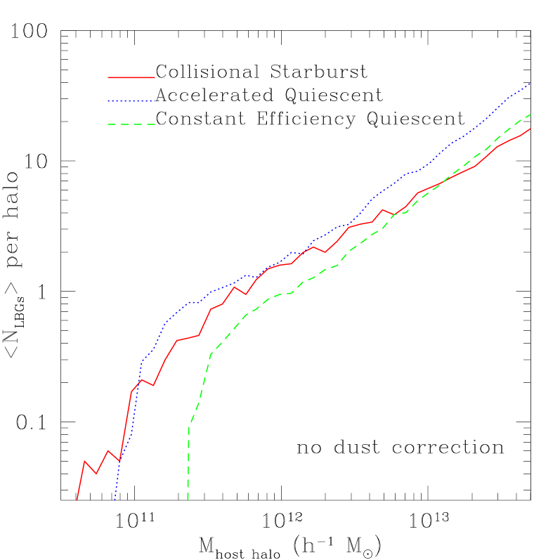
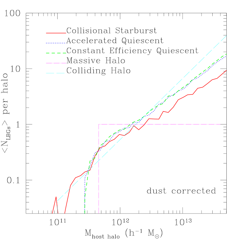
Figure 1: (Left) Average number of galaxies with ${\cal R}\leq 25.5$ per halo for the three semi-analytic models, before (left) and after (right) dust has been added. On the right-hand panel, the occupation functions for the Massive Halo and Colliding Halo models are shown for comparison.

The first thing to note is that all of the models, including the massive quiescent type (represented here by the CEQ model) have much steeper occupation functions than the Massive Halo model. This implies that multiple galaxies in high-mass halos are important even for this class of models. In fact, after the re-normalization using the dust parameter, the quiescent models actually have more multiple galaxies in the massive halos than the Collisional Starburst model. A power-law functional form similar to the one considered in §2 provides a good description of all of the semi-analytic models, with $N_{LBG}\propto M^{0.8}$ on scales larger than a few $\times 10^{11}{h^{-1}}{\rm M}_{{}_{\mathord{\odot}}}$ for the two quiescent models, and a slightly shallower slope of 0.7 for the CSB model.

It is also interesting that the slope of the occupation function for the semi-analytic Collisional Starburst model, $S\simeq 0.7$, is so much shallower than that for the Colliding Halo model, $S\simeq 1.1$. This must be either because the approximations used to model the collisions of halos in the semi-analytic models are inaccurate, or because of the more detailed modeling of the luminosity associated with each collision in the semi-analytics. This is investigated in detail in §6; it is primarily due to the luminosity assignment, in the sense that mergers are less likely to produce visible LBGs in massive halos.

Figure 1 shows only the mean number of galaxies in halos as a function of their mass; an important additional piece of information is the scatter in this quantity. Benson et al. (2000) have shown that the scatter is important in determining the small-scale clustering properties. For the Massive Halo model, we simply assume that each halo has zero or one galaxy, with no scatter. For the Colliding Halo model, the number of galaxies is drawn from a Poisson distribution. For the semi-analytic models, the scatter is provided from 100 Monte Carlo realizations of each halo.

Once the number of galaxies is chosen, they must be assigned positions within the halo; the first galaxy is placed at the center of the halo, and the additional galaxies are placed randomly in radius within $R_{\rm vir}$, which corresponds to an isothermal density distribution, and is also in rough agreement with the results of the ART simulation. This placement is somewhat uncertain; however, none of the statistics considered here are very sensitive to the internal structure of the halo.

5 COMPARING MODELS WITH DATA: RESULTS

5.1 Weighted Overdensity

A standard statistic for measuring the clustering of a population is the overdensity in some region; in Wechsler et al. (1998), we looked at the distribution of LBG overdensities in cells that were $\Delta z=0.04$ in redshift and $9\arcmin\times 9\arcmin$ on the sky, and compared to the data from just one field — 13 cells (from A98). Explicitly, the raw counts $N_{i}$ were de-selected into

$${\cal N}_{i}=N_{i}/S_{i},$$ (12)

where $S_{i}$ is the selection function in pixel $i$. From then on, using the statistic

$$d_{i}\equiv\delta{\cal N}_{i}/\bar{\cal N}=\delta N_{i}/\bar{N}_{i},$$ (13)

where $\delta N=N/\bar{N}-1$, all the pixels were treated equally. By doing that, we ignored the fact that the Poisson errors, which depend on $S_{i}$, affect the probability distribution function (PDF) of $d_{i}$. In particular, it is “easier” to obtain more extreme density contrasts where the error in that quantity is larger, i.e., where $S_{i}$ is smaller. This rather gross approximation was worst when assigning a single value of $p$ (the probability of getting a spike of a particular size in one pixel) to all the pixels and then translating it to $P_{1}$ (the probability that a spike of this size is chosen in all pixels); in fact, the actual probability $p_{i}$ should vary with $S_{i}$, and $P_{1}$ should be computed accordingly. Our excuse, which was fine as a first approximation, was that only pixels with $S_{i}\geq 0.4S_{max}$ were included, and thus the error was kept relatively small.

With the extended data from several fields we can now be more accurate, and can also include pixels with smaller $S_{i}$. The first goal is to find a statistic that would indeed put all the pixels on the same footing. Such a statistic is the error weighted galaxy overdensity:

$$D_{i}\equiv{\delta{\cal N}_{i}/\bar{\cal N}\over\sigma_{i}},$$ (14)

where $\sigma_{i}$ is the Poisson error in the quantity of interest, $d_{i}$, which measures fluctuations in the real universe.

Since the Poisson error in $N_{i}$ is $\bar{N}_{i}^{1/2}$ (ignoring additional factors proportional to $J_{3}$ in case of correlations), it follows from equations 12 and 13 that $\sigma_{i}=\bar{N}_{i}^{-1/2}$, and thus

$$D_{i}={\delta N_{i}\over\bar{N}_{i}^{1/2}}.$$ (15)

The square-root $\bar{N}_{i}^{1/2}$ in the denominator replaces the $\bar{N}_{i}$ in the denominator of the old statistic. With the new statistic, a spike of a given positive true relative over-density $d_{i}$ that occurs where $S_{i}$ is lower than $S_{max}$ is now associated with a smaller $D_{i}$ compared to a spike of a similar $d_{i}$ at $S_{max}$. This takes into account the fact that larger density contrasts are more likely to occur where $S_{i}$ is small.

The statistic $D_{i}$ describes the count fluctuations in terms of the rms Poisson fluctuations in each pixel. If there are enough LBGs expected on the average, the distribution of $D_{i}$ approaches that of a Gaussian with width unity. Then it is perfectly consistent to consider all the pixels together on the same footing, and one could use Gaussian statistics to evaluate probabilities. Since we are not really in the Gaussian limit, the PDFs in the different pixels are not exactly the same, although they are far closer to each other than before. To deal with this imperfection, the comparison of the data and models is pursued in the “observational plane”: we apply the observed selection function to the simulated counts and then compute the statistic $D_{i}$ and construct its PDF by the distribution of its value over the pixels. This PDF is then compared to the PDF constructed directly from the data.

Probability distribution of the error-weighted galaxy overdensity for the five models, compared with eight fields of data (shaded), from A98 and Adelberger et al. (2001).

For each model, the differential distribution of this statistic is compared with that of the data (Figure 5.1) using the Kolmogorov-Smirnov (KS) test, which gives the probabilities that the data and the model came from the same underlying distribution. The results are shown in Table 2, and show that none of the models can be ruled out. The KS statistic, however, can systematically underestimate the significance of differences between the observations and the models, especially if the differences are near the ends of the distribution (Press et al. 1992). Kuiper’s variant of this test (Kuiper 1962; Press et al. 1992) uses the sum of the maximum positive difference and the absolute value of the maximum negative difference, instead of the the maximum of the absolute value of the difference between observed and expected cumulative counts used by the standard KS test, and does not suffer from these problems. The values for this test are also listed in Table 2. In this analysis, there are 192 data pixels and 720 simulation pixels, each $9\arcmin\times 9\arcmin$ on the sky and $\Delta z=0.04$ in redshift. The assignment of galaxies to halos and “observation” of LBGs is done 10 times for each model; the numbers quoted in the table are the mean and error on the mean of these runs. Unfortunately, none of the models can be ruled out even using this modified statistic; even the two extreme halo models cannot be distinguished from the data at present. However, it should be noted that we are comparing to an observational sample with only 500 galaxies. With two to three times more data (much of which already exists but is unpublished), these statistics will become discriminatory.

Table 1: Models of Lyman-Break Galaxies

Model	halo occupation: $N(M)\propto M^{S}$	normalization	star formation/luminosity assignment
Massive Halo (MH)	$S=0$, no scatter	Mass cut	$L\propto M$, $M>4.5\times 10^{11}$
Colliding Halo (CH)	$S=1.1$, Poisson scatter	C, $N(M)=CM^{S}$	$L\propto(M_{1}+M_{2}),M_{\rm host}>10^{11}$
Collisional	semi-analytic, $S\sim 0.7$	dust, $\tau_{UV}=2.1$	quiescent, $\tau_{*}=$ constant
Starburst (CSB)			+ starbursts
Constant Efficiency	semi-analytic, $S\sim 0.8$	dust, $\tau_{UV}=0.35$	quiescent, $\tau_{*}$ = constant
Quiescent (CEQ)
Accelerated	semi-analytic, $S\sim 0.8$	dust, $\tau_{UV}=2.7$	quiescent, $\tau_{*}\propto t_{\rm dyn}$
Quiescent (AQ)

Table 2: Kolmogorov-Smirnov and Kuiper Probabilities and Correlation Function Parameters

	PDF probabilities		Counts-in-Cells		3-space Correlation Function
Model	K-S	Kuiper	$\sigma^{2}_{gal}$	$r_{0}$ [${h^{-1}}$Mpc]	$r_{0}$ [${h^{-1}}$Mpc]	$r_{0}$ [${h^{-1}}$Mpc]	$\gamma$
	probability	probability		$\gamma$=1.6	$\gamma$=1.6	$\gamma$ free
MH	$0.71\pm 0.06$	$0.66\pm 0.08$	$0.69\pm 0.10$	$4.1\pm 0.4$	$4.62\pm 0.18$	$4.65\pm 0.20$	$1.51\pm 0.09$
CH	$0.92\pm 0.03$	$0.82\pm 0.03$	$1.19\pm 0.18$	$5.9\pm 0.5$	$5.59\pm 0.27$	$5.60\pm 0.30$	$1.62\pm 0.10$
CSB	$0.73\pm 0.05$	$0.78\pm 0.06$	$0.69\pm 0.11$	$4.2\pm 0.5$	$4.62\pm 0.24$	$4.64\pm 0.24$	$1.52\pm 0.11$
CEQ	$0.81\pm 0.06$	$0.76\pm 0.04$	$0.90\pm 0.13$	$4.9\pm 0.4$	$5.26\pm 0.21$	$5.29\pm 0.24$	$1.58\pm 0.09$
AQ	$0.80\pm 0.04$	$0.71\pm 0.06$	$0.88\pm 0.12$	$4.9\pm 0.4$	$5.16\pm 0.28$	$5.20\pm 0.29$	$1.57\pm 0.10$

Table 3: Observational Correlation Function Parameters

Sample	Method	magnitude limit	$r_{0}$ [${h^{-1}}$Mpc]	$\gamma$	reference
SPEC	CIC	${\cal R}=25.5$	$6\pm 1$	[1.8]	Adelberger et al. 1998
SPEC	CIC	${\cal R}=25.5$	$4.4\pm 0.9$	$[1.6]$	Adelberger 2000
SPEC	$w(\theta)$	${\cal R}=25.5$	$3.8\pm 0.3$	$1.61\pm 0.15$	Adelberger 2000
SPEC	CIC	${\cal R}=25.0$	$5.0\pm 0.7$	$[2.0]$	Giavalisco et al. 2001
PHOT	$w(\theta)$	${\cal R}=25.5$	$3.2\pm 0.7$	$2.0\pm 0.2$	Giavalisco et al. 2001
HDF	$w(\theta)$	$V_{606}=27$	$1.2^{+0.9}_{-0.8}$	$2.2^{+0.6}_{-0.3}$	Giavalisco et al. 2001
HDF photo-z	$w(\theta)$	$I_{814}=28.5$	$2.78\pm 0.68$	[1.8]	Arnouts et al. 1999

5.2 Two-Point Correlation Function

We use the standard notation for that ubiquitous measure of clustering, the correlation function, $\xi(r)=(r/r_{0})^{-\gamma}$. The observed correlation length $r_{0}$ of a sample with redshift information may be estimated either from a counts-in-cells analysis (assuming a value for $\gamma$), or by inverting the angular correlation function (e.g., Peebles 1980). For our usual $\Lambda$CDM cosmology, the initial estimate using the first method yielded a value of $r_{0}\sim 6$ ${h^{-1}}$Mpc (A98), whereas the second method yielded lower values of $\sim 3-4$ ${h^{-1}}$Mpc (Adelberger 2000). However, more recent observational estimates give lower values of roughly $r_{0}\sim 4.4$ ${h^{-1}}$Mpc and $r_{0}\sim 3.1$ ${h^{-1}}$Mpc (K. Adelberger 2000, private communication) for the counts-in-cells and $w(\theta)$ methods respectively.

Using the angular correlation inversion method on a fainter sample ($V_{606}<27$) of LBGs in the HDF, G00 obtained even smaller correlation lengths, $1.4-1.7$ ${h^{-1}}$Mpc. However, the analysis of Arnouts et al. (1999), based on galaxies in the HDF with photometric redshifts in the range $2.5<z<3.5$ and $I_{814}<28.5$, yields $r_{0}\sim 3$ ${h^{-1}}$Mpc, consistent with the brighter ground-based samples (see also Magliocchetti & Maddox 1999). The correlation function parameters obtained from the observations, calculated for our $\Lambda$CDM cosmology, are summarized in Table 3. We return to the possibility of luminosity segregation in §5.4, and for the moment concentrate on the brighter (${\cal R}_{AB}<25.5$) ground-based samples with spectroscopic redshifts.

Since different methods of estimating the correlation length may give different values, and since the selection function of the observational sample may also affect the result, we calculate the correlation length from our simulations in two ways. First, we simply calculate the real-space correlation function in three dimensions, using all of the galaxies brighter than ${\cal R}_{AB}<25.5$ in each model, randomly sampled to match the observed number density (different selection probabilities for different regions are not used in selecting galaxies for this method, since this would bias the results). The real-space correlation function for all five of our models is shown in Figure 5.2. The errors quoted represent the $1\sigma$ scatter in the results of 100 resamplings and reassignments of galaxies to halos. The best fit values for the correlation length are listed in Table 2 for $\gamma$ fixed to 1.6 and for $\gamma$ left as a free parameter. In each case we only fit the data on scales between 1–8 ${h^{-1}}$Mpc, where the errors and the deviation from a power law are small; we concentrate on scales smaller than this in the next section.

The counts-in-cells method estimates the correlation length by measuring the variance of galaxy counts in spatial bins of a given size:

$$\sigma^{2}_{\rm gal}=[\langle(N-\mu)^{2}\rangle-\mu]/\mu^{2},$$ (16)

where $\mu$ is the expected number of galaxies in a cell, equal to the total number density of observed galaxies times the probability of observing a galaxy in that cell. Subtracting the $\mu$ term removes shot noise, since the average number of galaxies per cell is small. We follow the method of Adelberger et al. (1998) as closely as possible to estimate this statistic for our sample: we break the box into cubical cells, which for this cosmology have a length of 11.4 ${h^{-1}}$Mpc, select the galaxies in each cell with a fraction drawn from one of the data cells, calculate the estimator $[(N-\mu)^{2}-\mu]/\mu^{2}$ for each cell, and then combine the estimates from each cell with inverse-variance weighting for a final estimate of $\sigma^{2}_{\rm gal}$. If the correlation function is a pure power law, for spherical cells the correlation length is given by: $r_{0}=R_{\rm cell}[\sigma^{2}_{\rm gal}(3-\gamma)(4-\gamma)(6-\gamma)2^{\gamma}/72]^{1/\gamma}$ (Peebles 1980). The values of $\sigma^{2}_{\rm gal}$, and the corresponding values of $r_{0}$ (taking $R_{\rm cell}$ to be the radius of a sphere with volume equal to that of our cubical cells) are given in Table 2. These should be compared to the current value obtained from the observational sample: $\sigma^{2}_{\rm gal}=0.75\pm 0.25$ (Adelberger 2000; note that the value from the earlier published work of A98 was $\sigma^{2}_{\rm gal}=1.3\pm 0.4$). If, instead of the selection procedure described above, each cell is just randomly selected with the same probability, the results are essentially unchanged. Note that the errors listed in the table are the variance over 100 re-samplings of our entire box; the variance over regions the size of the full data sample used here (approximately three times smaller) is quite close to the error quoted on the data — roughly  0.2 in $\sigma^{2}_{\rm gal}$. Unfortunately, it is not straightforward to calculate the angular correlation function from the simulation in a way that would be meaningful for comparison to the data, since our box is not large enough to have the same angular projection effects as the data.

Correlation function for all five models. Also plotted are the most recent best-fit parameters, with shaded error regions, from the observations, for the counts-in-cells method (horizontal shading), and the inversion of the angular correlation function (vertical shading).

The two methods presented here give fairly similar results, although for most of the models the counts-in-cells method gives a slightly lower value than that estimated directly from the three-space correlation function. The biggest discrepancies are for the Massive Halo and Colliding Halo model: in the former the counts-in-cells method gives a significantly lower value, in the latter it gives a higher value. The reason for this is easy to understand — the counts-in-cells method is sensitive to clustering on all scales smaller than the cell size, and assumes that the correlation function is a power law over this full range. As can be seen from Figure 5.2, in the Massive Halo model, the correlation function is shallower than a power law on small scales, while in the Colliding Halo model, it is steeper.

The various models actually have quite similar correlation lengths, and all of the models, with the possible exception of the Colliding Halo model, are within reasonable agreement with the counts-in-cells estimate from the data. The latest estimate, for the same sample, from the inversion of the angular correlation function, however, is quite a bit lower (see Table 3) — if this value turns out to be correct, all of the models presented here may be in trouble. There may be more hope of distinguishing the models using their clustering on small scales; we focus on this in the following section.

5.3 Close Pairs

From examining Figure 1, it is clear that a major difference between our five models is the number of multiple objects within one halo. Although this cannot be directly observed, one can determine the number of pairs of objects at small angular separations in the models, and compare directly to observations. “Pairs”, in the sense used here, are objects within a given angular separation which are also within a redshift interval of $\Delta z=0.04$. This definition is used for both the data and the models.

Figure 5.3 shows, for angular separations between 0 and $60\arcsec$, the number of pairs divided by the total number of galaxies for all five models, compared with the data. One might be concerned that the true number of close pairs would be underestimated if there was a bias against obtaining spectra for close pairs, due for example to the physical limitations of slit placement on the masks. However, each field is typically observed with several independent masks so that this effect is not very large. For example, for a sub-sample of candidates that includes 109 pairs of objects within $10\arcsec$ of each other, spectroscopy is obtained for half of the objects, and is obtained for both objects in 21 of the pairs (K. Adelberger 1999, private communication), instead of the number that would be expected with no bias — $109\times 0.5^{2}=27.25\pm 5.2$. This suggests that the systematic error from selection against close pairs is less than about 25%.

In Figure 5.3, the only significant differences between the models are in the first bin, which at $z\sim 3$ corresponds to a comoving distance of $\sim 300$ ${h^{-1}}$kpc (a physical size of $\sim 80$${h^{-1}}$kpc, which is roughly the virial radius of a $10^{12}{\rm M}_{{}_{\mathord{\odot}}}$ halo) for this $\Lambda$CDM cosmology, and includes most galaxies that are in the same halo. However, models which are dominated by galaxies in more massive halos will depend more sensitively on the distribution within the halo. Still, the determining factor in the number of pairs in this bin is mainly the number of multiple galaxies in massive halos, or, since all the models have been normalized to have the same total number density, the slope and cutoff of the halo occupation function, $N_{LBG}(M)$, that was discussed in §4.3. The Massive Halo model, in which all the pairs reside in different halos, underpredicts the number density of close pairs by more than $1.5\sigma$. Conversely, the Colliding Halo model overpredicts the number of pairs within $15\arcsec$ by almost $4\sigma$. However, we find that all three “realistic” semi-analytic models, including the Collisional Starburst model, match the data at least reasonably well, especially given that the number of spectroscopic pairs may be underestimated somewhat. In fact, the quiescent models actually predict more close pairs than the Collisional Starburst model. This is counter to naïve expectations, but follows from what we found in §4.2.3 — that each massive halo actually has more LBGs in the quiescent models.

Number of pairs divided by total number of galaxies for the models (symbols; the plotted horizontal locations are shifted slightly for clarity), compared with the data ($1\sigma$ error on the mean of eight fields is plotted with shaded boxes). Errors plotted for the models are the $1\sigma$ scatter of 50 re-samplings each of three different regions of the box, each the same volume as the total data sample. The typical error due to cosmic scatter is shown in the lower right corner of the plot.

Although the models primarily differ from each other on spatial scales smaller than the size of the most massive halos (which are mostly within the first and second bin of Figure 5.3), all of the models seem to underpredict the number of pairs at intermediate separations, specifically from 30-45″— though the number of observed objects suffers from small number statistics, and this seems a likely cause of the discrepancy. At these separations, the close pair statistics are mostly determined by the clustering of the dark halos. Adjusting the cosmology or other details of the models may improve the predictions, or perhaps the selection is not completely understood. It should also be noted that we have ignored any correlation in the galaxy properties on scales larger than the halos themselves — i.e., the dependence of galaxy formation efficiency on the large-scale environment (obviously, correlation between the dark halos themselves is built into the halo catalog). One might imagine, for example, that the details of the galaxy luminosities could be dependent on the merger history of the halos, which may depend on the larger scale environment. This is explored further in future work (Wechsler 2001).

As noted earlier, and as emphasized by Benson et al. (2000), the clustering strength on small scales depends on the scatter in the halo occupation function. In the models presented here, we assumed no scatter for the Massive Halo model, Poisson scatter for the Colliding Halo model, and the actual scatter given by the full semi-analytic treatment for the other three models. In all cases, we find that including scatter increases the small-scale correlations. The scatter from the semi-analytic models results in slightly lower correlations than Poisson. In the case of the Colliding Halo model, using the mean decreases the pair fraction in the first bin by about 0.03 — far from sufficient to reconcile it with the data. An alternative to looking directly at close pairs would be to compare the scale dependence of the bias. It is clear from Figure  5.2 that the Colliding Halo model is significantly more biased on small scales than on large scales, and the reverse is true for the Massive Halo model — so this might be another possible discriminant if it was well measured in the data.

5.4 Dependence of Clustering on Luminosity

There have been suggestions (S98, G00) that the clustering strength of LBGs depends on the magnitude limit of the sample, or similarly on the number density of the population. These authors compared the correlation length obtained from the ground-based spectroscopic and photometric samples, and the much deeper sample of LBGs identified in the Hubble Deep Field (HDF). They found a monotonic decrease in the correlation length as the magnitude limit of the sample grew fainter, suggesting that intrinsically brighter galaxies are more strongly clustered (see Table 3). This result, if correct, would provide further constraints on the relationship between visible galaxies of different luminosities and the dark-matter halos that host them.

In S98 and G00, the authors interpreted their observational results as evidence for a tight connection between halo mass and UV-luminosity or star formation rate. Therefore, one might expect that the luminosity dependence of clustering would provide a good way to distinguish between starburst models and quiescent models. In quiescent models, the star formation is primarily dependent on the mass of cold gas available to form stars, and thus one might expect a tight correlation between halo mass and luminosity. In burst models, on the other hand, some correlation is expected, but it should be significantly looser than that of the quiescent models, since the luminosity is dependent on the details of the merger.

However, the strength of this observational trend is still rather uncertain. In particular, the correlation length obtained from the same data set seems to be dependent on the method used; when derived from counts-in-cells, the correlation length for the spectroscopic sample is larger than when derived by inverting the angular correlation function. It appears that when the same method is used, similar results for the correlation length are obtained from the spectroscopic and photometric samples (see Table 3), the former of which is a somewhat brighter subsample of the later. Note, however, that there has yet to be either an analysis of the data which compares the two methods for exactly the same sample, or an analysis which compares the same method for two samples which differ only in their magnitude limit. The correlation length obtained by G00 for the much fainter sample of Lyman-break galaxies from the HDF does seem to be considerably lower than that measured from the ground-based sample. However, the filter bands and photometric criteria used to select LBGs in the HDF are different from the ground-based sample, resulting in a different redshift distribution, and the small volume probed by the HDF may cause the correlation length to be underestimated. Moreover, the analysis of Arnouts et al. (1999), based on a sample from the HDF with a similar magnitude limit, but selected via photometric redshifts rather than the Lyman-break technique, yields a correlation length comparable to that of the brighter ground-based samples. If anything, this result should be more accurate than the result obtained by G00 because of the more accurate knowledge of the redshift distribution of the sample. We therefore consider the strength of the actual observational trend to be quite uncertain at this point, but explore the model predictions in any case.

Correlation length $r_{0}$, with fixed $\gamma=1.6$, as a function of the galaxy number density for two of the semi-analytic models and the Massive Halo model (calculated using the expression given by Jing 1999). These may be compared to observational estimates from Adelberger et al. using the counts-in-cells method (top triangle: 1998, bottom triangle: 2000); and using inversion of the angular correlation function (hexagons), for the sample of Adelberger et al. (left), the HDF sample of Arnouts et al. (1999, right), and the sample of Giavalisco & Dickinson (2001, squares).

The correlation length is plotted for samples with various number densities for our Collisional Starburst and Constant Efficiency Quiescent models in Figure 5.4. There is a weak dependence of correlation length on number density (magnitude limit) in both models, especially at the brightest magnitudes, between ${\cal R}_{AB}=25$ and ${\cal R}_{AB}=25.5$. The trend is slightly stronger in the quiescent model, as expected. However, the overall trend in both models is much weaker than that shown by the analysis of the observations presented in G00. The Massive Halo model shows a strong trend, as illustrated before by S98, Mo et al. (1999), Arnouts et al. (1999), and G00 (note that the Massive Halo model in the figure is an analytic model, and not identical to the results from the simulations — which don’t have sufficient mass resolution to reach the highest number densities). If one ignores the overall offset — which may be due to systematic effects coming from the angular correlation function method — the trend in the collisional starburst model seems to be the best match to the most recent data.

To understand why the trend is so weak in the semi-analytic models, we examine the relationship between galaxy luminosity and halo mass in Figure 2, in which we show the joint distribution of observed-frame (rest-UV) ${\cal R}_{AB}$ magnitudes and galactic halo masses, for both the quiescent and starburst models. We use the term “galactic halo”, to refer to the halo that the galaxy directly resides in. In most cases this is a subhalo, but in the case of a central galaxy may be a distinct halo (i.e. not within the virial radius of a larger halo). The scatter between galactic halo mass and galaxy luminosity is smaller in the quiescent model, as expected, but there is still a significant amount of scatter, resulting from the differing amounts of cold gas in each galaxy and their different star formation histories. The luminosity is approximately proportional to the galactic halo mass for small halos, but for larger halos some of the cold gas has not yet had time to cool, and the relation departs from the simple assumption of $L\propto M$. For the starburst models, $L\propto M$ is a rather poor approximation for all masses, and the scatter is very large.

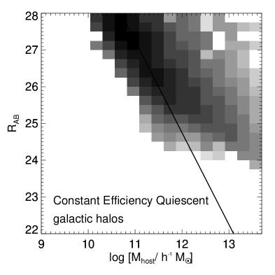
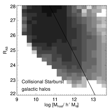
Figure 2: Joint probability distribution of extinction corrected observed ${\cal R}_{AB}$ magnitude and galactic halo mass (defined here as the halo the galaxy formed in — this is usually enclosed within another, larger halo, but may not be in the case of central galaxies), for the Constant Efficiency Quiescent (left) and Collisional Starburst (right) models. The shadings correspond to logarithmically spaced density bins, and the line indicates a linear relation between mass and luminosity.

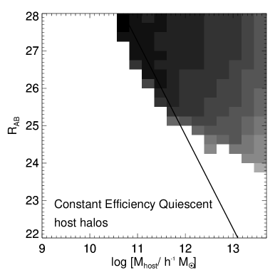
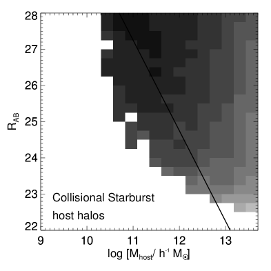
Figure 3: Joint probability distribution of extinction corrected observed-frame ${\cal R}_{AB}$ magnitude and host halo mass, for the Constant Efficiency Quiescent (left) and Collisional Starburst (right) models. The shadings correspond to logarithmically spaced density bins, and the line indicates a linear relation between mass and luminosity.

The relevant quantity for determining the correlation length, however, is the mass of the virialized host halo containing the galaxies. The joint distribution of galaxy magnitude and host halo mass is shown in Figure 3. This figure shows that in both models, massive halos can host a number of galaxies of varying luminosities. There is a critical luminosity, which reflects the brightest galaxy that can be produced in a halo of a given mass, and which is a fairly strong function of halo mass. The resulting weak dependence of luminosity on host halo mass, however, is not sufficient to produce a strong trend in the clustering strength with luminosity. The weak dependence of clustering on luminosity, which arises from a similar effect, has been noted before for galaxies at $z=0$ in semi-analytic models (Somerville et al. 2001).

Thus we argue that the weak dependence of clustering on luminosity is a generic feature of these types of hierarchical models, whether or not they include a bursting mode of star formation. Therefore, this test does not provide as strong a constraint on star formation modeling as we might have hoped, but rather is a reflection of the fact that significant sub-structure is present in halos.

We point out, however, that the scatter in the luminosity of objects versus the host mass is sensitive to the subhalo multiplicity function as determined by our semi-analytic models. If the number of low-mass subhalos per host were reduced, then the scatter in luminosity at fixed host mass would also be reduced, producing a stronger dependence of clustering on luminosity. Indeed, when the satellite multiplicity function from the semi-analytic models is compared with the subhalo multiplicity function obtained from the ART simulations discussed in §4.2.2, we find that, for a fixed circular velocity, the semi-analytic models produce a much larger number of subhalos per massive halo. This result may reflect the fact that the process of tidal disruption has been neglected in our semi-analytic treatment (see Bullock et al. 2000b). However, it is possible that the ART simulations could overestimate the severity of subhalo destruction, which might be reduced by the presence of condensed baryons (Katz et al. 1999 find that the correlation length of $z=3$ galaxies identified in their hydrodynamic simulations depends only very weakly on baryonic mass or number density, in agreement with our results). We defer a more detailed investigation of this issue to a later work (Wechsler 2001).

6 RELATING HALO COLLISIONS TO STARBURST GALAXIES

In §4.3, we showed the halo occupation number as a function of host halo mass for the Colliding Halo model and for the semi-analytic Collisional Starburst model. Although these two models represent the same physical scenario, i.e., one in which most bright galaxies at high redshift are the product of a collision-triggered burst of star formation, the results for the number of objects as a function of mass in the two models were quite different. If the number of objects is modeled by a power-law function of the mass of the host halo, we find that the slope of the occupation function for collisions identified in the simulation ($S\simeq 1.1$) is steeper than that of the observable galaxies produced in the semi-analytic Collisional Starburst model ($S=0.7$). In this section, we attempt to understand the source of this difference, and examine in detail the importance of various aspects of the recipe used to model starbursts in the semi-analytic model. This section is rather detailed, and may be skipped by the casual reader.

There are two possible causes for the discrepancy. Either the merger rate in the semi-analytic models disagrees with the merger rate measured from the simulations, or the difference is produced by the more detailed semi-analytic treatment of the luminosity of the burst resulting from each merger.

Clearly, one expects the simulations to do the most accurate job of properly identifying halo (and subhalo) collisions, at least above their resolution limit, because this is dependent solely on how matter interacts via gravity, which the simulation clearly represents more accurately than a semi-analytic model. However, it is possible that mergers below the resolution limit of the simulation could produce observable galaxies. Only halos with modeled mass of at least 50 particles ($6.25\times 10^{9}{h^{-1}}{\rm M}_{{}_{\mathord{\odot}}}$) are included in the halo catalog, and it is estimated to be 100% complete for masses above about $2\times 10^{10}{\rm M}_{{}_{\mathord{\odot}}}$ (Sigad et al. 2001).

The semi-analytic model can be run with arbitrarily high resolution; in practice the trees are truncated at halos with circular velocities of 40 km/s, which corresponds to a mass resolution of roughly $1\times 10^{8}{h^{-1}}{\rm M}_{{}_{\mathord{\odot}}}$ at $z=3$. The merger rate of galaxies (subhalos) is modeled using several approximations: extended Press–Schechter is used to construct the merger trees (Somerville & Kolatt 1999), and the merging of subhalos within virialized halos is modeled via the dynamical friction and modified mean free path approximations (see §4.2.3). Each of these approximations have been tested in isolation (see Kolatt et al. 2001 for a recent analysis), but it is unknown how accurately the merger rate produced by the whole machinery agrees with simulations. An additional concern is that the definition of what constitutes a merger may differ between the semi-analytic models and the simulations.

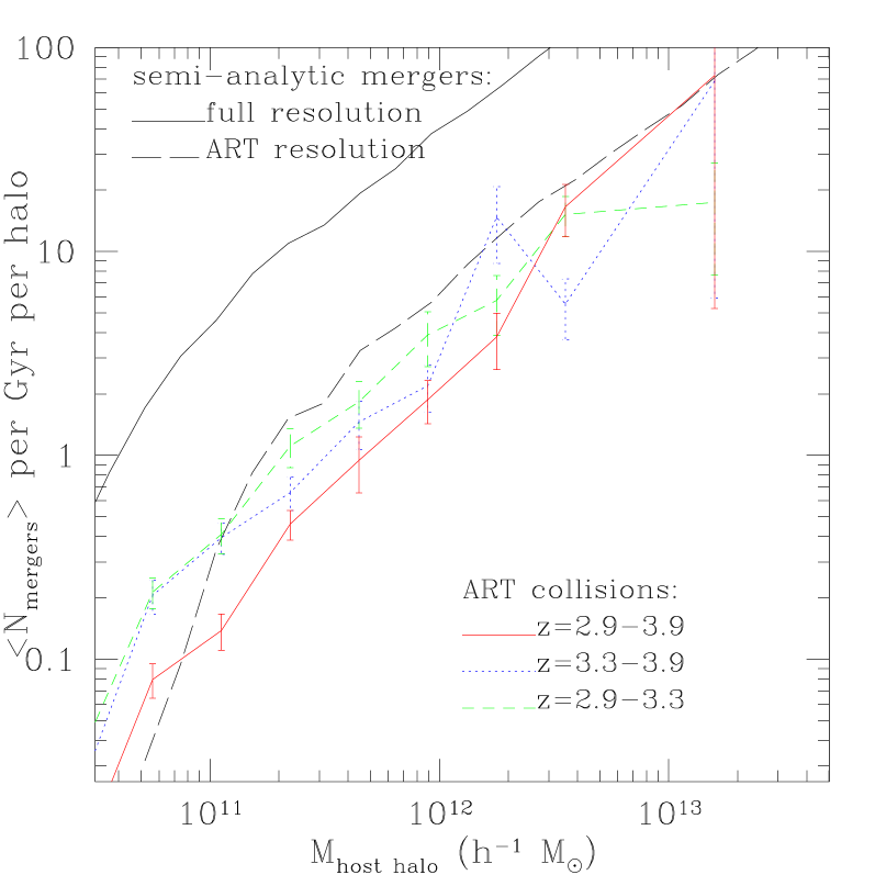
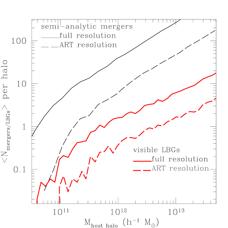
Figure 4: (Left) Average number of mergers per halo over the redshift interval $z=2.9-3.9$, as a function of host halo mass (see text for detailed definition), for the semi-analytic model and the ART simulation (includes unbound collisions). The dashed line shows only those mergers in the semi-analytic model for which each merging halo is above the resolution limit of the simulation; the solid line shows all the semi-analytic mergers. (Right) Average number of mergers per halo over the redshift interval $z=2.9-3.9$ in the semi-analytic model, and the average number of LBGs at $z=2.9$ in the CSB model (bold). Solid lines show all mergers at the full resolution of the semi-analytic model; dashed lines show only those mergers that would be identified with the resolution of the ART simulation.

In Figure 4 (left panel), the number of mergers per host halo as a function of the host mass measured in the ART simulations is compared with the same quantity estimated in the semi-analytic model. Both the total number of semi-analytic mergers and the semi-analytic mergers assuming the completeness function of the simulations (Sigad et al. 2001 are shown; the latter is equivalent to imposing the mass resolution of the simulation onto the semi-analytic models). In the simulations, all collisions that occur during some high-redshift timestep interval are identified, and assigned to the distinct (i.e., non-sub) “host” halos that they reside in at a later redshift. A similar thing is done for the semi-analytic model to make a comparison: we identify all mergers in the model that occur within the same timestep interval, and assign them to the host halo that they end up in at the end of the timestep. Although the actual number of mergers changes considerably as a function of assumed resolution in the semi-analytic models, the shape of the occupation function doesn’t change with resolution. We have also tested the effects of resolution directly by comparing the results of this simulation with the analysis of a larger box with 1/8 the mass resolution, and find a similar result. The semi-analytic results match the simulation within the (rather large) errors, although the slope is slightly shallower than the best-fit power-law from the simulation. The normalization is not entirely consistent, however, there are many possible reasons for this discrepancy — as has been discussed — and since the normalization is fixed for these models by comparison with observations and we are mainly concerned with the slope, this will not affect the results.

Inaccuracies in the merger rate built into the semi-analytic models therefore do not seem to be responsible for the discrepancy. We now examine the ingredients of the recipe for assigning luminosities to the mergers and determine how this affects the results. In Figure 4 (right panel), the two lines from the left panel of the figure are repeated, showing the number of mergers in the semi-analytic model over the redshift interval $2.9<z<3.9$, for the full resolution and with the ART resolution imposed. For comparison, we show on the same panel the number of LBGs that would be “observable” (as usual, defined here as galaxies with ${\cal R}_{AB}\leq 25.5$) in the semi-analytic model, both for the full resolution and for the case in which the model has the same resolution as the simulations. Two things are apparent: first, there are a large number of galaxies that would be bright enough to be included in our “Steidel-like” sample, and that are produced by mergers below the mass resolution of the ART simulation, and second, the resolution does not affect the slope of the occupation function for galaxies. The mergers in the semi-analytic model show a significantly steeper increase with host halo mass than the observable galaxies in the same model (virtually all of which were made bright by recent mergers), indicating that for some reason a collision is less likely to produce a bright galaxy if it occurs in a massive halo.

We now investigate which elements of the semi-analytic recipes produce this effect (Figure 6). First we consider a simple recipe for assigning luminosities to halo mergers, similar to that used in Kolatt et al. (1999). We assume that before each collision every galaxy has a cold gas reservoir that is a constant fraction of the (galactic) halo mass ($m_{\rm g}=f_{\rm g}f_{\rm b}m_{\rm halo}$, where $f_{\rm b}\equiv\Omega_{\rm b}\Omega^{-1}_{\rm m}$ is the fraction of mass in baryons and $f_{\rm g}$ is the fraction of baryons in cold gas). The mergers are divided into major ($m_{2}/m_{1}>0.25$) and minor mergers, and every collision is assumed to produces a burst of duration $\tau_{\rm burst}=50$ Myr, during which 75% and $50\%$ of the gas is converted into stars for major and minor mergers respectively. We assume that the mergers are uniformly distributed over the timestep. The apparent rest-1600 Å magnitude of each burst is estimated at the end of the timestep ($z=2.9$), using Bruzual-Charlot (GISSEL00) stellar-population synthesis models (assuming solar metallicity and a Salpeter initial mass function). This recipe ($f_{gas}$ = C, Kolatt et al. efficiency) is applied to the recorded mergers from the semi-analytic model. Comparing the resulting number of observable galaxies with the total number of mergers in Figure 6, we see that not all of the mergers produce observable galaxies, but the galaxy occupation function is actually even steeper than the mergers. This is not surprising, as we have assumed that a constant fraction of the halo mass is in the form of cold gas, so massive halos have more gas and are more likely to produce bright objects.

There are, however, a number of differences between this simple prescription and the full treatment of the semi-analytic model. The most relevant aspects and their treatment in the semi-analytic model are summarized below:

• Cold gas supply: depends on halo mass and collapse time, whether the galaxy is a central or satellite galaxy, and consumption by previous star formation and expulsion by supernovae feedback.

• Burst efficiency: modeled as a function of the mass ratio and morphology of the colliding galaxies. The efficiency of bursts in major mergers is nearly independent of morphology, but bursts in minor mergers are suppressed when a bulge is present.

• Burst timescale: modeled as equal to the dynamical time of the disk.

We discuss each of these in turn.

One can imagine that the more detailed modeling of the cold gas supply might go in the right direction. More massive halos have a much lower fraction of their mass in the form of cold gas, because the time for the gas to cool out to the virial radius is larger than a Hubble time. In addition, large halos will have many satellite galaxies, which are not allowed to receive any new gas from cooling, and therefore exhaust or expel their gas supply through star formation and supernovae winds. Both effects might lead to fainter bursts in massive halos because of a shortage of cold gas. To test this, for each merger in the semi-analytic model, we record the gas content of both progenitors. We now use this (SPF $f_{gas}$) instead of the constant gas fraction assumed above, but leave the other ingredients the same, and compute the number of observable galaxies as before. As is shown in Figure 6, some of the bursts in massive halos are suppressed by the gas supply effect, but the slope of the occupation function remains steeper than the full model in the largest mass host halos.

Average number of mergers per halo, from $z=2.9-3.9$ for the semi-analytic model, compared with galaxies with ${\cal R}_{AB}\leq 25.5$ (no dust correction) in the same model at $z=2.9$, where luminosities have been assigned using: a) the simple recipe of K99, b) same as a) but using the gas contents of the full CSB model, c) same as b) but using the bulge-fraction dependent burst efficiency function of SPF, and d) the actual CSB model.

Next we try the burst efficiency recipe of SPF (see Eqn. 10), including the dependence on the bulge fraction. Using this prescription, the occupation function for observable galaxies agrees fairly well with the results of the full model — at least the slope at the high-mass end is the same. The total number of galaxies is a bit smaller than in the full model, but this is perhaps to be expected as we have neglected quiescent star formation in this simple exercise. Note that in these models, bulges are built up by major mergers. Therefore it is not surprising that the massive halos, which formed from higher peaks in the initial density field, are more likely to contain galaxies with prominent bulges — this is just the high-redshift analog of the morphology-density relationship. The suppression of bursts in minor mergers for galaxies with existing bulges appears to be the main effect that flattens the LBG occupation function in the full model.

The effects investigated above seem to account for the differences between the simple Colliding Halo model and the full semi-analytic Collisional Starburst model, but this exercise has highlighted the sensitivity of our results to the detailed modeling of the efficiency and time dependence of star formation in the collisional starbursts, which remain highly uncertain. In particular, because minor mergers are so much more common than major mergers, the treatment of bursts in minor mergers is very important — yet it is also more sensitive to the details of the interaction. We are working to better understand these issues using a set of hydrodynamic simulations of colliding galaxies, similar to those of Mihos & Hernquist (1994), but with initial conditions chosen to be representative of $z\sim 3$ galaxies (Somerville et al. 2000a), and covering a larger parameter space.

7 DISCUSSION AND CONCLUSIONS

We have investigated a range of models, spanning the most extreme versions of previously proposed scenarios for Lyman-break galaxies, and compared the predicted clustering properties of galaxies at $z=3$ with those of Lyman-break galaxies with spectroscopic redshifts from the ground-based sample of Steidel, Adelberger, and collaborators. We investigated two simple models for assigning observable galaxies to halos, the Massive Halo model, which associates one LBGs with each massive halo, and the Colliding Halo model, which associates an LBG with each halo collision. In addition, we investigated three “realistic” models based on the semi-analytic models of SPF, which are differentiated by their assumptions about the efficiency of transforming cold gas into stars.

All five models are normalized to produce the observed, incompleteness corrected number density of LBGs (Steidel et al. 1999). For each model, we then compute the halo occupation function, or the number of observable galaxies per halo as a function of the host halo mass. These occupation functions are then used to populate dark-matter halos in a large, dissipationless $\Lambda$CDM N-body simulation with galaxies. We select galaxies, attempting to mimic the observational selection techniques, and then use the resulting catalogs to calculate the clustering properties of LBGs in each scenario.

Clustering statistics that smooth over a relatively large region (such as the overdensity distribution in cells of $\sim 12$ ${h^{-1}}$Mpc on a side, or the correlation length) are fairly non-discriminatory for all five models. No models can be strongly ruled out based on the correlation length; the most clustered is the Colliding Halo model, which is about $2\sigma$ away from the data. The correlation lengths for the rest of the models are in reasonable agreement with the data, when compared using the same technique. However, there is still uncertainty in the determination of the true correlation length of LBGs; if it is really closer to $3$ ${h^{-1}}$Mpc  rather than 4–5 ${h^{-1}}$Mpc, then this is probably an indication that LBGs must be hosted by smaller mass halos than any of our models predict. A change of a factor of two in the true number density of the objects seen as LBGs could possibly account for this. Alternatively, for the “realistic” models, the uncertainties in the modeling of star formation, feedback, and dust extinction, the stellar initial mass function, etc., are likely to be sufficient to allow for some adjustments that would change the occupation function in just the right way to satisfy all the constraints investigated here. One possibility, which we have not investigated in detail here, is that the most rapidly star-forming galaxies suffer so much dust extinction that they are not included in the observational sample. In this case, the proportion of visible galaxies in massive halos would be further reduced — thus lowering the correlation length. The hope, of course, is that the empirical understanding gained by this sort of schematic modeling will lead to constraints that will eventually bring about progress towards a deeper understanding of these physical processes.

The fraction of galaxies in close pairs, which is a good measure of the number of multiple galaxies in a single halo, proved to be a better discriminator between models than the statistics that measure clustering on larger scales. This is because this quantity is quite sensitive to the slope $S$ of the halo occupation function at the high mass end, $N_{g}\propto M^{S}$. This statistic can discriminate between the most extreme models, the simple Massive Halo model ($S=0$), which underproduces close pairs by more than $1\sigma$, and the Colliding Halo model ($S=1.1$), which overproduces them by several $\sigma$ (see Figure 5.3). The Collisional Starburst model, which has a halo occupation slope of $S\sim 0.7$ produces good agreement with the close pair fraction of the observations; the other two “realistic” semi-analytic models yield a slightly higher slope of $S\sim 0.8$, and a higher fraction of pairs than the data, but are not strongly ruled out by the current data.

We also examined the dependence of clustering on luminosity. There have been suggestions that the correlation length derived from the observations depends on the magnitude limit of the sample, with brighter galaxies being more strongly clustered (S98, G00). This has been interpreted as evidence for a tight connection between halo mass and galaxy luminosity, which would seem to disfavor models with stochastic star formation such as collisional starbursts. However, when all available measurements of the correlation length from the literature are compiled, it seems clear that the strength of this observational trend depends greatly on which subset of the observations one chooses to include. Until a single high-redshift sample exists that is large enough in volume to measure the clustering of bright galaxies without being dominated by shot-noise, and deep enough to simultaneously measure the clustering of much fainter galaxies, it will be difficult to place strong limits on the models.

In the meantime, for the models, we find that both the quiescent and collisional starburst models display only a weak trend of correlation length with luminosity, much weaker than that suggested by the observational analysis of G00, or predicted by the Massive Halo model. As expected, the relation between galaxy luminosity and halo mass has much larger scatter in starburst models than in quiescent models. However, since massive halos can have a number of subhalos, with a variety of masses, both models actually have quite a large scatter in the luminosities of galaxies that reside in these host halos, which are what determine the clustering properties.

Any hierarchical clustering model will have multiple subhalos within the massive halos, with a range of masses, several of which are likely to correspond to observable galaxies. In fact, the observed fraction of galaxies in close pairs seems to indicate that many of the halos do host more than one visible galaxy, since the number of pairs in the Massive Halo model is more than $1\sigma$ lower than the data (the first bin in Figure 5.3). It is a concern that there is some disagreement between the subhalo multiplicity function of the semi-analytic models compared to that in the simulations; if in fact the number of subhalos predicted by the semi-analytic treatment is too high, the dependence of clustering on luminosity would be somewhat stronger.

We found that two versions of the collisional starburst scenario gave different results for the halo occupation function and tried to understand why. The Colliding Halo model, based on properties of collisions identified in high-resolution N-body simulations, had many more LBGs in massive halos than the semi-analytic model, and a steeper halo occupation function. Although the difference could have been caused by an inaccurate treatment of halo mergers in the semi-analytic analysis, we found that this was not the case. Instead, the discrepancy between this model and the semi-analytic Collisional Starburst model arises because of the detailed modeling of gas processes and starburst efficiency in the latter. Namely, high-mass halos in the semi-analytic model are less efficient at producing bright galaxies. This is primarily due to two effects: massive halos collapse more recently and have not had time to cool as large a fraction of their gas, and (the more dominant effect) bursts in minor mergers are suppressed when the primary galaxy already contains a prominent bulge. This recipe was adopted by SPF to attempt to capture the behavior found by Mihos & Hernquist (1996), based on hydrodynamic simulations of merging galaxies. Apparently, a morphology-density relation is already in place in our models at $z\sim 3$, and this has a significant impact on the predicted properties of observable galaxies. It should be noted that although SPF based their recipe for burst efficiency on the best simulations that were available at the time, the sensitivity of our results to this ingredient is a concern. A more extensive set of simulations, with initial conditions chosen to better represent $z\sim 3$ galaxies and covering a larger region of parameter space, is in progress (Somerville et al. 2000a) and will hopefully improve our understanding of this process. In the meantime, one should be aware that the predictions for clustering in this model are especially sensitive to the assumed efficiency of converting gas into stars during a starburst.

In summary, although one might have expected the clustering properties of galaxies on intermediate scales (i.e., the correlation length) to provide a strong discriminator between models of galaxy formation, in fact we find that even extreme models yield similar results for this statistic — although models with a very steep occupation function are only marginally acceptable. Clustering statistics that probe smaller scales are a better way to discriminate between models whose halo occupation slopes are different, but even with this statistic, none of the more realistic models can be strongly ruled out with the data sample used here. Interestingly, we found that the halo occupation slope was shallower in the Collisional Starburst model than in the massive quiescent models investigated, laying to rest concerns that this model would comparatively have too many close pairs. When combined with the failings of the other two (quiescent) models discussed in SPF, it still appears that the Collisional Starburst provides the best agreement with all the available data. Still, we emphasize that many ingredients of the modeling of collisional starbursts remain highly uncertain, and if indeed this process is responsible for producing most of the galaxies observed at high redshift, further investigation will be crucial. It should also be emphasized that although the current observational situation is still too uncertain to unambiguously determine how these high-redshift galaxies are related to the underlying dark halos, there is hope that in the future, a combination of observations on number density, and both small-scale and large-scale clustering, should be able to determine the halo occupation function, which we then can hope to explain with physical models for galaxy formation.

8 ACKNOWLEDGMENTS

We thank Kurt Adelberger for help with interpreting the data, for providing some data in electronic form, and for several useful discussions throughout the course of this project. We also thank Sandy Faber, Mauro Giavalisco, Lars Hernquist, Patrik Jonsson, and Ari Maller for useful discussions and comments. We would also like to thank Andrey Kravtsov & Anatoly Klypin for running and providing access to the ART simulations, which were run at NSCA and NRL, and the GIF collaboration for providing access to their simulations. RHW has received support from a NSF GAANN fellowship at UCSC. JRP acknowledges a Humboldt Award at the Max Planck Institute for Physics in Munich. JSB received support from NASA LTSA grant NAG5-3525 and NSF grant AST-9802568. This work was also supported by a NASA ATP grant, NSF grants AST-9529098 and PHY-9722146, and a Faculty Research Grant at UCSC, and by the US-Israel Binational Science Foundation grant 98-00217 and Israel Science Foundation grant 546/98. We also acknowledge the hospitality of the Institute for Theoretical Physics at UC Santa Barbara, and RHW acknowledges the hospitality of the Hebrew University of Jerusalem, the IoA, Cambridge, and the Max Planck Institute for Astrophysics, Garching.

References

- Adelberger (2000) Adelberger, K. L. 2000, in ASP Conference Series, Vol. 200, Clustering at High Redshift, ed. A. Mazure, O. Le Fevre, & V. Le Brun (Kluwer Academic Publishers)
- Adelberger & Steidel (2000) Adelberger, K. L. & Steidel, C. C. 2000, ApJ, 544, 218
- Adelberger et al. (1998) Adelberger, K. L., Steidel, C. C., Giavalisco, M., Dickinson, M., Pettini, M., & Kellogg, M. 1998, ApJ, 505, 18, (A98)
- Adelberger et al. (2001) —. 2001, in preparation
- Arnouts et al. (1999) Arnouts, S., Cristiani, S., Moscardini, L., Matarrese, S., Lucchin, F., Fontana, A., & Giallongo, E. 1999, MNRAS, 310, 540
- Bagla (1998) Bagla, J. S. 1998, MNRAS, 297, 251
- Baugh et al. (1999) Baugh, C. M., Benson, A. J., Cole, S., Frenk, C. S., & Lacey, C. G. 1999, MNRAS, 305, L21
- Baugh et al. (1998) Baugh, C. M., Cole, S., Frenk, C. S., & Lacey, C. G. 1998, ApJ, 498, 504
- Benson et al. (2000) Benson, A. J., Cole, S., Frenk, C. S., Baugh, C. M., & Lacey, C. G. 2000, MNRAS, 311, 793
- Blanton et al. (2000) Blanton, M., Cen, R., Ostriker, J., Strauss, M., & Tegmark, M. 2000, ApJ, 531, 1
- Bullock et al. (2000a) Bullock, J. S., Kolatt, T. S., Sigad, Y., Somerville, R. S., Kravtsov, A. V., Klypin, A. A., Primack, J. R., & Dekel, A. 2000a, MNRAS, 321, 559
- Bullock et al. (2000b) Bullock, J. S., Kravtsov, A. V., & Weinberg, D. 2000b, ApJ, 539, 517
- Cole et al. (1994) Cole, S., Aragón-Salamanca, A., Frenk, C., Navarro, J., & Zepf, S. 1994, MNRAS, 271, 781
- Coles et al. (1998) Coles, P., Lucchin, F., Matarrese, S., & Moscardini, L. 1998, MNRAS, 300, 183
- Gardner et al. (1999) Gardner, J., Katz, N., Hernquist, L., & Weinberg, D. 1999, ApJ, submitted (astro-ph/9911343)
- Giavalisco & Dickinson (2001) Giavalisco, M. & Dickinson, M. E. 2001, ApJ, in press (astro-ph/0012249, G00)
- Giavalisco et al. (1998) Giavalisco, M., Steidel, C. C., Adelberger, K. L., Dickinson, M. E., Pettini, M., & Kellogg, M. 1998, ApJ, 503, 543, (G98)
- Governato et al. (1998) Governato, F., Baugh, C. M., Frenk, C. S., Cole, S., Lacey, C. G., Quinn, T., & Stadel, J. 1998, Nature, 392, 359
- Haiman & Hui (2001) Haiman, Z. & Hui, L. 2001, ApJ, in press (astro-ph/0002190)
- Jenkins et al. (1998) Jenkins, A., Frenk, C. S., Pearce, F. R., Thomas, P. A., Colberg, J. M., White, S. D. M., Couchman, H. M. P., Peacock, J. A., Efstathiou, G., & Nelson, A. H. 1998, ApJ, 499, 20
- Jing (1999) Jing, Y. P. 1999, ApJ, 515, L45
- Jing & Suto (1998) Jing, Y. P. & Suto, Y. 1998, ApJ, 494, L5
- Katz et al. (1999) Katz, N., Hernquist, L., & Weinberg, D. H. 1999, ApJ, 523, 463
- Kauffmann et al. (1999a) Kauffmann, G., Colberg, J. M., Diaferio, A., & White, S. D. M. 1999a, MNRAS, 303, 188
- Kauffmann et al. (1999b) —. 1999b, MNRAS, 307, 529
- Kauffmann et al. (1997) Kauffmann, G., Nusser, A., & Steinmetz, M. 1997, MNRAS, 286, 795
- Kennicutt (1998) Kennicutt, R. C. 1998, ApJ, 498, 541
- Kolatt et al. (2001) Kolatt, T., Bullock, J., Sigad, Y., Primack, J., Dekel, A., Kravtsov, A., & Klypin, A. 2001, MNRAS, submitted (astro-ph/0010222)
- Kolatt et al. (1999) Kolatt, T. S., Bullock, J. S., Somerville, R. S., Sigad, Y., Jonsson, P., Kravtsov, A. V., Klypin, A. A., Primack, J. R., Faber, S. M., & Dekel, A. 1999, ApJ, 523, L109, (K99)
- Kravtsov et al. (1997) Kravtsov, A. V., Klypin, A. A., & Khokhlov, A. M. 1997, ApJS, 111, 73
- Kuiper (1962) Kuiper, N. H. 1962, in Proceedings of the Korinklijke Nederlandse Akademie van Wetenschappen, ser. A, Vol. 63, 38–47
- Lacey & Cole (1993) Lacey, C. & Cole, S. 1993, MNRAS, 262, 627
- Lowenthal et al. (1997) Lowenthal, J. D., Koo, D. C., Guzman, R., Gallego, J., Phillips, A. C., Faber, S. M., Vogt, N. P., Illingworth, G. D., & Gronwall, C. 1997, ApJ, 481, 673
- Madau et al. (1996) Madau, P., Ferguson, H., Dickinson, M., Giavalisco, M., Steidel, C., & Fruchter, A. 1996, MNRAS, 283, 1388
- Magliocchetti & Maddox (1999) Magliocchetti, M. & Maddox, S. J. 1999, MNRAS, 306, 988
- Makino & Hut (1997) Makino, J. & Hut, P. 1997, ApJ, 481, 83
- Martini & Weinberg (2001) Martini, P. & Weinberg, D. 2001, ApJ, in press (astro-ph/0002384)
- Mihos & Hernquist (1994) Mihos, J. & Hernquist, L. 1994, ApJ, 425, L13
- Mihos & Hernquist (1995) —. 1995, ApJ, 448, 41
- Mihos & Hernquist (1996) —. 1996, ApJ, 464, 641
- Mo & Fukugita (1996) Mo, H. J. & Fukugita, M. 1996, ApJ, 467, L9
- Mo et al. (1999) Mo, H. J., Mao, S., & White, S. D. M. 1999, MNRAS, 304, 175
- Mo & White (1996) Mo, H. J. & White, S. D. M. 1996, MNRAS, 282, 347
- Moscardini et al. (1998) Moscardini, L., Coles, P., Lucchin, F., & Matarrese, S. 1998, MNRAS, 299, 95
- Peebles (1980) Peebles, P. J. E. 1980, The Large-Scale Structure of the Universe (Princeton University Press)
- Press & Schechter (1974) Press, W. H. & Schechter, P. 1974, ApJ, 187, 425
- Press et al. (1992) Press, W. H., Teukolsky, S. A., Vetterling, W. T., & Flannery, B. P. 1992, Numerical Recipes in C (Cambridge University Press)
- Sheth & Tormen (1999) Sheth, R. K. & Tormen, G. 1999, MNRAS, 308, 119
- Sigad et al. (2001) Sigad, Y., Kolatt, T., Bullock, J., Kravtsov, A. V., Klypin, A. A., Primack, J. R., & Dekel, A. 2001, MNRAS, submitted (astro-ph/0005323)
- Somerville (1997) Somerville, R. 1997, PhD thesis, University of California, Santa Cruz
- Somerville & Kolatt (1999) Somerville, R. S. & Kolatt, T. S. 1999, MNRAS, 305, 1
- Somerville et al. (2000a) Somerville, R. S., Lemson, G., Kolatt, T. S., & Dekel, A. 2000a, MNRAS, 316, 479
- Somerville et al. (2001) Somerville, R. S., Lemson, G., Sigad, Y., Dekel, A., Kauffmann, G., & White, S. 2001, MNRAS, 320, 289
- Somerville et al. (2000b) Somerville, R. S., Primack, J. R., & Faber, S. M. 2000b, MNRAS, in press, (SPF)
- Spinrad et al. (1998) Spinrad, H., Stern, D., Bunker, A., Dey, A., Lanzetta, K., Yahil, A., Pascarelle, S., & Fernandez-Soto, A. 1998, AJ, 116, 2617
- Steidel et al. (1998) Steidel, C., Adelberger, K., Giavalisco, M., Dickinson, M., Pettini, M., & Kellogg, M. 1998, in Royal Society Discussion Meeting, ”Large Scale Structure in the Universe”, (astro-ph/9805267, S98)
- Steidel et al. (1996a) Steidel, C., Giavalisco, M., Dickinson, M., & Adelberger, K. 1996a, AJ, 112, 352
- Steidel et al. (1996b) Steidel, C., Giavalisco, M., Pettini, M., Dickinson, M., & Adelberger, K. 1996b, ApJ, 462, L17
- Steidel & Hamilton (1992) Steidel, C. & Hamilton, D. 1992, AJ, 104, 941
- Steidel et al. (1999) Steidel, C. C., Adelberger, K. L., Giavalisco, M., Dickinson, M., & Pettini, M. 1999, ApJ, 519, 1
- Wang & Heckman (1996) Wang, B. & Heckman, T. M. 1996, ApJ, 457, 645
- Wechsler (2001) Wechsler, R. H. 2001, PhD thesis, University of California, Santa Cruz
- Wechsler et al. (1998) Wechsler, R. H., Gross, M. A. K., Primack, J. R., Blumenthal, G. R., & Dekel, A. 1998, ApJ, 506, 19
- Weinberg et al. (2000) Weinberg, D., Hernquist, L., & Katz, N. 2000, ApJ, submitted (astro-ph/0005340)
- Weymann et al. (1998) Weymann, R., Stern, D., Bunker, A., Spinrad, H., Chaffee, F., Thompson, R., & Storrie-Lombardi, L. 1998, ApJ, 505, L95