On the dependence of spectroscopic indices of early-type galaxies on age, metallicity and velocity dispersion

Abstract

We investigate the Mg–$\sigma$ and $<$Fe$>$–$\sigma$ relations in a sample of 72 early-type galaxies drawn mostly from cluster and group environments using a homogeneous data-set which is well-calibrated onto the Lick/IDS system. The small intrinsic scatter in Mg at a given $\sigma$ gives upper limits on the spread in age and metallicity of $49$% and $32$% respectively, if the spread is attributed to one quantity only and if the variations in age and metallicity are uncorrelated. The age/metallicity distribution as inferred from the ${\mathrm{H}}\beta$ vs $<$Fe$>$ diagnostic diagram reinforces this conclusion, as we find mostly galaxies with large luminosity weighted ages spanning a range in metallicity. Using Monte-Carlo simulations, we show that the galaxy distribution in the ${\mathrm{H}}\beta$ vs $<$Fe$>$ plane cannot be reproduced by a model in which galaxy age is the only parameter driving the index-$\sigma$ relation. In our sample we do not find significant evidence for an anti-correlation of ages and metallicities which would keep the index–$\sigma$ relations tight while hiding a large spread in age and metallicity. As a result of correlated errors in the age-metallicity plane, a mild age-metallicity anti-correlation cannot be completely ruled out given the current data. Correcting the line-strengths indices for non-solar abundance ratios following the recent paper by Trager et al., leads to higher mean metallicity and slightly younger age estimates while preserving the metallicity sequence. The [Mg/Fe] ratio is mildly correlated with the central velocity dispersion and ranges from [Mg/Fe] $=$ 0.05 to 0.3 for galaxies with $\sigma>100$ km s^-1. Under the assumption that there is no age gradient along the index–$\sigma$ relations, the abundance-ratio corrected Mg–$\sigma$, Fe–$\sigma$ and ${\mathrm{H}}\beta$–$\sigma$ relations give consistent estimates of $\Delta{\mathrm{[}M/H]}/\Delta\log\sigma\simeq 0.9\pm 0.1$. The slope of the ${\mathrm{H}}\beta$–$\sigma$ relation limits a potential age trend as a function of $\sigma$ to 2-3 Gyrs along the sequence.

1 INTRODUCTION

Over the last two decades spectroscopic and photometric observations of nearby early-type galaxies have shown that they obey tight scaling relations. For example more luminous galaxies are redder [Sandage & Visvanathan 1978, Larson, Tinsley & Caldwell 1980, Bower, Lucey & Ellis 1992]; the strength of the Mg-absorption (at $\sim$5175 Å) increases with increasing central velocity dispersion [Terlevich et al. 1981, Bender, Burstein & Faber 1993, Colless et al. 1999]; and early-type galaxies populate only a band (or ‘plane’) in the three dimensional space of central velocity dispersion, effective radius, and mean effective surface brightness, the so called ‘Fundamental Plane’ [Djorgovski & Davis 1987, Dressler et al. 1987].

The tightness of the scaling relations has traditionally been interpreted as evidence for a very homogeneous population of early-type galaxies, i.e., old stellar populations and similar dynamical make-up of the galaxies [Bower, Lucey & Ellis 1992, Renzini & Ciotti 1993, Ellis et al. 1997, van Dokkum et al. 1998]. For example the colour-magnitude relation is perhaps best explained by a correlation of the metal abundance of the stellar population and total galaxy mass with no age gradient along the sequence [Bower, Lucey & Ellis 1992, Kodama et al. 1998, Vazdekis et al. 2000]. However, evidence is being found that elliptical galaxies do generally have complicated dynamical structures (e.g., decoupled cores) and disturbed morphologies (e.g., shells), suggesting an extended and complex assembly such as in a hierarchical merging picture (e.g., Cole et al. 2000). Furthermore measurements of absorption line-strength indices together with evolutionary population synthesis models suggest that the mean age of the stellar populations in early-type galaxies span a wide range [González 1993, Trager et al. 1998].

There is a hint of a connection between the detailed morphology and the mean ages of the stellar populations as ellipticals with disky isophotes show on average younger ages [de Jong & Davies 1997, Trager 1997]. This is in agreement with the studies of cluster galaxies at modest look-back times of 3-5 Gyr where an increased fraction of blue, late-type galaxies is found [Butcher & Oemler 1978, Butcher & Oemler 1984]. Probably this change is associated with the transformation of spiral galaxies into S0 types observed over the same interval [Dressler, et al. 1997, Couch et al. 1998]. How can we reconcile the existence of tight scaling relations for present day early-type galaxies with the evidence of an extended galaxy assembly and star formation history? An answer to this question rests largely on our understanding of the detailed physical processes which determine the spectral or photometric properties seen in scaling relations.

Broad band colours and line-strength indices of integrated stellar populations are sensitive to changes in both their age and metallicity. In fact it is possible to find many different combinations of ages and metallicities which produce similar overall photometric properties (age-metallicity degeneracy, Worthey 1994). In order to explain tight scaling relations, despite the presence of a substantial diversity in the integrated stellar populations, it has been suggested that the ages and metallicities of integrated stellar populations ‘conspire’ such that deviations from a given scaling relation due to age variations are balanced by an appropriate change in metallicity and vice versa; e.g., an age-metallicity anti-correlation [Trager et al. 1998, Ferreras, Charlot & Silk 1999, Trager et al. 2000b]. For example, a re-analysis of the González sample by Trager et al. appears to show that galaxies with a young stellar component are also more metal rich. Recently, evidence for a negative age-metallicity correlation has also been found in other data sets [Jørgensen 1999] and in literature compilations [Terlevich & Forbes 2000]. In contrast to this Kuntschner & Davies (1998) and Kuntschner (2000) did not find strong evidence for the existence of an age-metallicity anti-correlation in their analysis of the Fornax cluster. However, to date there is a lack of large, high quality samples with which it would be possible to probe the population of early-type galaxies as a whole.

In this paper we seek to further our understanding of scaling relations such as Mg–$\sigma$. We investigate the spread in the mean ages and metallicities at a given mass but also probe the possibility of age and metallicity trends along the relations. We use established methods such as the analysis of the scatter [Colless et al. 1999] in the Mg–$\sigma$ relation and line-strength age/metallicity diagnostic diagrams, and take advantage of recent advances in stellar population modeling such as improved corrections for non-solar abundance ratios [Trager et al. 2000a]. We employ a homogeneous and high-quality subset of the data collected initially for the SMAC peculiar motion survey [Hudson et al. 1999, Smith et al. 2000]. The sample is not complete but includes galaxies drawn mostly from nearby clusters and groups with some galaxies from less dense environments.

The present paper is organized as follows. Section 2 describes the sample selection, observations, data reduction and the measurements of the line-strength indices. Section 3 presents the Mg–$\sigma$ and Fe–$\sigma$ relations with an initial investigation into the scatter and slopes. In Section 4 we present a detailed analysis of age-metallicity diagnostic diagrams including an improved treatment of non-solar abundance ratios. The effects of the non-solar abundance ratio corrections on the age-metallicity estimates and on the index–$\sigma$ relations are presented in Sections 5 and 6 respectively. Our conclusions are given in Section 7.

2 OBSERVATIONS

2.1 Sample Description

The data reported here is from the SMAC I97MA spectroscopic run (see Smith et al. 2000 for further details). This run was undertaken principally to provide a secure connection of the SMAC data to other data sets and concentrated on observing galaxies with measurements previously reported by Dressler (1984), González (1993) and Davies et al. (1987). Accordingly the SMAC I97MA data shows a good overlap with the Lick/IDS system with 48 galaxies in common. In selecting targets, higher priority was given to galaxies with measurements from multiple sources. While the sample is dominated by ellipticals in the Virgo and Coma clusters, it does include a few S0s and galaxies in less dense environments (see Table 5 of the Appendix). It is not a complete sample in any sense and our sensitivity to environmental effects is limited. However, we did not find strong differences between galaxies from different environments or morphologies in our sample and thus throughout this paper we do not split up our sample but treat it as a whole.

2.2 Observations and Data Reduction

The observations were carried out by JRL at the 2.5m Isaac Newton Telescope (March 1997). The Intermediate Dispersion Spectrograph was used in conjunction with the 23.5cm camera, the 900V grating and a Tek1K chip. With a slit width of 3 arcsec, an instrumental resolution of $\sim 4$ Å FWHM was achieved, equivalent to an instrumental dispersion ($\sigma_{\rm instr}$) of 98 km s^-1. The spectra cover a wavelength range of 1024 Å, sampled at 1 Å pix^-1 from 4800 to 5824 Å. In total 200 galaxy spectra were obtained including many repeat observations. Along the slit the central five pixels of each observation were combined giving an effective aperture of $3.0\times 3.4$ arcsec². For other basic data reduction details and the velocity dispersion measurements see Smith et al. (2000).

The wavelength range and the redshift distribution of our data allows the measurement of five important line-strength indices (${\mathrm{H}}\beta$, Mg₂, Mg b, Fe5270, Fe5335) in the Lick/IDS system (Worthey 1994, hereafter W94, Trager et al. 1998). The indices were measured on the galaxy spectra after they had been corrected to a relative flux scale and were broadened to the Lick/IDS resolution (see also Worthey & Ottaviani 1997). The index measurements were then corrected for internal velocity broadening of the galaxies following the method outlined in Kuntschner (2000). The formal measurement errors were rescaled to ensure agreement with the error estimates derived from the repeat observations (the scale factors ranged from 0.80 to 1.07 for all indices but Mg₂ with a scale factor of 0.44). In order to maximize the S/N, multiple index measurements of the same galaxy were averaged giving a sample of 140 different galaxies. The effective S/N per Å of these combined measurements ranges from 14 to 78. In order to keep the errors of the index measurements reasonably low we decided to use only index measurements with an effective $\mathrm{S/N}\geq 30$ per Å giving a final sample of 72 galaxies (median S/N $\sim 40$ per Å) which we will analyze in this paper.

All of our data were obtained using the same physical aperture size, but since the galaxies span a factor of $\sim$10 in distance, the spectra sample different physical aperture sizes in kpc. Since line indices and velocity dispersion exhibit measurable gradients with respect to radius, it is necessary to correct these parameters to a ‘standard’ aperture. Here we adopt a generalisation of the aperture correction due to Jørgensen, Franx & Kjærgaard (1995), which scales parameters to a circular aperture of diameter 1.19 $h^{-1}$ kpc, $H_{0}=100~{}h~{}$km s^-1 Mpc^-1, equivalent to a circular aperture of 3.4 arcsec at the distance of Coma. The strength of the correction (i.e., the correction in the quantity per dex in aperture size) is $-0.04$ for $\log\sigma$, Mg₂ and Mg b, but $-0.02$ for $<$Fe$>$ and zero (i.e., no correction) for ${\mathrm{H}}\beta$. These correction strengths are based on the average line strength gradients observed in early-type galaxies [Kuntschner 1998]. The correction strengths adopted in this paper are overall similar to the ones used in Jørgensen (1997), however we use $-0.02$ for the $<$Fe$>$ index, whereas Jørgensen used $-0.05$.

2.3 Matching the Lick/IDS system

In order to determine the systematic offsets between our line-strength system and the original Lick/IDS system (on which the Worthey 1994 model predictions are based), we compared index measurements for the 48 galaxies in common with the Lick galaxy library [Trager et al. 1998]. We note that the Lick/IDS aperture was $1.4\times 4$ arcsec; so for the following comparison our data was corrected to the (fixed) Lick/IDS aperture using the formula given in Jørgensen et al. (1995).

Generally there is good agreement between the two data sets and only small offsets are found (see Table 1 and Figure 1). In order to match the Lick/IDS system we removed the offsets from our data. The median measurement errors in the indices, for our sample galaxies, are given in column 4 of Table 1. For a definition of non-standard line-strength indices see Section 2.5.

Table 1: Lick/IDS offsets and median index errors

Index	(Lick/IDS – this data)		index error	units
H$\beta$	$-0.11\pm 0.04$	(0.28)	0.17	Å
Mg2	$0.007\pm 0.002$	(0.014)	0.005	mag
Mg b	$-0.06\pm 0.05$	(0.36)	0.18	Å
$<$Fe$>$	$-0.08\pm 0.04$	(0.29)	0.16	Å
Mg b ′	–		0.007	mag
$<\mathrm{Fe}\,^{\prime}\negthinspace>$	–		0.004	mag
[OIII]$\lambda 5007$	–		0.10	Å
$\sigma_{0}$	–		0.014	dex

Note: There are 48 galaxies in common between the Lick/IDS sample and our data set. The quoted offset errors (column 2) reflect the error on the mean offset. The rms scatter is given in brackets. Column 4 lists the median index error for all indices used in this paper.

2.4 Comparison with other studies

We can compare our Lick/IDS-corrected data with the galaxies in common with González (1993), Jørgensen (1999) and Mehlert et al. (2000). Note, that the former authors also corrected their indices onto the Lick/IDS system. Any aperture differences were corrected following Jørgensen et al. (1995) and Jørgensen (1997).

For the Mg b and $<$Fe$>$ indices there is good general agreement between our data and the literature (see Table 2 and Figure 1) with offsets $\leq 0.1$ Å. We also find good agreement between our data and González for the ${\mathrm{H}}\beta$ index. The Mehlert et al. data compares less favourably with an offset of 0.19 Å, while the comparison with Jørgensen shows a large offset of 0.33 Å. The offset with respect to Jørgensen is difficult to interpret, since her data was also calibrated to the Lick/IDS system. While Jørgensen’s spectra were obtained with two different instruments (LCS and FMOS), both data sets show the same offset. The data points plotted in Figure 1 show the combined data sets of Jørgensen. She also measured a variant of the ${\mathrm{H}}\beta$ index, the so-called H$\beta_{G}$ index (defined in Jørgensen 1997). This index is not part of the original Lick/IDS system but has the advantage of smaller errors compared to ${\mathrm{H}}\beta$ at the same S/N. A comparison for this index shows a much better agreement between our data and Jørgensen’s (see Figure 2) with an offset of only 0.1 Å and a small rms scatter of 0.12 Å. While we do not have an explanation for the disagreement with Jørgensen, we conclude that our index measurements are well calibrated onto the Lick/IDS system with a systematic error $\leq 0.1$ Å.

Table 2: Offsets to literature data

Index	Lick – this data	González – this data	Jørgensen – this data	Mehlert et al. – this data
H$\beta$	0.00 $\pm$0.04 (0.28) Å	+0.09 $\pm$0.04 (0.16) Å	+0.33 $\pm$0.06 (0.24) Å	+0.19 $\pm$0.06 (0.23) Å
H$\beta_{G}$	–	–	+0.10 $\pm$0.03 (0.12) Å	–
Mg b	0.00 $\pm$0.05 (0.36) Å	–0.03 $\pm$0.04 (0.17) Å	+0.07 $\pm$0.06 (0.26) Å	–0.08 $\pm$0.06 (0.20) Å
$<$Fe$>$	0.00 $\pm$0.04 (0.29) Å	+0.06 $\pm$0.05 (0.18) Å	+0.03 $\pm$0.06 (0.27) Å	–0.05 $\pm$0.07 (0.25) Å
# of galaxies	48	17	19 (15 for H$\beta$ & H$\beta_{G}$)	14

Note: For the comparison shown here with the Lick data (Trager et al. 1998), González (1993), Jørgensen (1999) and Mehlert et al. (2000) our data was corrected for the Lick/IDS offset as summarized in Table 1. Errors on the mean offset are given. The rms scatter is given in brackets. The number of galaxies in common with each dataset from the literature is given in the last row.

Figure 1: Comparisons of our line-strength measurements with the literature (Lick data; Trager et al. 1998, González 1993, Jørgensen 1999 and Mehlert et al. 2000) for the Mg b, $<$Fe$>$ and ${\mathrm{H}}\beta$ indices. Our data was corrected for the Lick/IDS offset prior to comparison. The offsets to the data sets of González(1993), Jørgensen (1999) and Mehlert et al. (2000) are summarized in Table 2. All indices are measured in Å.

Figure 2: Comparisons of our line-strength measurements of H$\beta_{G}$ with the 15 galaxies in common with Jørgensen (1999). The mean offset is 0.1 Å (Jørgensen – this data) with a rms scatter of 0.12 Å.

The Smith et al. velocity dispersion measurements have been transformed onto the SMAC standard system by adding the correction $\Delta\log\sigma=-0.0084\pm 0.0046$, determined by Hudson et al. (2000) from simultaneous comparisons of many data sources. This correction is negligibly small for the purposes of this paper.

Our fully corrected line-strength and central velocity dispersion measurements used in this study are summarized in Table 5 of the Appendix.

2.5 Special indices

For the line-strength analysis in this paper we will use a Fe indicator which is the mean of the Lick Fe5270 and Fe5335 indices in order to suppress measurement errors [Gorgas, Efstathiou & Aragon-Salamanca 1990]:

$$<{\mathrm{F}e}>=({\mathrm{F}e5270}+{\mathrm{F}e5335})/2$$ (1)

Furthermore, following the papers by Colless et al. (1999), Smith et al. (2000) and Kuntschner (2000) we will sometimes express the line-strengths in magnitudes of absorbed flux, indicating this usage by a prime after the index (e.g., Mg b ^′)

$${\mathrm{i}ndex}\,^{\prime}=-2.5\log\left(1-\frac{\mathrm{i}ndex}{\Delta\lambda}\right)$$ (2)

where $\Delta\lambda$ is the width of the index bandpass. For $<$Fe$>$ we define $<\mathrm{Fe}\,^{\prime}\negthinspace>$ = (Fe5270 ^′ + Fe5335 ^′)/2. Note, that the Mg₂ index is always expressed in magnitudes.

In order to estimate the amount of nebular emission present in galaxies, we defined a [OIII]$\lambda 5007$ index similar to the other Lick/IDS indices, with continuum passbands of 4978–4998 Å and 5015–5030 Å and a central passband of 4998–5015 Å. Our measurements of the [OIII]$\lambda 5007$ emission were then compared with the González (1993) measurements for the 17 galaxies in common. The agreement between our measurements and González’s is excellent (see Figure 3). We note, that González measured the [OIII]$\lambda 5007$ emission after subtracting the spectrum of the host galaxy whereas our [OIII]$\lambda 5007$ index was measured directly on the spectra, leading to an effective absorption measurement when no emission is present. In order to transform our [OIII]$\lambda 5007$ index measurements into estimates of the true [OIII]$\lambda 5007$ emission we subtracted an offset of 0.41 Å (the values listed in Table 5 of the Appendix reflect our true emission estimates).

Figure 3: Comparison of [OIII]$\lambda 5007$ emission estimates between our data and the galaxies in common with González. Both indices are measured in Å. The solid line is the line of equality and not fitted to the data. See text for details.

Forty-three galaxies in our sample show significant (1$\sigma$ level) [OIII]$\lambda 5007$ emission with a median value of 0.27 Å. Such emission is indicative of emission in the Balmer lines which will fill in the stellar ${\mathrm{H}}\beta$-absorption and hamper accurate age estimates. González (1993) corrected his ${\mathrm{H}}\beta$ data for emission fill-in by adding $0.7\times$ the [OIII]$\lambda 5007$ emission to ${\mathrm{H}}\beta$. Trager et al. (2000a) revisited this issue and concluded that the factor should be reduced to 0.6 while confirming the validity of the procedure. Although it is doubtful whether this correction is accurate for an individual galaxy (see Mehlert et al. 2000), we believe it is a good correction in a statistical sense. Therefore we correct our ${\mathrm{H}}\beta$ measurements by adding $0.6\times$ the [OIII]$\lambda 5007$ emission.

3 The Mg b ^′–$\sigma$ and $<\mathrm{Fe}\,^{\prime}\negthinspace>$–$\sigma$ relations

In this section we investigate the scatter in the Mg–$\sigma$ relation and also compare the slopes of the Mg- and Fe–$\sigma$ relations with predictions from stellar population models.

Figure 4a shows the Mg b ^′–$\sigma$ relation for our sample of 72 galaxies. A straight line fit taking into account the errors in x- and y-direction (IDL implementation of fitexy routine in Numerical Recipes, Press et al. 1992) gives:

$${\mathrm{M}g{\,\it b}}\,^{\prime}=0.142(\pm 0.013)\log\sigma-0.163(\pm 0.031)\,.$$ (3)

Figure 4: (a) The Mg b ^′–$\sigma$ relation and (b) the $<\mathrm{Fe}\,^{\prime}\negthinspace>$–$\sigma$ relation for our sample of 72 early-type galaxies. The solid lines indicate a straight line fit taking into account errors in x- and y-direction. Error bars representing the median errors in each quantity are shown in the upper right corner of the panels. The distribution of residuals in Mg b and $<$Fe$>$ about the fits are shown in the insets. The galaxies with attached names are identified in Section 4 as having younger stellar populations. The long-dashed line in panel (b) shows the expected slope of the $<\mathrm{Fe}\,^{\prime}\negthinspace>$–$\sigma$ relation when the metallicity change of the Mg b ^′–$\sigma$ relation is assumed. See text for details.

The observed scatter (1$\sigma$ y-residuals) about the best fitting Mg b ^′–$\sigma$ relation is of 0.0137 mag. Given a median observational error of 0.007 mag in Mg b ^′ we estimate the intrinsic scatter by requiring:

$$\sum_{k=1}^{72}\frac{\Delta{\mathrm{M}g}\,b_{k}^{\prime 2}}{\delta{\mathrm{M}g}\,b_{k}^{\prime 2}+\delta i^{2}}\equiv 1$$ (4)

where $\Delta{\mathrm{M}g}\,b_{k}^{\prime}$ is the deviation from the best fitting relation for each galaxy, $\delta{\mathrm{M}g}\,b_{k}^{\prime}$ are the individual errors in Mg b ^′ and $\delta i$ is the estimated intrinsic scatter. This estimator gives an intrinsic scatter of 0.0117 mag in Mg b ^′.

The slope and zero point of the relation are in good agreement with Colless et al. (1999) who found Mg b ^′ $=(0.131\pm 0.017)\log\sigma-(0.131\pm 0.041)$ for their EFAR sample of 714 early-type galaxies in clusters. However, for their sample they find an intrinsic scatter of 0.016 mag in Mg b ^′ which is larger than in our data set.

With the help of stellar population models one can translate the intrinsic spread in Mg b ^′, at a given $\sigma$, into age and metallicity spreads. To simplify this exercise we assume initially that there are no other sources of scatter and that age and metallicity are not correlated, or only mildly so (see Colless et al. 1999 for a more detailed analysis). Using the Colless et al. (1999) calibration of Mg b ^′ as a function of $\log$ age and metallicity we find for our data set at a given $\sigma$ and at fixed metallicity a spread of $\delta t/t=49$% in age and at fixed age a spread of $\delta Z/Z=32$% in metallicity. Colless et al. found 67% and 43% respectively.

Our estimates of the spread in age and metallicity can be taken as upper limits because other effects such as aperture differences and varying abundance ratios will be responsible for some of the scatter. Recalling that our sample is a collection from several clusters, groups and the field, the small scatter around the Mg–$\sigma$ relation is indeed remarkable and could be interpreted as evidence for homogeneous stellar populations in early-type galaxies, following a trend of increasing metallicity with increasing central velocity dispersion or luminosity.

The prominence of the Mg-$\sigma$ relation would suggest that other metal line strength indices should also exhibit a correlation with the central velocity dispersion. Until recently [Kuntschner 2000] it was unclear whether a significant relation exists [Fisher, Franx & Illingworth 1996, Jørgensen 1997, Jørgensen 1999]. In Figure 4b we show the $<\mathrm{Fe}\,^{\prime}\negthinspace>$–$\sigma$ relation for the galaxies in our sample. A (non-parametric) Spearman rank-order test shows a weak correlation coefficient of 0.34 with a significance level of $0.3$%. The best fitting relation is

$$<{\mathrm{F}e\,^{\prime}}>=(0.021\pm 0.006)\log\sigma+(0.034\pm 0.015)\,.$$ (5)

Consistent with results for the Fornax cluster [Kuntschner 2000], we find a weak correlation between the $<\mathrm{Fe}\,^{\prime}\negthinspace>$ index and $\sigma$ for our sample. In agreement with the findings of Jørgensen (1997,1999) the relation is very shallow compared to the Mg b ^′–$\sigma$ relation. Therefore any precise determination of the slope is hampered by its sensitivity to the size of the observational errors and selection effects; in particular the sampling of the low velocity dispersion range is crucial. Recent work by Concannon, Rose & Caldwell (2000) indicates that the spread in age at a given $\sigma$ increases towards the low velocity dispersion range. Hence incompleteness at low velocity dispersions is potentially a source for bias. Nevertheless, most of the currently available samples (including our sample) are not complete, often lacking low luminosity galaxies.

Surprisingly, however, the $<\mathrm{Fe}\,^{\prime}\negthinspace>$–$\sigma$ relation is not as steep as one would expect if the Mg b and $<$Fe$>$ indices are measures of the same quantity, i.e., metallicity (see also Jørgensen 1997, Kuntschner 1998, Jørgensen 1999). This can be demonstrated by the following exercise: Assuming that there is no significant age trend along the index–$\sigma$ relation one can use stellar population models to translate the change in index strength per $\log\sigma$ into a change of metallicity. The expected changes in Mg b ^′ and $<\mathrm{Fe}\,^{\prime}\negthinspace>$ per dex in metallicity are given in Table 3.

Table 3: Predictions for index changes with metallicity

	Mg b ′	$<\mathrm{Fe}\,^{\prime}\negthinspace>$	${\mathrm{H}}\beta\,^{\prime}$
$\Delta$ index	0.091	0.053	-0.031

Note: Model predictions for the average index change per dex in metallicity. The predictions are based on Worthey (1994) models for a fixed age of 12 Gyr and $-0.25\leq\mathrm{[Fe/H]}\leq+0.25$.

With the help of these model predictions we estimate that the slopes of the observed Mg b ^′– and $<\mathrm{Fe}\,^{\prime}\negthinspace>$–$\sigma$ relations translate into a change of $1.56\pm 0.14$ and $0.40\pm 0.12$ dex in metallicity per dex $\log\sigma$ respectively (this assumes the models are error free). In Figure 4b the long-dashed line represents the slope of the $<\mathrm{Fe}\,^{\prime}\negthinspace>$–$\sigma$ relation which would be expected for a 1.56 dex change in metallicity, i.e., a slope of 0.083 in equation 5. Clearly the metallicity trend as estimated from the $<\mathrm{Fe}\,^{\prime}\negthinspace>$–$\sigma$ slope does not agree with the trend seen in the Mg b ^′–$\sigma$ relation. This discrepancy shows of course that one of our assumptions is wrong, e.g., is there evidence for a significant age trend in index-$\sigma$ relations? A possible explanation why the Fe–$\sigma$ relation is so shallow compared to the Mg–$\sigma$ relation will be addressed in Sections 4 and 6.

Besides the possibility of an age trend along the sequence, it has been suggested that the scatter at a given $\sigma$ should not be interpreted so simply as in the above analysis. Trager et al. (2000b) concluded that it is possible to hide a large spread in stellar populations at a given mass in a tight Mg–$\sigma$ relation, if ages and metallicities are anti-correlated. For example, the weaker metal lines due to a young stellar population can be balanced by an increase in metallicity. In the literature one can indeed find several examples of galaxies with young stellar populations showing a relatively high metal content; notably, there are several such galaxies in the González (1993) sample. Does our sample of galaxies also hide a significant fraction of young galaxies in the Mg–$\sigma$ relation due to an anti-correlation of age and metallicity effects? We explore this issue further in Section 4.

4 Ages, Metallicities and non-solar abundance ratios

In this section we investigate the age- and metallicity-distribution of our sample with the help of age/metallicity diagnostic diagrams. Particular emphasis is given to the effects and treatment of non-solar abundance ratios. Using this new information we address in Sections 5 and 6 two key questions: (a) What combination of stellar population parameters (age, metallicity, abundance ratios) leads to the observed slopes of the Fe– and Mg–$\sigma$ relations? (b) Is there an age/metallicity anti-correlation at work which hides a large spread of ages and metallicities, at a given velocity dispersion, within tight index–$\sigma$ relations?

4.1 Initial age and metallicity estimates

As emphasized by Worthey (1994), the determination of the ages and metallicities of old stellar populations is complicated by the similar effects that age and metallicity have on the integrated spectral energy distributions. Broad-band colours and most of the line strength indices are degenerate along the locus of $\Delta\,\rm{age}\simeq-3/2\,\Delta\,\rm{Z}$. In the optical wavelength range only a few narrow-band absorption line-strength indices have so far been identified which can break this degeneracy. In terms of age, the Balmer lines (H$\beta$, H$\gamma$ and H$\delta$) are the most promising features, being clearly more sensitive to age than metallicity. Absorption features like Mg b & $<$Fe$>$ are more metal sensitive. By plotting an age-sensitive index and a metallicity-sensitive index against each other one can (partly) break the degeneracy and estimate luminosity-weighted age and metallicity of an integrated stellar population [González 1993, Fisher, Franx & Illingworth 1996, Mehlert 1998, Jørgensen 1999, Kuntschner 2000, Trager et al. 2000b]. The usefulness of the ${\mathrm{H}}\beta$ feature is limited by its sensitivity to nebular emission and we would prefer to use a higher order, emission-robust, Balmer line such as ${\mathrm{H}}\gamma$ [Kuntschner 2000]. However, due to our restricted wavelength range we can only measure ${\mathrm{H}}\beta$.

Figure 5: Age/metallicity diagnostic diagram (${\mathrm{H}}\beta$ vs $<$Fe$>$ equivalent width) where ${\mathrm{H}}\beta$ is corrected for nebular emission (see text for details). Models by Worthey (1994) are overplotted. The solid lines represent lines of constant age whereas the dashed lines are lines of constant metallicity. The steps in [Fe/H] are indicated at the top of the model grid, while the age steps are labeled at the right hand side. A median error bar for the sample is shown in the upper right corner.

Figure 5 shows an age/metallicity diagnostic diagram using $<$Fe$>$ as metallicity indicator and the emission corrected ${\mathrm{H}}\beta$ as age indicator. Overplotted are models by Worthey (1994). The majority of the galaxies occupy the region below the 8 Gyr line and show a spread in metallicity. A small number of galaxies (NGC 3489, NGC 4382, NGC 6702, NGC 3412, and NGC 3384) with strong ${\mathrm{H}}\beta$ absorption indicating luminosity weighted ages $\leq 5$ Gyrs is also present, as well as a significant number of galaxies with ${\mathrm{H}}\beta$-absorption below the model prediction for 17 Gyrs. As we have corrected the ${\mathrm{H}}\beta$ index for emission, it is unlikely that most of these galaxies are still affected by nebular emission ${\mathrm{H}}\beta$ fill-in. Some of the data points with low ${\mathrm{H}}\beta$ absorption could be explained as being scattered from the mean metallicity sequence due to Poisson noise in our index measurements (see Section 5 for corresponding Monte Carlo simulations). A further issue here are non-solar abundance ratios which will be explored in the next section.

The overall distribution of the cluster/group dominated early-type galaxies in this sample is reminiscent of the findings of Kuntschner & Davies (1998) and Kuntschner (2000) for the Fornax cluster. They conclude that all elliptical galaxies follow a metallicity sequence at roughly constant age. Particularly interesting is the paucity of luminous, metal rich and young galaxies in our sample, since other samples of early-type galaxies such as González (1993, see also Trager et al. 2000b, mainly field galaxies) and Longhetti (1998, shell and pair galaxies) show a large relative fraction of these galaxies.

4.2 Effects of non-solar abundance ratios

How secure are the model predictions for the integrated light of stellar populations? For a recent investigation of the uncertainties see Trager et al. (2000a). Here we would like to concentrate on one of the most important systematic effects: non-solar abundance ratios (hereafter NSAR). Over the last decade there has been a growing consensus that the stellar populations of (luminous) elliptical and lenticular galaxies show NSAR. Most notably magnesium, as measured by the Mg₂ and Mg b indices, compared to Fe, as measured in various Fe-indices, does not track solar abundance ratio model predictions, i.e., ${\mathrm{[}Mg/Fe]}>0$ [O’Connell 1976, Peletier 1989, Worthey, Faber & González 1992, Weiss, Peletier & Matteucci 1995, Tantalo, Chiosi & Bressan 1998, Worthey 1998, Jørgensen 1999, Kuntschner 2000].

Most of the currently available stellar population models cannot predict the strength of indices as a function of [Mg/Fe], they are limited to solar abundance ratios. This can lead to seriously flawed age/metallicity estimates. For example, if in the presence of NSAR, Mg b is used as a metallicity indicator, the mean inferred ages are younger and the mean metallicities are larger than what would be the case if $<$Fe$>$ is used (see e.g., Worthey 1998, Kuntschner 2000). For instance, if we take a 12 Gyr, solar metallicity stellar population and correct it artificially to ${\mathrm{[}Mg/Fe]}=+0.3$ (Trager et al. 2000b, see also Table 4), we get the following age and metallicity estimates with respect to solar abundance ratio models: a $<$Fe$>$ vs ${\mathrm{H}}\beta$ diagram gives an age of 13.4 Gyr and ${\mathrm{[}Fe/H]}=-0.11$ whereas in a Mg b vs ${\mathrm{H}}\beta$ diagram we estimate an age of 7.7 Gyr and ${\mathrm{[}Fe/H]}=+0.22$. This example shows that if NSAR are not properly treated they lead to wrong age/metallicity estimates which are correlated such that an overestimated metallicity leads to younger ages and vice versa. We note, that if a diagram of [MgFe] vs ${\mathrm{H}}\beta$ is used then abundance ratio effects are reduced and an age of 11.3 Gyr and [Fe/H]=0.02 are estimated. As the NSAR will seriously affect our age and metallicity estimates we will describe in the next few paragraphs how we correct for them and re-analyse the corrected data in Sections 5 and 6.

The influence of NSAR can be examined in a Mg-index vs Fe-index plot [Worthey, Faber & González 1992]. In such a diagram the model predictions (at solar abundance ratios) cover only a narrow band in the parameter space as effects of age and metallicity are almost degenerate. Figure 6 shows our sample in such a diagram. Overplotted are model predictions from W94. The great majority of the galaxies do not agree with the model predictions, a result which is generally interpreted as the effect of NSAR. Previous authors [Worthey, Faber & González 1992, Jørgensen 1999, Kuntschner 2000] found a trend in the sense that the more luminous galaxies show greater ratios of [Mg/Fe]. In Figure 6 this trend is not very pronounced but see Section 6 where we discuss the trend of [Mg/Fe] vs $\sigma$.

Figure 6: Mg b vs $<$Fe$>$ diagram. Overplotted are models by Worthey (1994). The solid lines represent lines of constant age whereas the dashed lines are lines of constant metallicity. A correction for non-solar abundance ratios of Mg and Fe is shown for the 17 Gyr line (arrows; Trager et al. 2000a, model 4). The median observational errors are indicated in the right upper corner.

Recently Trager et al. (2000a) investigated the effects of NSAR in early-type galaxies for the sample of galaxies from González’s thesis (1993). They tabulated corrections for various scenarios of NSAR for a selection of important indices in the Lick/IDS system based on the calculations by Tripicco & Bell (1995) and Worthey models. We use their best fitting model (model 4, see also Table 4) to correct our index measurements to solar abundance ratios and then derive improved age/metallicity estimates with respect to W94 models. Trager et al. corrected the stellar population models to fit each galaxy individually; here we have chosen instead to correct the index measurements rather then the models in order to present age/metallicity diagnostic diagrams with all galaxies plotted on a common model.

The corrections given by Trager et al. are certainly an important step forward to derive better age/metallicity estimates but are not to be taken as final because e.g., the corrections are given under the assumption that at fixed total metallicity one can scale the solar-ratio isochrones and compute integrated stellar population models. This assumption has been challenged by Salaris & Weiss (1998) who predict hotter isochrones for $\mathrm{[Mg/Fe]}>0.0$ (calculated at sub-solar metallicities).

The corrections given by Trager et al. (see Table 4) indicate that for [Mg/Fe]$>0.0$ the Mg b index increases while at the same time the $<$Fe$>$ index decreases compared to solar abundance ratios. A correction for a 17 Gyr model prediction to $\mathrm{[Mg/Fe]}=+0.3$ (typical for the most luminous galaxies) is shown in Figure 6. A qualitatively similar correction for the index combination of Fe5270 and Mg₂ was previously published by Greggio (1997).

Table 4: Fractional index responses to non-solar abundance ratios

Model	$\delta$${\mathrm{H}}\beta$	$\delta$MG2	$\delta$Mg b	$\delta$$<$Fe$>$
4	0.027	0.086	0.225	$-0.164$

Notes: Fractional index responses for $\Delta$[Fe/H]=-0.3 dex at [Z/H]=0, in the sense $\delta I=\Delta I/I$, where $\Delta I$ is the index change and $I$ is the original values of the index. Both C and O are enhanced. The values are taken from Trager et al. (2000a).

Using the distribution of the galaxies in the Mg b vs $<$Fe$>$ diagram and the (inverse) corrections given in Table 4 we calculated for each galaxy the $<$Fe$>$ strength and Mg b strength it would have at solar abundance ratios. Graphically this can be seen as shifting each galaxies individually along a vector with the same direction until it meets the solar abundance ratio models. In a Mg b vs $<$Fe$>$ diagram the models are not completely degenerate in age and metallicity so we have to take the age of the galaxies into account. For this purpose we used the ages derived from a ${\mathrm{H}}\beta$ vs $<$Fe$>$ diagram. The age estimates were improved through an iterative scheme, in which the second and third iterations employ the ${\mathrm{H}}\beta$ and $<$Fe$>$ values corrected for NSAR. This procedure was tested on the González (1993) sample giving the same results as the procedure used by Trager et al. (2000a) within an accuracy of $\delta\mathrm{[Mg/Fe]}=\pm 0.02$. The indices ${\mathrm{H}}\beta$ and Mg₂ were also corrected using the overabundance estimates from the Mg b vs $<$Fe$>$ diagram. The mean change in the ${\mathrm{H}}\beta$ index is very small with $\Delta index=-0.03$ Å, whereas the mean Mg₂ index has changed by –0.015 mag. We note, that deriving the [Mg/Fe] ratios from a Mg₂ vs $<$Fe$>$ diagram leads to very similar results.

As Trager et al. emphasize, it is not really the enhancement of magnesium which increases the Mg b or Mg₂ index for ‘Mg-overabundant galaxies’ but rather a deficit of Fe (and Cr). Hence they propose to change the terminology from ‘Mg-overabundance’ to ‘Fe-peak element deficit’. In fact, all Lick/IDS indices are affected not only by one element, such as magnesium or Fe, but by a complex combination of all the species contributing to the three bandpasses. For example the indices Mg₂ and Mg b ^′ are both dominated by magnesium but have slightly different sensitivities towards Mg and other elements [Tripicco & Bell 1995] as can be seen in the following example. Wegner et al. (1999) found for the EFAR sample a tight correlation between the Mg b ^′ index and Mg₂, but when compared to the model predictions this relation is in significant disagreement. In Figure 7a we show the Mg₂ vs Mg b ^′ relation for our sample. When we correct both indices for non solar abundance ratios they are brought into excellent agreement with the models (Figure 7b).

Figure 7: (a) Mg₂ vs Mg b ^′relation. (b) Mg₂ vs Mg b ^′relation corrected for non-solar abundance ratios. The arrow in panel (a) indicates the mean correction for non-solar abundance ratios.

5 Improved age and metallicity estimates

Having corrected our indices for NSAR we can re-examine the age/metallicity distribution. The inferred metallicities are now a better estimation of the total metallicity, hereafter [M/H], rather than being biased towards a specific element. Figure 8a shows an age/metallicity diagnostic diagram using the NSAR-corrected values of ${\mathrm{H}}\beta$ and $<$Fe$>$, denoted by the underscript ‘corr’. The mean $<$Fe$>$ absorption increased from 2.79($\pm 0.25$) Å to 3.11($\pm 0.28$) Å and the mean ${\mathrm{H}}\beta$ absorption changed from 1.61($\pm 0.22$) Å to 1.58($\pm 0.21$) Å after the correction. In order to avoid bias by outliers the former means were calculated using a 3$\sigma$ clipping algorithm. The difference in ${\mathrm{H}}\beta$ absorption strength is negligible but clearly the change in $<$Fe$>$ causes a significant change in the metallicity and age estimates leading to overall younger ages and higher metallicities. At the same time the metallicity sequence seems to be preserved if not more pronounced. The number of galaxies with weak ${\mathrm{H}}\beta$-absorption suggesting ages in excess of 17 Gyr is slightly reduced, but not completely eliminated.

Figure 8: (a) ${\mathrm{H}}\beta$ vs $<$Fe$>$ equivalent width diagram corrected for non-solar abundance ratios (see text for details). Models by Worthey (1994) are overplotted (see panel (c) for labels). The solid lines represent lines of constant age whereas the dashed lines are lines of constant metallicity. Panel (b) shows a Monte Carlo simulation (open diamonds) of a galaxy sample spanning a range in metallicity ($-0.12\leq{\mathrm{[}M/H]}\leq+0.31$) at constant age (10.7 Gyr, filled diamonds). The errors used in the simulation reflect our median observational errors. As alternative hypotheses we also constructed a galaxy sample with a sequence in age ($7.1\leq age\leq 15.1$ Gyr) at constant metallicity (${\mathrm{[}M/H]}=+0.11$) and a galaxy sample with correlated variations in both age ($7.8\leq age\leq 14.6$) and metallicity ($-0.17\leq{\mathrm{[}M/H]}\leq 0.37$), which are shown in panels (c) & (d) respectively.

We already speculated in Section 4.1 that these ‘old’ galaxies maybe scattered from the metallicity sequence due to Poisson noise in the index-measurements. In order to test this hypothesis, we have performed simple Monte Carlo (hereafter MC) simulations. In Figure 8b we show a mock sample with a metallicity sequence ($-0.12\leq{\mathrm{[}M/H]}\leq+0.31$) at constant age (10.7 Gyr, filled diamonds). The galaxies are uniformly distributed along the sequence. Each ‘galaxy’ in this sample is then perturbed with our median observational errors and the resulting distribution of a representative simulation is shown as open diamonds. The input sequence to the MC simulation was constructed such that the mean and 1$\sigma$ scatter of the ${\mathrm{H}}\beta$ and $<$Fe$>$ distribution of the real data is matched. The chosen sequence of galaxies at constant age closely resembles our observed distribution once the observational errors are taken into account. Most of the galaxies with low ${\mathrm{H}}\beta$ absorption are also consistent with being scattered due to errors. However, the few galaxies with very strong ${\mathrm{H}}\beta$ absorption in our observed sample are not reproduced in the MC simulations and are therefore likely to have genuinely younger stellar populations. We note, that most of these young galaxies are not in clusters as three of them are in the Leo group, one resides in a low density environment and one only is in the Virgo cluster.

As alternative hypotheses we also constructed a galaxy sample with a sequence in age ($7.1\leq age\leq 15.1$ Gyr) at constant metallicity (${\mathrm{[}M/H]}=+0.11$) and a galaxy sample with anti-correlated variations in age ($7.8\leq age\leq 14.6$) and metallicity ($-0.17\leq{\mathrm{[}M/H]}\leq 0.37$), which are shown in Figure 8c and d respectively. Again we tried to match the mean and scatter of the observed sample as well as possible.

The simulation with constant input metallicity reproduces well the distribution in ${\mathrm{H}}\beta$ but we cannot reproduce the spread in $<$Fe$>$ at the same time (mock sample spread: 0.17 Å as opposed to 0.28 Å for the observed sample). Therefore we conclude that our observed sample shows genuine spread in metallicity and reject the hypothesis of constant metallicity. We note, that under the extreme assumption of constant metallicity the mean age of the mock sample is as old as 11.0 Gyrs supporting our earlier claim that most of the galaxies are old.

Whether our sample follows an age-metallicity anti-correlation or not is more difficult to address. Overall, the simulation reproduces the observed distribution quite well. This is not surprising as the input ages for the MC simulation range from $\sim$8 to 14 Gyrs where the age discrimination power of the ${\mathrm{H}}\beta$ index is very limited.

Using a stronger age-metallicity anti-correlation as input sequences for the MC simulations leads readily to disagreements between the overall distribution of the observed sample and the simulations. Pinpointing the exact slope where the input model is in disagreement with the data depends sensitively on the statistical method applied to the data. A more thorough treatment of this issue requires also a more sophisticated model hypothesis, e.g., a non-uniform distribution of galaxies along the sequence and is beyond the scope of this paper.

In summary we conclude that our sample of 72 early-type galaxies contains only a small number ($\sim$5) of galaxies with mean luminosity weighted ages of $\leq 3$ Gyr. The main body of the data is, within our measurement errors, consistent with either a constant age sequence at $\sim$11 Gyr or a mild age-metallicity anti-correlation with ages $\geq 8$ Gyr (such as the one shown in Figure 8d).

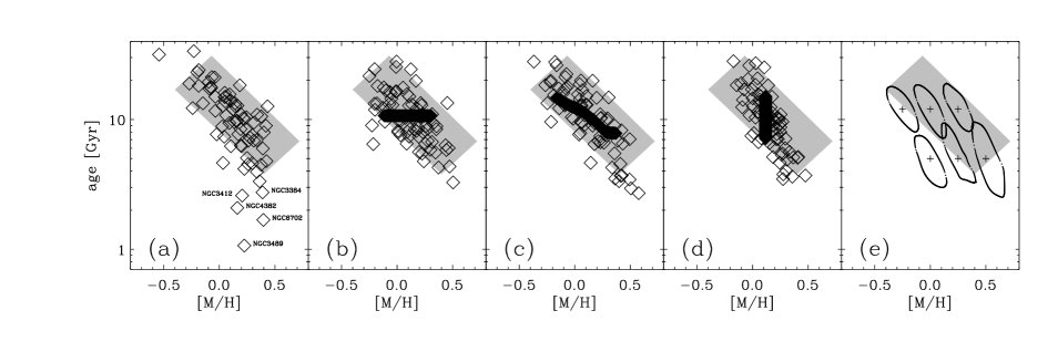
Figure 9: Age vs metallicity distributions: (a) our sample of 72 galaxies as derived from Figure 8a, (b) a Monte Carlo simulation with constant age and varying metallicity. The filled diamonds represent the input data set for the simulations, (c) a Monte Carlo simulation with varying age and varying metallicity, (d) a Monte Carlo simulations with constant metallicity, (e) error contours for selected points in the age-metallicity plane based on our median observational errors. The shaded area is the same in all diagrams and can be used to compare the distributions.

We can learn more from the MC simulations when we actually measure the ages and metallicities from the diagrams in Figure 8. This was done by interpolating between the model grid points and also linearly extrapolating if data points are outside the model predictions.

In the age/metallicity plane (Figure 9a) our observed sample follows a trend, such that more metal rich galaxies are also younger. This trend has recently been discussed by several authors (e.g., Jørgensen 1999, Trager et al. 2000b, Terlevich & Forbes 2000). However, analysing the MC simulation in Figure 9b we find that even a metallicity sequence at constant age is transformed into an age-metallicity correlation due to correlated errors in age/metallicity diagnostic diagrams such as Figure 8. For comparison we show in Figure 9c a MC simulation with both, age and metallicity variations and in Figure 9d a MC simulation with constant metallicity as input. The correlated errors stem from the fact that an error in e.g., the metallicity index results an error in both, the age and metallicity estimate, such that if the age is underestimated the galaxy seems also more metal rich and vice versa. Error contours in the age/metallicity plane, based on our median observational errors, for selected ages and metallicities are shown in Figure 9e. The contours are elongated mainly in the direction of a negative correlation of age and metallicity, however the detailed shape depends on the exact position within the age/metallicity plane. We note, that the error contours in Figure 9e reflect only the observational errors in our index measurements and do not include any errors in our determination of [Mg/Fe]. As demonstrated in section 4.2 they do also lead to an artificial age/metallicity correlation.

The effects of correlated errors will be present in diagrams such as Figure 8 as long as the index-combination does not completely resolve the age/metallicity degeneracy. Therefore any findings based on these diagrams such as age-metallicity correlations depend crucially on the size of the errors in the observables. Ideally one would prefer errors in ${\mathrm{H}}\beta$ $<0.1$ Å, however, large samples such as the Coma compilation by Jørgensen (1999) and the Lick extragalactic database [Trager et al. 1998] show typical errors of 0.2 to 0.3 Å with a tail of even larger errors making a proper age/metallicity analysis impossible. Our sample has a median error of 0.17 Å in ${\mathrm{H}}\beta$ with the largest being 0.23 Å and therefore is perhaps just at the borderline where one can start a useful age/metallicity analysis.

We note, that our sample contains a small number of galaxies with young stellar populations which tend to be more metal rich than the average galaxy. Looking back at the Mg–$\sigma$ relation shown in Figure 4a only NGC 3489 and NGC 4382 do clearly deviate towards lower Mg b ^′ values, the other galaxies with young stellar populations are consistent with the main relation which in turn can be perhaps best explained by a negative correlation of age and metallicity which holds these galaxies on the main relation (see also Figure 12).

For the remaining galaxies in our sample we do not find clear evidence of an age-metallicity anti-correlation and therefore conclude that the scatter at a given $\sigma$ in the Mg b ^′–$\sigma$ relation is not significantly reduced due to an age-metallicity ‘conspiracy’.

6 Corrected index–$\sigma$ relations

Of course the correction of the Mg b and $<$Fe$>$ indices for NSAR will also affect the index–$\sigma$ relations. The corrected versions are shown in Figure 10. Here we find ‘corrected’ fits (fitexy routine) of

$${\mathrm{M}g{\,\it b}}\,^{\prime}_{\mathrm{c}orr}=0.091(\pm 0.010)\log\sigma-0.068(\pm 0.023)\,,$$ (6)

and

$$<{\mathrm{F}e\,^{\prime}}>_{\mathrm{c}orr}=0.044(\pm 0.006)\log\sigma-0.012(\pm 0.014)\,.$$ (7)

Figure 10: (a) The Mg b ^′–$\sigma$, (b) $<\mathrm{Fe}\,^{\prime}\negthinspace>$–$\sigma$ and (c) ${\mathrm{H}}\beta\,^{\prime}$–$\sigma$ relations corrected for non-solar abundance ratios. The solid lines indicate a straight line fit taking into account error in both variables. The plus signs in panel (c) indicate galaxies which were excluded from the fit via an iterative scheme, see text for details. Error bars representing the median errors in each quantity are shown in the upper right corner of each panel.

The scatter about the Mg b ^′_corr–$\sigma$ relation is reduced to 0.010. However, the corrections of the Mg b index for NSAR are based on the Mg b vs $<$Fe$>$ diagram thus correlated errors are again present and we cannot draw any firm conclusions about the reduced scatter when we take the size of our observational errors into account.

Compared with the un-corrected versions, the Mg b ^′_corr–$\sigma$ relation shows a shallower slope whereas the $<\mathrm{Fe}\,^{\prime}\negthinspace>$_corr–$\sigma$ relation is steeper. This may seem to be an obvious result of the NSAR corrections, nevertheless it is important as the following shows. Using the W94 models and assuming that there are no age variations along the metal index–$\sigma$ relations, one can translate the slopes into changes of [M/H], giving $\Delta{\mathrm{[}M/H]}/\Delta\log\sigma=1.00\pm 0.11$ dex and $=0.83\pm 0.11$ dex for Mg b ^′ and $<\mathrm{Fe}\,^{\prime}\negthinspace>$ respectively (see also Table 3). This shows that the corrected index–$\sigma$ relations give now consistent measurements of the (total) metallicity change with central velocity dispersion, i.e., there is no need to invoke an additional age trend along the sequence after the correction for NSAR. We conclude that the disagreement in the strength of the metallicity change with $\log\sigma$, as estimated from the $<\mathrm{Fe}\,^{\prime}\negthinspace>$– and Mg b ^′–$\sigma$ relations, can be resolved if NSAR are taken into account.

As a consistency test, we show in Figure 10c the ${\mathrm{H}}\beta\,^{\prime}$_corr–$\sigma$ relation. If there is no age trend along the index–$\sigma$ relations, then the slope of our most age-sensitive index should only reflect the change in metallicity along the sequence. Towards the low $\sigma$ range we can see the galaxies with strong ${\mathrm{H}}\beta$ absorption deviating from the main ${\mathrm{H}}\beta$–$\sigma$ relation. Due to these strong deviations it is difficult to establish a fit which represents the overall slope. We therefore used an iterative scheme where we excluded all galaxies deviating by more than 3$\sigma$ from the fit (2 iterations, indicated in Figure 10c by plus signs). The best fitting relation is:

$${\mathrm{H}}\beta\,^{\prime}_{\mathrm{c}orr}=-0.031(\pm 0.008)\log\sigma+0.133(\pm 0.019)\,.$$ (8)

Using the W94 stellar population models and assuming no age trend along the sequence the fit translates into $\Delta{\mathrm{[}M/H]}/\Delta\log\sigma=1.00\pm 0.26$ dex, which is in good agreement with the above results.

If we assume an age-metallicity anti-correlation such as the one shown in Figure 8d ($7.8\leq age\leq 14.6$, $-0.17\leq{\mathrm{[}M/H]}\leq 0.37$) the models predict a slope in the ${\mathrm{H}}\beta$–$\sigma$ relation of –0.005, which is close to no change in ${\mathrm{H}}\beta$ with central velocity dispersion. This is inconsistent with our data on the $3-4\sigma$ level. Taking the 1$\sigma$ error of the observed ${\mathrm{H}}\beta$–$\sigma$ slope into account, allows only for an age gradient of 2 to 3 Gyrs along the sequence.

We conclude that the slope of the ${\mathrm{H}}\beta\,^{\prime}$_corr–$\sigma$ relation is consistent with the other index–$\sigma$ relations and our assumption of no age trend along the index–$\sigma$ relations within the fitting errors. Although there are some individual galaxies which show signs of an age-metallicity anti-correlation which can reduce the spread of scaling relations at a given mass, we do not favour a picture where such a correlation acts along the scaling relations.

We emphasize that although the total metallicity increases by $0.9\pm 0.1$ dex per dex in $\sigma$, individual elements can contribute differently to the increase. For example Fe seems to change only very little whereas magnesium (and probably other $\alpha$-elements) show a steeper increase.

In agreement with previous investigations into the [Mg/Fe] ratios [Worthey, Faber & González 1992, Jørgensen 1999, Kuntschner 2000, Trager et al. 2000b] we find that the [Mg/Fe] ratio slowly increases with the central velocity dispersion (or luminosity). Using the method of Trager et al. to measure the NSAR we estimate $0.05\leq\mathrm{[Mg/Fe]}\leq 0.30$ in the range $100\leq\sigma\leq 400$ (Figure 11). The largest [Mg/Fe] ratios are approximately 0.1 dex lower than what was estimated with previous methods [Worthey, Faber & González 1992, Weiss, Peletier & Matteucci 1995, Jørgensen 1999, Kuntschner 2000]. We note, that towards the low velocity dispersion range of our data, early-type galaxies still show non-solar abundance ratios suggesting that early-type galaxies with solar abundance ratios, if they exist at all, have velocity dispersions below $\sim$100 km s^-1.

We further note, that there are low luminosity galaxies exhibiting [Mg/Fe] ratios similar to much more luminous galaxies. The best confirmed case here is NGC 4464 [Peletier 1999, Vazdekis et al. 2000]. This in turn suggests that the [Mg/Fe]–$\sigma$ relation may show a significant scatter which would be responsible for some of the scatter in the Mg–$\sigma$ relation. The best fitting [Mg/Fe]–$\sigma$ relation is

$${\mathrm{[}Mg/Fe]}=0.30(\pm 0.06)\log\sigma-0.52(\pm 0.15)\,.$$ (9)

A (non-parametric) Spearman rank-order test shows a correlation coefficient of 0.40 with a significance level of $<0.1$%. The rather small correlation coefficient indicates that this relation shows a lot of scatter. However, it is again very sensitive to selection effects at the low $\sigma$ end which is not well represented in our data set. The relation found for our sample is in excellent agreement with the results of Trager et al. (2000b; Fig. 11, dashed line). We note, that Jørgensen’s (1999) analysis of Coma galaxies indicates a much steeper slope of $\Delta{\mathrm{[}Mg/Fe]}/\Delta\log\sigma\simeq 1.1$.

Figure 11: [Mg/Fe] vs $\log\sigma$ relation. The median observational errors are indicated in the right upper corner. The solid line shows a straight line fit taking into account errors in both variables. The dashed line represents the best fitting relation to the sample of Trager et al. (2000b).

Finally we want to present the correlations between our derived ages and metallicities with the central velocity dispersion. We note, that the derived parameters carry all the caveats mentioned in the previous sections. Figure 12a and b show the [M/H]– & $\log$ age–$\sigma$ relations respectively. Although there is substantial spread in the relations it can be clearly seen that our derived metallicities are consistent with an increase of $\Delta{\mathrm{[}M/H]}/\Delta\log\sigma\simeq 0.9$ (indicated by the dashed line in Figure 12a). A (non parametric) Spearman rank-order test shows a weak correlation coefficient of 0.33 with a significance level of $0.4$%. The change in metallicity per dex in $\log\sigma$ is in good agreement with the relation found by Kuntschner (2000) for the Fornax cluster and by Trager et al. (2000b) for early-type galaxies in groups and clusters. Our best age estimates do not show a significant correlation with $\sigma$ (Spearman rank-order test: correlation coefficient $=0.10$, significance level $=40$%). However, we emphasize that the age spread increases towards the low $\sigma$ end of the relation. For a similar result see Concannon, Rose & Caldwell (2000).

Figure 12: (a) The [M/H]–$\sigma$ relation and, (b) the $\log$ age–$\sigma$ relation for our sample of 72 galaxies. The ages and metallicities are derived from Figure 8a. The dashed line in panel (a) is not a fit to the data but represents a slope of 0.9 dex in metallicity per dex in $\log\sigma$.

7 CONCLUSIONS

For our sample of 72 early-type galaxies, drawn mostly from clusters and groups, we have analysed the Mg b ^′–$\sigma$ and $<\mathrm{Fe}\,^{\prime}\negthinspace>$–$\sigma$ relations as well as age/metallicity diagnostic diagrams with up-to-date stellar population models. Taking the effects of non-solar abundance ratios into account, we conclude:

• Tight index-$\sigma$ relations, as well as the results from age/metallicity diagnostic diagrams, provide evidence that cluster early-type galaxies are made of old stellar populations (age $>$7 Gyrs) and follow mainly a trend of increasing metallicity with increasing central velocity dispersion $\sigma$. The galaxies display no or at most a mild age-trend along the sequence. A small number ($\sim$5) of galaxies show younger luminosity weighted ages and above average metallicities in their mean stellar populations. These galaxies have velocity dispersions below $\sim$170 km s^-1.

• Correcting the line-strength indices for non-solar abundance ratios is a crucial step forward in deriving more reliable age-metallicity estimates. Correlated errors, however, in age/metallicity diagnostic diagrams combined with the precision of currently available index measurements for medium to large samples lead to artificial anti-correlations between age and metallicity estimates. Therefore it is difficult to differentiate between mild anti-correlations between age and metallicity and a pure metallicity sequence. For the majority of our sample we do not find evidence for a prominent age/metallicity correlation and we can firmly exclude a pure age sequence at constant metallicity.

• Correcting the Mg b and $<$Fe$>$ indices for non-solar abundance ratios changes the slope of the index–$\sigma$ relations in the sense that the Mg–$\sigma$ relation becomes shallower and the $<$Fe$>$–$\sigma$ relation becomes steeper. The ${\mathrm{H}}\beta$–$\sigma$ relation remains virtually unchanged. Under the assumption of no age gradients along the index–$\sigma$ relations all three index–$\sigma$ relations give consistent estimates of the total metallicity change per dex in $\log\sigma$: $\Delta{\mathrm{[}M/H]}/\Delta\log\sigma=1.00\pm 0.11$, $0.83\pm 0.11$ and $1.00\pm 0.26$ for the Mg b–$\sigma$, $<$Fe$>$–$\sigma$, and ${\mathrm{H}}\beta$–$\sigma$ relations respectively. Introducing an age gradient along the sequence leads readily to inconsistent results of model predictions and the slope of the ${\mathrm{H}}\beta$–$\sigma$ relation. At most an age gradient of 2 to 3 Gyr along the scaling relations is within our measurement errors.

• The [Mg/Fe] ratio is mildly correlated with the central velocity dispersion and ranges from ${\mathrm{[}Mg/Fe]}=0.05$ to 0.3 for galaxies with $\sigma\geq 100$ km s^-1. Some low luminosity galaxies, such as NGC 4464, do not follow the main trend but show [Mg/Fe] ratios similar to the more luminous galaxies.

Appendix A Line strength indices

Table 5 lists the name, environment, central velocity dispersion and line-strength indices for all 72 galaxies in our sample.

Table 5: Index Measurements

Name	env.	S/N	$\log\sigma_{0}$	$\epsilon_{\sigma_{0}}$	${\mathrm{H}}\beta$	$\epsilon_{\mathrm{H}\beta}$	Mg2	$\epsilon_{\mathrm{Mg}_{2}}$	Mg b	$\epsilon_{\mathrm{Mg}\/b}$	$<$Fe$>$	$\epsilon_{<\mathrm{Fe}>}$	[OIII]$\lambda 5007$
NGC 2300	A569	45	2.427	0.014	1.53	0.15	0.311	0.005	4.92	0.16	2.88	0.14	-
NGC 2320	A569	36	2.508	0.022	1.67	0.21	0.295	0.006	5.18	0.20	2.96	0.18	-1.98
NGC 2329	A569	32	2.359	0.024	1.30	0.23	0.270	0.006	4.13	0.23	2.79	0.20	-0.37
NGC 2340	A569	34	2.386	0.016	1.33	0.21	0.340	0.006	5.25	0.21	3.51	0.18	-
NGC 2513	-	47	2.420	0.014	1.60	0.15	0.329	0.004	4.88	0.16	2.93	0.14	-
NGC 2634	Group	40	2.276	0.014	1.50	0.18	0.286	0.005	4.45	0.18	2.65	0.16	-0.37
NGC 2672	Group	34	2.423	0.023	1.88	0.19	0.337	0.006	5.21	0.21	2.55	0.19	-
NGC 2693	Group	32	2.541	0.022	1.21	0.21	0.320	0.007	5.34	0.23	3.11	0.20	-
NGC 2768	Group	36	2.251	0.014	1.82	0.21	0.285	0.006	4.65	0.20	2.84	0.18	-1.16
NGC 2778	Group	50	2.192	0.012	1.55	0.15	0.294	0.004	4.44	0.15	2.92	0.13	-0.65
NGC 3377	Leo I	55	2.190	0.011	1.84	0.13	0.234	0.004	4.01	0.13	2.63	0.12	-0.27
NGC 3379	Leo I	59	2.323	0.010	1.46	0.12	0.287	0.004	4.75	0.12	2.76	0.11	-0.34
NGC 3384	Leo I	59	2.174	0.008	2.05	0.11	0.265	0.003	3.96	0.12	2.95	0.11	-
NGC 3412	Leo I	52	2.005	0.012	2.23	0.14	0.201	0.004	3.43	0.14	2.74	0.13	-
NGC 3489	Leo I	67	2.005	0.011	3.63	0.11	0.151	0.003	2.51	0.11	2.40	0.10	-1.62
NGC 3608	Group	57	2.264	0.011	1.59	0.13	0.288	0.004	4.43	0.13	2.76	0.12	-0.28
NGC 4365	Virgo	49	2.387	0.012	1.72	0.14	0.303	0.004	4.96	0.15	3.11	0.13	-
NGC 4374	Virgo	58	2.443	0.011	1.43	0.13	0.295	0.004	4.79	0.13	2.54	0.11	-0.86
NGC 4382	Virgo	48	2.234	0.012	2.49	0.14	0.227	0.004	3.32	0.15	2.59	0.14	-
NGC 4406	Virgo	48	2.373	0.010	1.61	0.16	0.286	0.005	4.65	0.16	2.82	0.15	-
NGC 4434	Virgo	36	2.080	0.016	1.77	0.19	0.250	0.006	3.90	0.20	2.30	0.18	-
NGC 4458	Virgo	32	2.004	0.024	2.15	0.22	0.245	0.006	3.76	0.23	2.43	0.20	-0.28
NGC 4464	Virgo	39	2.162	0.014	1.92	0.18	0.235	0.005	4.06	0.19	2.37	0.17	-
NGC 4472	Virgo	55	2.477	0.012	1.42	0.13	0.340	0.004	5.03	0.13	3.37	0.12	-
NGC 4473	Virgo	78	2.264	0.007	1.42	0.09	0.300	0.003	4.62	0.09	3.10	0.08	-
NGC 4552	Virgo	60	2.384	0.011	1.40	0.13	0.308	0.004	4.86	0.13	2.93	0.11	-0.22
NGC 4564	Virgo	46	2.170	0.013	1.78	0.15	0.312	0.005	4.79	0.16	3.00	0.14	-
NGC 4621	Virgo	68	2.379	0.010	1.43	0.11	0.360	0.003	5.21	0.11	3.17	0.10	-
NGC 4649	Virgo	47	2.524	0.013	1.61	0.16	0.325	0.005	5.00	0.16	2.81	0.14	-0.23
NGC 4660	Virgo	64	2.290	0.009	1.35	0.11	0.319	0.003	4.72	0.11	2.70	0.10	-
NGC 4673	Coma	43	2.356	0.013	1.93	0.16	0.269	0.004	4.14	0.16	2.81	0.15	-0.46
NGC 4692	Coma	30	2.389	0.019	1.51	0.22	0.308	0.007	4.65	0.24	3.07	0.20	-
NGC 4789	Coma	45	2.421	0.014	1.54	0.15	0.299	0.004	4.46	0.16	2.84	0.14	-
NGC 4807	Coma	46	2.289	0.012	1.61	0.15	0.282	0.004	4.50	0.15	3.17	0.14	-
NGC 4827	Coma	31	2.390	0.019	1.49	0.21	0.310	0.007	4.84	0.23	2.80	0.20	-
NGC 4839	Coma	42	2.443	0.016	1.50	0.16	0.313	0.005	5.19	0.17	3.01	0.15	-
NGC 4840	Coma	32	2.363	0.020	1.66	0.22	0.313	0.006	5.07	0.22	2.61	0.20	-
NGC 4841A	Coma	47	2.389	0.014	1.33	0.15	0.303	0.004	4.77	0.15	2.74	0.13	-0.20
NGC 4841B	Coma	40	2.232	0.014	1.81	0.18	0.277	0.005	4.33	0.18	2.91	0.16	-0.44
NGC 4860	Coma	41	2.436	0.014	1.53	0.16	0.330	0.005	4.98	0.17	2.81	0.15	-
NGC 4864	Coma	43	2.309	0.014	1.85	0.17	0.278	0.005	4.51	0.17	2.79	0.15	-0.43
NGC 4869	Coma	31	2.306	0.019	1.01	0.22	0.304	0.007	4.78	0.23	2.63	0.20	-
NGC 4874	Coma	35	2.453	0.019	1.80	0.21	0.306	0.006	4.62	0.21	2.66	0.19	-0.28
NGC 4876	Coma	37	2.276	0.016	1.44	0.18	0.239	0.005	3.95	0.19	2.98	0.17	-
NGC 4881	Coma	37	2.293	0.018	1.62	0.19	0.293	0.005	4.83	0.19	3.06	0.17	-
NGC 4886	Coma	31	2.227	0.019	1.78	0.21	0.248	0.006	4.32	0.23	2.83	0.20	-
NGC 4889	Coma	44	2.601	0.017	1.51	0.16	0.334	0.005	5.56	0.17	3.00	0.15	-
NGC 4908	Coma	33	2.293	0.019	1.69	0.21	0.289	0.006	4.28	0.21	2.80	0.18	-0.34
NGC 4926	Coma	44	2.432	0.014	1.56	0.16	0.315	0.005	5.23	0.16	3.06	0.14	-
NGC 4952	Coma	45	2.453	0.014	1.61	0.15	0.266	0.005	4.41	0.16	2.93	0.14	-
NGC 5582	-	35	2.095	0.019	1.69	0.19	0.253	0.006	4.12	0.21	2.46	0.19	-
NGC 5638	Group	48	2.231	0.013	1.48	0.17	0.321	0.005	5.17	0.18	2.89	0.16	-
NGC 5812	-	61	2.280	0.010	1.65	0.13	0.298	0.004	4.51	0.14	2.99	0.12	-
NGC 5813	Group	56	2.377	0.012	1.64	0.15	0.285	0.004	4.45	0.15	2.85	0.13	-0.41
NGC 5831	Group	53	2.200	0.012	1.47	0.15	0.269	0.005	4.32	0.16	2.78	0.14	-
NGC 5846	Group	48	2.344	0.013	1.52	0.18	0.307	0.005	5.05	0.18	2.55	0.16	-0.50
NGC 5982	Group	34	2.362	0.020	1.86	0.21	0.269	0.006	4.08	0.22	2.70	0.19	-
NGC 6127	-	53	2.373	0.013	1.62	0.14	0.286	0.004	4.65	0.15	2.98	0.13	-0.22
NGC 6702	-	37	2.196	0.020	2.47	0.22	0.214	0.006	3.78	0.22	2.70	0.19	-0.30
NGC 6703	-	56	2.265	0.013	2.00	0.14	0.280	0.004	4.22	0.15	2.79	0.13	-0.54
continued on next page

Table 6: continued

Name	env.	S/N	$\log\sigma_{0}$	$\epsilon_{\sigma_{0}}$	${\mathrm{H}}\beta$	$\epsilon_{\mathrm{H}\beta}$	Mg2	$\epsilon_{\mathrm{Mg}_{2}}$	Mg b	$\epsilon_{\mathrm{Mg}\/b}$	$<$Fe$>$	$\epsilon_{<\mathrm{Fe}>}$	[OIII]$\lambda 5007$
IC 0613	A1016	32	2.434	0.021	1.69	0.20	0.322	0.006	5.21	0.21	2.26	0.19	-
IC 3973	Coma	38	2.341	0.016	1.78	0.17	0.283	0.005	4.46	0.19	2.51	0.17	-
IC 4011	Coma	30	1.982	0.029	1.51	0.22	0.260	0.007	4.19	0.24	2.55	0.21	-
IC 4045	Coma	35	2.327	0.016	1.36	0.20	0.283	0.006	4.54	0.20	2.50	0.18	-
D024	Coma	35	2.279	0.015	1.54	0.21	0.287	0.006	4.38	0.21	2.70	0.19	-
D081	Coma	30	2.067	0.021	1.54	0.22	0.247	0.007	4.15	0.24	2.36	0.22	-
D210	Coma	35	2.148	0.022	1.27	0.20	0.239	0.006	3.87	0.21	2.09	0.19	-
GMP 1652	Coma	35	2.143	0.018	1.71	0.19	0.270	0.006	4.25	0.20	2.88	0.18	-
Z159-43	Coma	31	2.415	0.021	1.50	0.23	0.315	0.007	4.84	0.23	2.86	0.20	-0.78
Z160-22	Coma	30	2.377	0.020	1.49	0.23	0.312	0.007	4.83	0.23	2.72	0.21	-
Z160-23	Coma	30	2.218	0.018	1.45	0.23	0.283	0.007	4.73	0.24	2.98	0.21	-
Z160-27	Coma	30	2.135	0.017	1.67	0.23	0.278	0.007	4.14	0.24	2.63	0.21	-0.30

Notes: The first column shows the name of the galaxy. If the galaxy is found in the NGC or IC (Nilson 1973) catalogues, then it will have the name from the corresponding catalogue, in the order of preference given above. There are also some galaxies denoted by their name from the CGCG (Zwicky et al. 1961, Zxxx-xx) catalogue, Dressler’s (1980, Dxxx) catalogue and one galaxy found in the Godwin, Metcalfe & Peach catalogue (1983, GMP 1652). The second column indicates the environment. If the galaxy is a member of a well known cluster or group, the name is given. For smaller associations we just indicate whether the galaxies are in a very low density environment (“-”) or belong to a group. The third column shows the effective S/N per Å of the line-strength measurements. The velocity dispersion $\sigma_{0}$ and the line-strength indices have been aperture corrected to $2r_{norm}=1.19h^{-1}\,$kpc, equivalent to 3$\aas@@fstack{\prime\prime}$4 at the distance of the Coma cluster. The line-strength indices are calibrated onto the Lick/IDS system and corrected to zero velocity dispersion with the exception of the [OIII]$\lambda 5007$ index which is calibrated to the González (1993) system. Mg₂ is given in mag, whereas the other line-strength indices are given in Å.

References

- [Bender, Burstein & Faber 1993] Bender R., Burstein D., Faber S. M., 1993, ApJ, 411, 153
- [Bower, Lucey & Ellis 1992] Bower R. G., Lucey J. R., Ellis R. S., 1992, MNRAS, 254, 601
- [Burstein et al. 1988] Burstein D., Davies R. L., Dressler A., Faber S. M., Lynden-Bell D., Terlevich R. J., Wegner G., 1988, in Kron R. G. and Renzini A., eds, Towards Understanding Galaxies at Large Redshifts, page 17, Dordrecht, Kluwer
- [Butcher & Oemler 1978] Butcher H., Oemler A., 1978, ApJ, 219, 18
- [Butcher & Oemler 1984] Butcher H., Oemler A., 1984, ApJ, 285, 426
- [Cole et al. 2000] Cole, S., Lacey, C. G., Baugh, C. M., Frenk, C. S. 2000, MNRAS, 319, 168
- [Colless et al. 1999] Colless M., Burstein D., Davies R. L., McMahan R. K., Saglia R. P., Wegner G., 1999, MNRAS, 303, 813
- [Concannon, Rose & Caldwell 2000] Concannon K. D., Rose J. A., Caldwell N., 2000, ApJL, 536, L19
- [Couch et al. 1998] Couch W. J., Barger A. J., Smail I., Ellis R. S., Sharples R. M., 1998, ApJ, 497, 188
- [Davies, et al. 1987] Davies R. L., Burstein D., Dressler A., Faber S. M., Lynden-Bell D., Terlevich R. J., Wegner G., 1987, ApJS, 64, 581
- [de Jong & Davies 1997] de Jong R. S., Davies R. L., 1997, MNRAS, 285, L1
- [Djorgovski & Davis 1987] Djorgovski S., Davis M, 1987, ApJ, 313, 59
- [Dressler 1980] Dressler A., 1980, ApJS, 42, 565
- [Dressler 1984] Dressler A., 1984, ApJ, 281, 512
- [Dressler et al. 1987] Dressler A., Lynden-Bell D., Burstein D., Davies R. L., Faber S. M., Terlevich R. J., Wegner G., 1987, ApJ, 313, 42
- [Dressler, et al. 1997] Dressler A. et al., 1997, ApJ, 490, 577
- [Ellis et al. 1997] Ellis R. S., Smail I., Dressler A., Couch W. J., Oemler A. J., Butcher H., Sharples R. M., 1997, ApJ, 483, 582
- [Ferreras, Charlot & Silk 1999] Ferreras I., Charlot S., Silk J. 1999, ApJ, 521, 81
- [Fisher, Franx & Illingworth 1996] Fisher D., Franx M., Illingworth G., 1996, ApJ, 459, 110
- [González 1993] González J. J., 1993, PhD thesis, University of California
- [Godwin, Metcalfe & Peach1983] Godwin, J. G., Metcalfe, N., Peach, J. V., 1983, MNRAS, 202, 113
- [Gorgas, Efstathiou & Aragon-Salamanca 1990] Gorgas J., Efstathiou G., Salamanca A. A., 1990, MNRAS, 245, 217
- [Greggio 1997] Greggio L., 1997, MNRAS, 285, 151
- [Hudson et al. 1999] Hudson M.J., Smith R.J., Lucey J.R., Schlegel D.J., Davies R.L., 1999, ApJ, 512, L79
- [Jørgensen, Franx & Kjærgaard 1995] Jørgensen I., Franx M., Kjærgaard P., 1995, MNRAS, 276, 1341
- [Jørgensen 1997] Jørgensen I., 1997, MNRAS, 288, 161
- [Jørgensen 1999] Jørgensen I., 1999, MNRAS, 306, 607
- [Kodama et al. 1998] Kodama T., Arimoto N., Barger A. J., Arag’on-Salamanca A., 1998, A&A, 334, 99
- [Kuntschner 1998] Kuntschner H., 1998, PhD thesis, University of Durham
- [Kuntschner & Davies 1998] Kuntschner H., Davies R. L., 1998, MNRAS, 295, L29
- [Kuntschner 2000] Kuntschner H., 2000, MNRAS, 315, 184
- [Larson, Tinsley & Caldwell 1980] Larson R. B., Tinsley B. M., Caldwell C. N., 1980, ApJ, 237, 692
- [Longhetti et al. 1998] Longhetti M., Rampazzo R., Bressan A., Chiosi C., 1998, A&AS, 130, 251
- [Mehlert 1998] Mehlert D., 1998, PhD thesis, Ludwig - Maximilian - Universiät, München
- [Mehlert et al. 2000] Mehlert D., Saglia R. P., Bender R., Wegner G., 2000, A&AS, 141, 449
- [Nilson 1973] Nilson P., 1973, Uppsala General Catalogue of Galaxies, Uppsala Astron. Obs. Ann., 6 (UGC)
- [O’Connell 1976] O’Connell R. W., 1976, ApJ, 206, 370
- [Peletier 1989] Peletier R. F., 1989, PhD thesis, University of Groningen
- [Peletier 1999] Peletier R. F., 1999, in Beckman J. E. and Mahoney T. J., eds, ASP Conf. Ser. Vol 187, The Evolution of Galaxies on Cosmological Timescales. Astron. Soc. Pac., San Francisco, p. 231
- [Press et al. 1992] Press W. H., Teukolsky S. A., Vetterling W. T., Flannery B. P., 1992, Numerical Recipes – Second Edition, Cambridge University Press, UK
- [Renzini & Ciotti 1993] Renzini A., Ciotti L., 1993, ApJL, 416, L49
- [Salaris & Weiss 1998] Salaris M., Weiss A., 1998, A&A, 335, 943
- [Sandage & Visvanathan 1978] Sandage A., Visvanathan N., 1978, ApJ, 223, 707
- [Smith et al. 2000] Smith R.J., Lucey J.R., Hudson M.J., Schlegel D.J., Davies R.L., 2000, MNRAS, 313, 469
- [Tantalo, Chiosi & Bressan 1998] Tantalo R., Chiosi C., Bressan A., 1998, A&A, 333, 419
- [Terlevich et al. 1981] Terlevich R., Davies R. L., Faber S. M., Burstein D., 1981, MNRAS, 196, 381
- [Terlevich & Forbes 2000] Terlevich A., Forbes D. A., submitted to MNRAS
- [Trager 1997] Trager, S. C., 1997, PhD thesis, University of California, CA
- [Trager et al. 1998] Trager S. C., Worthey G., Faber S. M., Burstein D., Gonzalez J. J., 1998, ApJS, 116, 1
- [Trager et al. 2000a] Trager S. C., Faber S. M., Worthey G., González J. J., 2000a, AJ, 119, 1645
- [Trager et al. 2000b] Trager S. C., Faber S. M., Worthey G., González J. J., 2000b, AJ, 120, 165
- [Tripicco & Bell 1995] Tripicco M. J., Bell R. A., 1995, AJ, 110, 3035
- [Vazdekis et al. 2000] Vazdekis A., Kuntschner H., Davies R. L., Arimoto N., Nakamura O., Peletier R. F., 2000, submitted to ApJL
- [van Dokkum et al. 1998] van Dokkum P. G., Franx M., Kelson D. D., Illingworth G. D., Fisher D., Fabricant D., 1998, ApJ, 500, 714
- [Weiss, Peletier & Matteucci 1995] Weiss A., Peletier R. F., Matteucci F., 1995, A&A, 296, 73
- [Worthey 1998] Worthey G., 1998, PASP, 110, 888
- [Wegner et al. 1999] Wegner G., Colless M., Saglia R. P., McMahan R. K., Davies R. L., Burstein D., Baggley G., 1999, MNRAS, 305, 259
- [Worthey, Faber & González 1992] Worthey G., Faber S. M., González J. J., 1992, ApJ, 398, 69
- [Worthey 1994] Worthey G., 1994, ApJS, 95, 107 (W94)
- [Worthey & Ottaviani 1997] Worthey G., Ottaviani D. L., 1997, ApJS, 111, 377
- [Zwicky et al. 1961] Zwicky F., Herzog W., Wild P., Karpowicz M., Kowal C., 1961-68, Catalogue of Galaxies and Clusters of Galaxies. California institute of Technology, Pasadena (CGCG)