Abstract

Chiral cosmic strings are naturally produced at the end of D-term inflation and they may have interesting cosmological consequences. As was first proved by Carter and Peter, the equations of motion for chiral cosmic strings in Minkowski space are integrable (just as for Nambu-Goto strings). Their solutions are labeled by a function $k(\sigma-t)$ where $t$ is time and $\sigma$ is the invariant length along the string, and the constraints on $k$, which determines the charge on the string, are that $0\leq k^{2}\leq 1$. We review the origin of this parameter and also discuss some general properties of such strings which can be deduced from the equations of motion. The metric around infinite chiral strings is then constructed in the weak field limit, and studied as a function of $k$. We also consider the angular momentum of circular chiral loops, and extend previous work to consider the evolution and self-intersection properties of a more general family of chiral cosmic string loops for which $k^{2}(\sigma-t)$ is not constant.

1 Introduction

In the last few years the scenario of structure formation from cosmic strings has become increasingly tenuous, since its predictions differ significantly from the new high accuracy measurements of the temperature fluctuations in the cosmic microwave background radiation. Most studies of such observational consequences of strings have focused on structureless Nambu-Goto (NG) strings [1, 2, 3, 4, 5] and global strings [6, 7], and in each case the recent predictions are based on numerical simulations of the evolution of the string network postulated to form at the GUT phase transition. One should recall though that there are some unresolved and potentially important uncertainties in the simulations — it is very difficult, for example, to resolve the very disparate scales which characterize the the network, as well as to deal with gravitational backreaction effect — and hence a combination of numerical work with analytical modeling [1, 4, 5] has also been used to make predictions from NG strings.

Our focus here is not on NG strings but rather on chiral cosmic strings. These strings are a type of current carrying string [8] for which the world-sheet current $j^{i}$ is null;

$$j^{i}j_{i}=j^{2}=0.$$

(Here $i=(0,1)$ and the 2D world sheet metric $\gamma_{ij}$ defined below raises and lowers indices.) One motivation for studying such chiral strings comes from the well known SUSY D-term inflation model. In this model, strings are produced at the end of inflation [9] so that both mechanisms contribute to producing density fluctuations. However, the strings produced are chiral cosmic strings and not NG strings [10]. Hence in order to make predictions for the $C_{l}$’s from this ‘strings plus inflation’ model, the evolution and cosmological consequences of chiral cosmic string networks must be understood. (There may exist models in which the strings formed at the end of inflation are NG ones, however this is not true of D-term inflation. In the case of ‘inflation plus NG strings’, predictions may be found in [11].)

There are a number of differences between the properties of chiral cosmic strings and NG strings. One such regards the evolution of the strings themselves: the null current on chiral strings can, as in the case of other current-carrying strings, lead to the formation of non self-intersecting stable loops called vortons. This is potentially catastrophic as the energy density in the chiral string network could quickly dominate the energy density in the universe if stable vortons are present. It is therefore important to see if vortons are produced, and in section 4 we study the self-intersection properties of a family of chiral cosmic string loops. Another difference between NG and chiral strings is that these line-like sources of energy generate different metrics about them (section 3.2). One might therefore expect them to produce different perturbations in the matter and radiation through which they pass.

Recently a number of steps have been made which allow for a quantitative study of chiral cosmic string dynamics. First, a well defined unique 2D effective action exists for these strings [12, 15]. From this action it was shown, with suitable gauge choices, that the equations of motion are integrable in Minkowski space [15] (see also [16, 17] for different presentations of the same result). They are

$$\frac{\partial^{2}{\mathbf{x}}}{\partial t^{2}}-\frac{\partial^{2}{\mathbf{x}}}{\partial\sigma^{2}}=0\qquad\Longrightarrow\qquad{\mathbf{x}}(t,{\sigma})=\frac{1}{2}[{\mathbf{a}}(t+{\sigma})+{\mathbf{b}}(t-{\sigma})],$$ (1.1)

where $t$ is background time, and $\sigma$ measures the invariant length or energy along the string as in the NG case [16]. The constraints are

$$\mathaccent 19{{\mathbf{a}}}^{2}\!\!\! = \!\!\!1,$$ (1.2)

$$\mathaccent 19{{\mathbf{b}}}^{2}\!\!\! \leq \!\!\!1,$$ (1.3)

where for instance $\mathaccent 19{{\mathbf{a}}}(q)\equiv d{\mathbf{a}}(q)/dq.$ If one defines

$$k^{2}:=\mathaccent 19{{\mathbf{b}}}^{2}$$ (1.4)

so that $k=k(t-\sigma)$, then it can be shown that $k^{2}$ determines the conserved charge on the string (see also below). Furthermore, if $k=$ constant $=1$ then this charge vanishes as required, since $\mathaccent 19{{\mathbf{b}}}=1$ is just the Nambu-Goto limit. In reference [16], the self-intersection properties of chiral cosmic string loops were also studied in the special case of $k=$ constant. In particular the strings were shown never to self-intersect for $k=0$: this case corresponds to maximal charge on the strings and to vorton solutions.

Here that work is extended, though we still consider Minkowski space (with metric $\eta_{\mu\nu}=(+,-,-,-)$) throughout. First, for completeness, we indicate in section 2 how the equations of motion (1.1)-(1.3) are obtained from the chiral action and how the charge mentioned above is defined. This necessarily follows parts of reference [16] rather closely, though a small error in that paper is corrected. We also compare the chiral charge with the charges used for more general current carrying strings. In section 3 we summarize some properties of chiral cosmic strings which result from the equations of motion. The metric around infinite chiral strings is then studied as a function of $k$ and we comment in possible consequences it may have for structure formation and CMB anisotropies from chiral cosmic strings. In section 3.3, the effect of angular momentum on the motion of circular loops is considered by looking at the effective potential introduced in [18]. In section 4 we investigate the self-intersection properties of loops with non-constant $k$. Finally conclusions are given in section 5.

2 Review of chiral string equations of motion and charges

2.1 Action and charges

The effective 2D chiral string action has 2 terms: the first is the usual NG action, and the second results from the zero modes moving along the string. Let $\phi$ be a dimensionless real scalar field (the phase of the charge carriers) living on the 2D string world sheet labeled by coordinates $\sigma^{i}$. Then the action, which was first proposed by Carter and Peter [15], is

$$S=-\int d^{2}\sigma\,\sqrt{-\gamma}\left(m^{2}-\frac{1}{2}\psi^{2}\gamma^{ij}\phi_{,i}\phi_{,j}\right)$$ (2.1)

where $\gamma_{ij}=\eta_{\mu\nu}x^{\mu}_{,i}x^{\nu}_{,j}$ is the induced world sheet metric and $x^{\mu}(\sigma^{0},\sigma^{1})$ the position of the string. The dimensionless Lagrange multiplier $\psi^{2}$ sets the constraint

$$\gamma^{ij}\phi_{,i}\phi_{,j}=0\qquad\Longrightarrow\qquad\frac{1}{\sqrt{-\gamma}}\partial_{i}(\sqrt{-\gamma}\gamma^{ij}\phi_{,j})=0$$ (2.2)

so that $J^{i}=\gamma^{ij}\phi_{,j}$ is a conserved null current. The equation of motion $\delta S/\delta\phi=0$ defines another conserved null current $z^{i}$ by

$$\partial_{i}(\sqrt{-\gamma}\psi^{2}\gamma^{ij}\phi_{,j})=0\qquad\Longrightarrow\qquad z^{i}=\psi^{2}\gamma^{ij}\phi_{,j}.$$ (2.3)

As noted in [16], the action (2.1) in fact has an infinite number of null conserved currents $j^{i}=f(\phi)\phi^{,i}$ since equations (2.2) and (2.3) imply that $\psi=\psi(\phi)$. The degeneracy of currents is broken by observing that (2.1) is invariant not only under coordinate reparametrizations ${\sigma}^{i}\to\tilde{\sigma}^{i}=\tilde{\sigma}^{i}({\sigma}^{j})$ but also under transformations

$$\phi\to\tilde{\phi}(\phi),\qquad{\rm with}\qquad\psi\to\tilde{\psi}=\left({d\tilde{\phi}\over d\phi}\right)^{-1}\psi.$$ (2.4)

These freedoms are removed making gauge choices (see [15, 16] and below), so that the only definition of current which is invariant under (2.4) and hence independent of gauge choice is

$$j^{i}=\psi\phi^{,i}.$$ (2.5)

This is null and conserved and, from Green’s theorem, the corresponding conserved charge is

$$C=\int d\sigma^{i}\epsilon_{ik}j^{k},$$ (2.6)

where $\epsilon$ is the antisymmetric surface measure tensor whose square gives the induced metric; $\gamma_{ij}=\epsilon_{ik}\epsilon^{k}_{\;j}$ [15].

For current-carrying strings with time- or space-like currents, this degeneracy of possible conserved charges is broken. These strings are characterized by two independent conserved quantum numbers (see for example [18]). The first, $Z$, is defined through the Noether current $z^{i}$ given in (2.3): $Z=\int d\sigma^{i}\epsilon_{ik}z^{k}.$ The second, $N$ the integer winding number, is defined by the topological current $\tilde{j}^{i}=\frac{1}{2\pi}\epsilon^{ij}\phi_{,j}$ which is automatically conserved in 1+1D: $N=\int d\sigma^{i}\epsilon_{ik}\tilde{j}^{k}=\frac{1}{2\pi}\int d\phi$ ($\phi$ is defined modulo $2\pi$). As noted above, neither of these currents and corresponding charges are gauge invariant for chiral strings. The chiral charge $C$ is closely related to $N$ and $Z$ if one works in a gauge in which $\psi(\phi)$ is constant: on defining $\kappa_{0}=\psi^{2}$ then

$$C=\frac{Z}{\sqrt{\kappa_{0}}}=2\pi\sqrt{\kappa_{0}}N\qquad(\psi(\phi)\;=\;{\rm constant}).$$ (2.7)

This gauge was in particular chosen in reference [12]. As was discussed in detail in [15, 16], and as we now summarize briefly, the equations of motion resulting from (2.1) simplify greatly in a gauge for which $\psi(\phi)$ is not constant. (Indeed in this gauge, $\psi(\phi)$ is closely related to function $k$ mentioned in the introduction — see below.) Then there is no simple relation between $N$, $Z$ and $C$, and one must work with this latter gauge-independent charge.

2.2 Equations of motion

As was discussed in [15, 16], the equation of motion obtained by varying the action with respect to $x^{\mu}$;

$$\partial_{i}\left[\sqrt{-\gamma}\left(\gamma^{ij}+\frac{\psi^{2}}{m^{2}}\phi^{,i}\phi^{,j}\right)x^{\mu}_{,j}\right]=0,$$ (2.8)

simplifies greatly if reparametrization invariance is used to choose one of the coordinates to be $\eta=m^{-1}\phi$. It then follows from (2.2) that $\gamma^{\eta\eta}=0$ and, again as discussed in [15, 16], there is also freedom to choose $\psi^{2}=\gamma_{\eta\eta}=x_{,\eta}\cdot x_{,\eta}$. As a result equation (2.8) simplifies to

$$\partial_{q}\partial_{\eta}x^{\mu}=0,$$ (2.9)

where the second world-sheet coordinate has been denoted by $q$. Equation (2.9) still allows the coordinates $q$ and $\eta$ each to be transformed separately so that one can let

$$q=t+\sigma\qquad,\qquad\eta=t-\sigma$$

where $t=x^{0}$ is background time. In that case the wave equation (2.9) takes the familiar form given in (1.1):

$$\frac{\partial^{2}{\mathbf{x}}}{\partial t^{2}}-\frac{\partial^{2}{\mathbf{x}}}{\partial\sigma^{2}}=0\qquad\Longrightarrow\qquad{\mathbf{x}}(t,{\sigma})=\frac{1}{2}[{\mathbf{a}}(t+{\sigma})+{\mathbf{b}}(t-{\sigma})].$$

The constraints coming from $\gamma^{\eta\eta}=0$ and $\psi^{2}=\gamma_{\eta\eta}$ are respectively (1.2) and (1.3):

$$\mathaccent 19{{\mathbf{a}}}^{2}(q)=1\qquad,\qquad\mathaccent 19{{\mathbf{b}}}^{2}(\eta)=k^{2}(\eta)\;\leq\;1.$$

Observe that $\psi^{2}=x_{,\eta}\cdot x_{,\eta}=(1-k^{2}(\eta))/4$.

In [16] it was further shown that with these choices of coordinates, the stress energy tensor is given by

$$T^{\mu\nu}(t,{\mathbf{y}})=m^{2}\int d\sigma\left(\dot{x}^{\mu}\dot{x}^{\nu}-x^{\mu}{}^{\prime}x^{\nu}{}^{\prime}\right)\delta^{3}({\mathbf{y}}-{\mathbf{x}}(t,\sigma)).$$ (2.10)

Thus $E$, the constant energy, is given by $E=m^{2}\int d\sigma$ so that $\sigma$ measures the energy or invariant length along the string. Below, in section 3.1, we will discuss the contribution of the null current to the energy density, and the metric around infinite chiral strings will also be considered (section 3.2).

Finally, in these ($t,\sigma$) coordinates, the charge $C$ is given by

$$C=\int d\sigma\sqrt{-\gamma}j^{t}=\int d\sigma m\psi(\sigma)=\frac{m}{2}\int d\sigma[1-k^{2}(\sigma)]^{1/2}$$ (2.11)

and hence that it is determined by $k(\eta)$. The right hand side of (2.11) differs from the one given in [16] by a factor of 2: the reason is that $\sqrt{-\gamma}$ is coordinate dependent so if $\gamma(\xi^{0},\xi^{1})$ denotes the determinant of the metric in a specific $(\xi^{0},\xi^{1})$ coordinate system, then $\sqrt{-\gamma(t,\sigma)}=2\sqrt{-\gamma(q,\eta)}$. This factor of 2 was missing in [16].

3 Properties of chiral strings, metrics, and angular momentum

3.1 Some general properties of chiral strings

As observed in [16, 17], it follows immediately from (1.1) that ${{\mathbf{x}}^{\prime}}\neq 0$ and $|\dot{{\mathbf{x}}}|\neq 1$ so that there are no cusps on chiral cosmic strings.

Also $\dot{{\mathbf{x}}}\neq 0$, though this does not mean that the string cannot appear to be at rest, since the only visible component of velocity is that perpendicular to the string. For example, a static infinite chiral string parallel to the $\hat{{\mathbf{z}}}$-axis is given by

$${\mathbf{a}}=(t+\sigma)\hat{{\mathbf{z}}},\qquad{\mathbf{b}}=-k(t-\sigma)\hat{{\mathbf{z}}},$$

where $k$ is constant. These satisfy (1.3) and give

$${\mathbf{x}}(t,\sigma)=\frac{1}{2}[t(1-k)+\sigma(1+k)]\hat{{\mathbf{z}}}.$$ (3.1)

In the NG limit ($k=1$), ${\mathbf{x}}=\sigma\hat{{\mathbf{z}}}$ so that points of constant $\sigma$ are at fixed values of ${\bf\hat{z}}$ (and $\dot{{\mathbf{x}}}=0$). For any $k<1$ points of constant $\sigma$ move along the $z$-axis with time and $\dot{{\mathbf{x}}}\neq 0$, though the string itself never changes position. Below, in section 3.2, we will look at $T^{\mu\nu}$ given in (2.10) for the infinite string (3.1) and hence consider the metric about the string.

In the particular case of the infinite string (3.1), $\dot{{\mathbf{x}}}$ and ${\mathbf{x}}^{\prime}$ were parallel. More generally, and again as noted in [16, 17], for any arbitrary shaped cosmic string (infinite or a loop), the limit $k=0$ $\forall\eta$ is special: here $\dot{{\mathbf{x}}}={\mathbf{x}}^{\prime}$ with $|\dot{{\mathbf{x}}}|=|{\mathbf{x}}^{\prime}|=1/2$. Thus the only component of velocity is parallel to the string which moves along itself at half the speed of light. The string, whatever its shape, therefore appears to be stationary and it can never self-intersect [16]. If the string forms a loop, these are called vortons (i.e. non-self-intersecting solutions which need not be circular) which radiate neither gravitational energy nor gravitational angular momentum.

We note one minor difference between such ‘static’ $k=0$ chiral strings and static NG strings (which have $k=1$ and $\mathaccent 19{{\mathbf{a}}}=-\mathaccent 19{{\mathbf{b}}}$). The physical length $\ell$ of the string is related to $\sigma$ by

$$d\ell=\sqrt{-\gamma_{\sigma\sigma}}d\sigma=\frac{1}{2}\left[-1+k^{2}+2(1-\mathaccent 19{{\mathbf{b}}}\cdot\mathaccent 19{{\mathbf{a}}})\right]^{1/2}d\sigma$$

so that of course $d\ell=d\sigma$ for static NG strings. For static chiral strings with $k=0$, $d\ell=d\sigma/2$: the string energy is equipartitioned between tension and angular momentum (due to the current) as will be discussed in section 3.3. From (2.11) it follows that the charge $C$ on a vorton is given by

$$C=m\int d\ell=mL_{\rm phys}\qquad\qquad(k=0),$$

where $L_{\rm phys}$ is the constant physical length of the vorton.

3.2 Metric around infinite chiral strings

From equation (2.10), the stress energy tensor for the infinite string given in (3.1) is

$$T^{\mu\nu}=m^{2}\left(\begin{array}[]{cccc}1&0&0&\frac{1-k}{2}\\ 0&0&0&0\\ 0&0&0&0\\ \frac{1-k}{2}&0&0&-k\end{array}\right)\delta(x)\delta(y).$$ (3.2)

Note that $T^{00}\neq-T^{33}$ unless $k=1$ in which case the off-diagonal terms also vanish. These off-diagonal terms represent the momentum along the string (in this case it is the only momentum) given by $\dot{{\mathbf{x}}}=\frac{1}{2}(1-k)\hat{{\mathbf{z}}}$. For $k<1$, $T^{\mu\nu}$ cannot be put into diagonal form by a Lorentz transformation along the string, as the boost would have to be to a frame moving at the speed of light. The off-diagonal terms are a consequence of the null current on the string. (Off-diagonal terms are not present for space- or time-like current carrying cosmic strings — see, for example, [19].)

Metrics generated by stress energy tensors of the form (3.2) have been considered in [20, 21, 22]. Here we comment on a few properties of the weak-field metric obtained from (3.2); further details will be presented elsewhere [23].

In the weak field approximation, $g_{\mu\nu}=\eta_{\mu\nu}+h_{\mu\nu}$ where $|h|\ll 1$, and in the de Donder gauge $h_{\mu\nu}$ satisfies [24]

$$\Box h_{\mu\nu} = 16\pi G(T_{\mu\nu}-\frac{1}{2}\eta_{\mu\nu}T_{\alpha}^{\alpha})$$ (3.7)

$$= 8\pi Gm^{2}\left(\begin{array}[]{cccc}1-k&0&0&-(1-k)\\ 0&1+k&0&0\\ 0&0&1+k&0\\ -(1-k)&0&0&1-k\end{array}\right)\delta(x)\delta(y).$$

On writing $r^{2}=x^{2}+y^{2}$, the solutions to (3.7) can be written as

$$h_{tt}=-h_{tz}=h_{zz}=:X(r,k)=4Gm^{2}(1-k)\ln(r/r_{0}),$$ (3.8)

$$h_{xx}=h_{yy}=:Q(r,k)=4Gm^{2}(1+k)\ln(r/r_{0}),$$ (3.9)

where $r_{0}$ is an integration constant which can be thought of as the width of the string. The metric obtained from (3.8) and (3.9) can be simplified by using the familiar coordinate transformation $(1-Q(r,k))r^{2}=(1-2Gm^{2}(1+k))^{2}R^{2}$ [25] which gives

$$ds^{2} = dt^{2}(1+X(R,k))-dz^{2}(1-X(R,k))-dR^{2}-(1-2Gm^{2}(1+k))^{2}R^{2}d\theta^{2}$$ (3.10)

$$- 2X(R,k)dt\;dz.$$

The first line of (3.10) is familiar — it is the metric one obtains for wiggly NG cosmic strings which have $T^{00}\neq-T^{33}$ but $T^{03}=0$ [26]. Just as in that case, the coefficient of the $d\theta^{2}$ term gives a deficit angle

$$\delta(k)=4\pi Gm^{2}(1+k)$$

which is now $k$ dependent. It is worth noting that $\delta$ is maximal for non-charged NG strings ($k=1$) and takes its minimum value when $k=0$ (vortons).

The equations of motion for non-relativistic particles (Newtonian limit) in the metric (3.10) can be straightforwardly written down. As expected, there is a Newtonian potential $\Phi(R,k)=X(R,k)/2$ which leads to an attractive Newtonian force

$$F(R,k)=\frac{2G(1-k)}{R}$$

towards the string. Again this force is $k$ dependent: it vanishes for NG strings and is maximal when $k=0$. Thus one might expect chiral strings with a large charge to be more effective in forming wakes than ones with a smaller charge [23].

The less familiar term in the metric (3.10) is the last one, $2X(R,k)dt\;dz$. (This vanishes both for wiggly and straight NG strings.) Whilst this term has no effect on the motion of non-relativistic particles, it does affect the motion of relativistic particles and in particular photons (see also [20, 22]). To see that, note from (3.10) that geodesics are characterised by three conserved quantities, the energy $e$, angular momentum $L$ and $z$-component of momentum $p_{z}$. These are given respectively by

$$e = \dot{t}(1+X)-X\dot{z},$$

$$L = (1-2Gm^{2}(1+k))^{2}R^{2}\dot{\theta},$$

$$p_{z} = \dot{z}(1-X)+X\dot{t},$$

where for simplicity we have written $X(R,k)=X$, and a dot means derivative with respect to an affine parameter in the case of photons, and proper-time for particles. Consider now photons for which the equations of motion are

$$\dot{t} = e(1-X)+p_{z}X,$$

$$\dot{z} = p_{z}(1+X)-eX,$$

$$\dot{\theta} = \frac{L}{(1-2Gm^{2}(1+k))^{2}R^{2}},$$

$$\dot{R}^{2} = e^{2}(1-X)-p_{z}^{2}(1+X)+2ep_{z}X-\frac{L^{2}}{R^{2}(1-2Gm^{2}(1+k))^{2}}.$$

Combining $\dot{z}$ with $\dot{t}$ gives

$$\frac{dz}{dt}=\frac{p_{z}(1+X)-eX}{e(1-X)+p_{z}X}.$$ (3.11)

Suppose a photon travels in a plane perpendicular to the string at some $R=R_{0}$ so that $dz/dt|_{R=R_{0}}=0$, and denote $X(R_{0},k)=\tilde{X}$. Substituting into (3.11) gives

$$e=\frac{p_{z}(1+\tilde{X})}{\tilde{X}}$$

so that from (3.11)

$$\frac{dz}{dt}=\frac{\tilde{X}-X}{1-X+\tilde{X}}.$$

The denominator is positive and the numerator also for $R<R_{0}$. Therefore as the photon moves towards the string it gets dragged in the positive $z$ direction. (This effect vanishes in the NG limit as then $X=\tilde{X}=0$ from (3.8).)

It would be interesting to understand the effect of this dragging on the temperature anisotropy caused by a single chiral cosmic string. In this weak field limit, a preliminary calculation seems to suggest that there is no effect — the only anisotropy is caused by the deficit angle $\delta$ and is given by [26]

$$\frac{\delta T}{T}=4\pi Gm^{2}(1+k)v\gamma,$$

where $\gamma$ is the usual Lorentz factor, and $v$ is the velocity of the string which moves perpendicular to the line connecting the string and the source. A complete calculation would require one to go beyond the weak field approximation. The effects on the lensing produced by chiral strings could then also be considered. This study is in progress [23].

3.3 Angular momentum and loops

In the rest of this paper we consider the dynamics of chiral cosmic loops. First note that in this gauge, the fact that there is a component of velocity along the string itself (since $\dot{{\mathbf{x}}}\cdot{\mathbf{x}}^{\prime}=(1-k^{2}(\eta))/4$) suggests that closed strings — loops — will carry angular momentum. (Of course, NG loops can also carry angular momentum). Recall next that a string of invariant length $L$ forms a loop if

$${\mathbf{x}}(t,{\sigma}+L)={\mathbf{x}}(t,{\sigma}).$$ (3.12)

In the centre of mass frame where $\oint d\sigma\;\dot{{\mathbf{x}}}=0$ the functions ${\mathbf{a}}$ and ${\mathbf{b}}$ are also periodic with period $L$: chiral strings like NG ones have periodic motion with period $L/2$. The vectors $\mathaccent 19{{\mathbf{a}}}$ and $\mathaccent 19{{\mathbf{b}}}$ can be expanded in a Fourier series; for $L=2\pi$,

$$\mathaccent 19{{\mathbf{a}}}(q) = \sum_{n\geq 1}({\bf A}_{n}\cos nq+{\bf B}_{n}\sin nq),$$

$$\mathaccent 19{{\mathbf{b}}}(\eta) = \sum_{n\geq 1}({\bf C}_{n}\cos n\eta+{\bf D}_{n}\sin n\eta),$$ (3.13)

and the constraints on ${\bf A}_{n}$ and ${\bf B}_{n}$ are such that $\mathaccent 19{{\mathbf{a}}}^{2}=1$ (equation (1.2)). The vectors ${\bf C}_{n}$ and ${\bf D}_{n}$ are less constrained since $\mathaccent 19{{\mathbf{b}}}$ itself satisfies $\mathaccent 19{{\mathbf{b}}}^{2}(\eta)=k^{2}(\eta)\leq 1$ (equation (1.3)).

Let us consider the angular momentum of a circular loop of invariant length $2\pi$ and hence corresponding total conserved energy $E=2\pi m^{2}$. Such a loop is given by

$${\mathbf{a}}(q)=(\cos q,\sin q,0)\;;\qquad{\mathbf{b}}(\eta)=(k\cos\eta,-k\sin\eta,0),$$ (3.14)

where $k$ must be constant. The loop oscillates between the maximum and minimum radii of $(1\pm k)/2$, so that for $k=0$ it is stationary with fixed length $\pi$ (see the discussion above). An energy $E=\pi m^{2}$ is stored in the string tension when $k=0$, so the rest of the energy must be stored in angular momentum ${\bf J}$:

$${\bf J}=m^{2}\oint d\sigma({\mathbf{x}}\wedge\dot{{\mathbf{x}}})$$ (3.15)

which is conserved by the equation of motion (1.1). On substitution of ${\mathbf{a}}$ and ${\mathbf{b}}$ from (3.14) this gives

$$J = \frac{C^{2}}{2\pi}\qquad(=NZ)$$

$$= \frac{m^{2}}{4}(1-k^{2})$$

which is maximal for $k=0$ (vorton solution), and vanishes when $k=1$ (NG limit). As for a point particle moving in a circular orbit, one can construct an effective potential for the loop motion [18]. This has a contribution from the inward tension $m^{2}$ and another from the centrifugal force. Let $r(t)$ be the radius of the loop at time $t$ so that $0\leq r\leq 1$. Then the effective potential $\Upsilon(r,k)$ is given by [18]

$$\Upsilon(r,k) = 2\pi rm^{2}+\frac{J}{r}$$

$$= m^{2}\left[2\pi r+\frac{\pi}{2r}(1-k^{2})\right]$$

which is plotted in figure 1 for different values of $k$. Note that $\Upsilon=2\pi m^{2}$ at $r=(1\pm k)/2$ as observed above. In this chiral case, the situation is much more simple than that studied in [18] for strings with time- and space-like currents: here the loop motion is characterized by two parameters $C$ and $E$ rather than three.

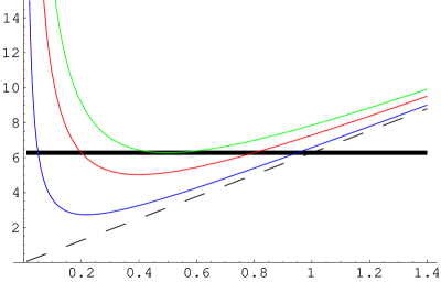
Figure 1: Effective potential for loop motion as a function of $k$. The thick solid line indicates the total conserved energy of the system, measured in units of $m^{2}$. The maximum radius is $r=1$.

As we have noted, in general $k(\eta)$ need not be constant. An example of a loop solution for which this is the case is given by

$${\mathbf{a}}(q)=(\cos q,\sin q,0)\;;\qquad{\mathbf{b}}(\eta)=(0,-\frac{1}{2}\sin\eta,0)\longleftrightarrow k^{2}(\eta)=\frac{1}{4}\cos^{2}\eta,$$ (3.16)

see figure 2. This loop has angular momentum $J=m^{2}\pi/2(<C^{2}/2\pi)$ and does not self-intersect. The figure also indicates one of the two points on the loop for which $k=0$ (and so $|\dot{{\mathbf{x}}}|=|{\mathbf{x}}^{\prime}|=1/2$): this point executes a circular trajectory of radius $1/2$. Below we will see that any loop with this form of ${\mathbf{b}}(\eta)$ does not self-intersect.

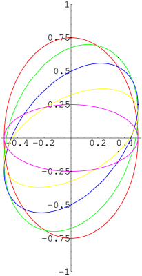
Figure 2: Evolution of the loop given in (3.16) through half a period. At $t=0$ the loop is symmetric about the vertical axis; at $t=L/2=\pi$ it is symmetric about the horizontal axis. Intermediate times increase in steps $\pi/8$. At each time, a point on the loop is labeled by a $\bullet$. This is the point $k=0$ (there are 2 points with $k=0$. The other is not labeled and is diametrically opposite) and it executes a circle of radius $1/2$.

We now study the self-intersection probability of loops with non-constant $k$.

4 Self-intersection properties

The self-intersection probability, $P_{int}$, of loops with given numbers of harmonics on ${\mathbf{a}}$ and ${\mathbf{b}}$ but constant $k$ was studied in [16]. This was done through a simple adaptation of the code of Siemens and Kibble [27] who studied the same question for NG loops (i.e. when $k=1$). Their work was in turn based on methods developed by DeLanley et al [28, 29, 30] who showed how, for a fixed number of harmonics, the Fourier series (3.13) could be generated such that constraint (1.2) is satisfied. Here we use a modified form of the same code to study $P_{int}$ when $k(\eta)$ is not constant.

As seen in section 2.2, $k(\eta)$ can be any periodic function provided $0\leq k^{2}(\eta)\leq 1$. Non-constant $k$ means that the charge per unit length varies along the string and this seems physically reasonable, especially for strings whose length is larger than the horizon or for loops formed as the result of self-intersection of other strings: fluctuations in charge will occur during the phase transition which produces the strings, and charge can be built up in self-intersections.

For non-constant $k(\eta)$, the self-intersection probability $P_{int}$ might be expected to depend on the number of zeros $n_{0}$ in the function $k(\eta)$ (since when $k=0$ the loop never self-intersects), and also on maximum amplitude, $A$, of $k(\eta)$. The dependence of $P_{int}$ on these parameters will be studied.

Unfortunately, once $k\neq$ constant, the freedom in possible loop solutions increases since there is no longer any constraint on the coefficients ${\bf C}_{n}$ and ${\bf D}_{n}$ in the Fourier expansion of $\mathaccent 19{{\mathbf{b}}}$ other than $0\leq\mathaccent 19{{\mathbf{b}}}^{2}\leq 1$. One way to proceed is just to pick out by hand specific functional forms of $k(\eta)$ (of which a constant is just one case) and then try to construct all possible coefficients ${\bf C}_{n}$ and ${\bf D}_{n}$ consistent with that $k(\eta)$, as was done in [28, 29, 30] for constant $k$. One such simple function is

$$k^{2}(\eta)=A^{2}\cos^{2}n\eta\qquad(A<1)$$ (4.1)

which has $2n$ zeros. An example of a non-self-intersecting loop with $n=1$ and $A=1/2$ is shown in figure 2. To see if intersection is possible for any $A$ and $n$ recall that self-intersection occurs if there is a solution to

$${\mathbf{a}}(T+\sigma_{1})+{\mathbf{b}}(T-\sigma_{1})={\mathbf{a}}(T+\sigma_{2})+{\mathbf{b}}(T-\sigma_{2})$$ (4.2)

for some $0<\sigma_{1}\neq\sigma_{2}<L$ and $0<T<L/2$. Let $\chi$ and $\Phi$ be arbitrary angles and consider

$${\mathbf{a}}(q)\!\!\! = \!\!\!\frac{1}{m}(\cos mq,\cos\chi\sin mq,\sin\chi\sin mq),$$

$${\mathbf{b}}(\eta)\!\!\! = \!\!\!\frac{A}{n}(\cos\Phi\sin n\eta,\sin\Phi\sin n\eta,0),$$ (4.3)

which gives $k(\eta)$ as in (4.1). Now let $c=({\sigma}_{1}+{\sigma}_{2})/2$, $\delta=({\sigma}_{1}-{\sigma}_{2})/2$, $q=T+c$ and $\eta=T-c$. Then the self intersection condition (4.2) becomes

$${\mathbf{a}}(q+\delta)-{\mathbf{a}}(q-\delta)={\mathbf{b}}(\eta+\delta)-{\mathbf{b}}(\eta-\delta)$$

for which we must find solutions for $\eta,q,\delta$ with $0<\delta<2\pi$. On substitution of (4.3), this condition becomes

$$\frac{1}{m}(-\sin mq\sin m\delta,\cos mq\sin m\delta\cos\chi,\cos mq\sin m\delta\sin\chi)$$

$$= \frac{A}{n}(\cos\Phi\cos n\delta\sin n\delta,\sin\Phi\cos n\eta\sin n\delta,0)$$

for which the only solution is $\delta=0$. Thus for ${\mathbf{b}}$ given in (4.3) there are no self-intersections.

Let us instead consider a slightly more general form of ${\mathbf{b}}(\eta)$;

$${\mathbf{b}}(\eta)=\frac{A}{n}(\sin n\eta,-\frac{\cos 2dn\eta}{2d}\cos\Phi,-\frac{\cos 2dn\eta}{2d}\sin\Phi)$$ (4.4)

where $d$ is an integer greater than or equal to 1. The corresponding function $k^{2}(\eta)$ once again $2n$ zeros, but the larger $d$ the more oscillations there are in $k^{2}(\eta)$ (figure 3).

Figure 3: Plot of $k^{2}(\eta)=A^{2}(\cos^{2}n\eta+\sin^{2}2dn\eta)$ for $A=1/2$, $n=1$ and $d=1$ (solid line), $d=2$ (dotted line).

The self-intersection condition now becomes (we set $\Phi=0$ for simplicity)

$$\frac{1}{m}(-\sin mq\sin m\delta,\cos mq\sin m\delta\cos\chi,\cos mq\sin m\delta\sin\chi)$$

$$= \!\!\!\frac{A}{n}(\cos n\eta\sin n\delta,\frac{1}{2d}\sin 2dn\eta\sin 2dn\delta,0)$$

which implies that

$$\cos mq=0=\sin 2dn\eta\qquad\Longleftrightarrow\qquad\sin mq=\pm 1=\cos 2dn\eta\qquad(\longleftrightarrow\cos n\eta=0,\pm 1),$$

where $\delta$ must satisfy (for $\cos n\eta\neq 0$)

$$\pm\frac{1}{m}\sin m\delta=\frac{A}{n}\sin n\delta.$$

If $n$ and $m$ have no common factors there are solutions and hence self-intersections.

4.1 Numerical results

The self-intersection probability, $P_{int}$, of loops with ${\mathbf{b}}$ of the form given in (4.4) was studied numerically. For such loops $P_{int}$ is therefore a function of $n_{0}=2n$, $d$, $A$, and also of $N_{a}$, the maximum number of harmonics on the vector ${\mathbf{a}}$. (This vector was generated using the methods of [28]). Note that in this case the charge $C$ is given by

$$C=\frac{m}{2}\oint d\sigma\left[1-A^{2}(\cos^{2}n\sigma+\sin^{2}2dn\sigma)\right]^{1/2},$$ (4.5)

which is essentially independent of the values of $n$ and $d$ for $A\raise 1.29167pt\hbox{$<$\kern-7.5pt\lower 4.30554pt\hbox{$\sim$}}0.5$. Thus for a given charge $C$ on the loop, the dependence of $P_{int}$ on $n$ and $d$ can be investigated, and also compared with the case in which $k$ is constant [16].

Figure 4 shows the dependence of $P_{int}$ on $N_{a}$ for $n=2$ and $d=1$. Each point shown was obtained by generating 10 samples, each containing 100 loops, and looking for self-intersections of each of these loops: the point is the average number of self-intersections, and the error bar is the standard deviation of this mean. This is exactly the procedure used by Siemens and Kibble, and details can be found in their paper. For fixed ${\mathbf{b}}$ (hence fixed charge), the self-intersection probability increases as the number of harmonics in ${\mathbf{a}}$ increases. This is the expected behaviour as the loops are more contorted for larger $N_{a}$. Interestingly $P_{int}$ is only fractionally smaller here than that obtained in [16] for the same charge and constant $k$ (corresponding to $n_{0}=0$).

Figure 4: Self-intersection probability as a function of $N_{a}$, the number of harmonics on ${\mathbf{a}}$. All loops considered have the same charge $C$.

The left-hand plot in figure 5 shows instead the effect of fixing $N_{a}$ (=3) but increasing the number of zeros in $k(\eta)$. The probability $P_{int}$ decreases as expected since each point for which $k=0$ has a very constrained motion. The graph shows results for three different values of $A$ (or equivalently $C$): as $C$ increases, $P_{int}$ decreases — for a given $C$, the self-intersection probability of a loop depends on the form of $k(\eta)$. The right-hand plot of figure 5 is similar to the left-hand plot, and shows how, for fixed $C$, $P_{int}$ increases with $N_{a}$ but decreases with $n$. These effects are equally strong, in that if $N_{a}$=$n$, $P_{int}$ tends to a constant value. For comparison the results obtained in [16] for constant $k$ are plotted also.

Finally, we investigated the dependence of $P_{int}$ on $d$. Figure 6 shows that for fixed $n$, $A$ and $N_{a}$, the self-intersection probability initially decreases as $d$ increases but then seems to have an upturn. We are unable to explain this behaviour at present.

Figure 5: a) This figure shows how, for a given charge $C$ (determined by $A$), the self-intersection probability decreases with $n$. b) The dependence on $N_{a}$ and $n$ for fixed $C$. For comparison we have also plotted the results obtained in [16] for constant $k$ (upper circle: $N_{a}$=25, lower circle $N_{a}$=11).

Figure 6: Dependence of $P_{int}$ on $d$.

5 Conclusions

In this paper we have attempted study and clarify a number of points regarding the evolution and gravitational properties of chiral cosmic strings. As was summarized in section 2, the crucial difference between the equations of motion for NG and chiral cosmic strings is the constraint on the vector $\mathaccent 19{{\mathbf{b}}}$: for NG strings $\mathaccent 19{{\mathbf{b}}}^{2}(\eta)=1$ $\forall\eta$, whereas for chiral strings $\mathaccent 19{{\mathbf{b}}}^{2}(\eta)(=k^{2}(\eta))\leq 1$. Equation (2.11) shows that $k^{2}(\eta)$ determines the charge on the chiral string.

We saw in section 3.1 that chiral strings with $k=0$ ($\forall\eta$) move along themselves and never self-intersect. If the string forms a loop, the energy of this arbitrary shaped vorton is equipartitioned between tension and angular momentum. The charge on the vortons is given by $C=mL_{{\rm phys}}$ where $L_{{\rm phys}}$ is the constant physical length of the vorton.

Infinite straight chiral strings were studied in section 3.2. We saw that the energy momentum tensor contains non-diagonal terms $T^{tz}\neq 0$. These represent the momentum along the string. Furthermore, $T^{tt}\neq T^{zz}$ (if $k\neq 1$) which is reminiscent of the situation which occurs with wiggly NG strings. As a consequence of the form of $T^{\mu\nu}$, the weak-field metric around the string was shown to contain a $dt\,dz$ term which means that photons (and relativistic particles) moving near the string are dragged in the direction of the string. We also observed that there is a $k$-dependent deficit angle as well as a $k$-dependent Newtonian potential.

Regarding the evolution of a chiral cosmic string network (which could formed at the end of D-term inflation), it is important to understand whether or not the loops can self-intersect and then decay. If they cannot decay, this would lead to a cosmological catastrophe as they would dominate the energy density of the universe. In section 3.3 we studied the effective potential for the motion of a non self-intersecting circular loop for which $0\leq k<1$. In section 4 we considered loops with non-constant $k$: the physical reason for which one might expect $k$ not to be constant is that charge will build up as a result of self-intersections, and also fluctuate during the phase transition which forms the string. Analysis of specific form of $k(\eta)$ (given via (4.4)) showed that self-intersection is possible for these loops. The ensuing numerical analysis showed that the self-intersection probability depends on the form of $k(\eta)$ and is not uniquely determined by the charge $C$ of the loop. This unfortunately suggests that even if one were able to estimate $C$ for the strings in a chiral cosmic string network, this would not be sufficient to determine the self-intersection properties of the loops. As a further problem it still remains to understand the fate of the daughter loops.

A number of interesting questions remain to be studied. Regarding the metric (section 3.2), it would be interesting to go beyond the weak-field approximation and also to study carefully the potential cosmological consequences of the $dt\,dz$ term [23]. This cross-term is the main difference between the metric for NG and chiral strings. Concerning the evolution of a network of chiral cosmic strings it is clear that if the network is formed with $k(\eta)=0$ $\forall\eta$ and for all strings, then this leads to a cosmological catastrophe: this is the only case in which the answer for $P_{int}$ is unique and zero! — the strings cannot self-intersect and are frozen. Similar problems occur if this state is reached at anytime during the evolution of the network. This vorton problem was studied in [31] where it was noted that the quantum number $C$ should be larger for chiral strings than for strings with time- or space-like currents. However, work still needs to be done to see if $C$ is maximal or not [32]. If it is not maximal (i.e. $k\neq 0$ $\forall\eta$) it still remains to understand the ultimate fate of the daughter loops, and hence that of the network itself.

References

- [1] A.Albrecht, R.A.Battye and J.Robinson, Phys. Rev. Lett. 79 (1997) 4736; Phys. Rev. Lett. 80 4847 (1998).
- [2] C.Contaldi, M.Hindmarsh and J.Magueijo, Phys. Rev. Lett. 82 (1999) 679.
- [3] P. Avelino et al, Phys. Rev. Lett. 81 (1998) 2008; P.Wu et al, astro-ph/9812156.
- [4] L.Pogosian and T.Vachaspati, Phys. Rev. D60 (1999) 083504.
- [5] E.J.Copeland, J.Magueijo and D.A.Steer, Phys. Rev. D61 (2000) 063505.
- [6] U-L.Pen, U.Seljak and N.Turok, Phys. Rev. Lett. 79 (1997) 1611.
- [7] R.Durrer, M.Kunz and A.Melchiorri, Phys. Rev. D59 (1999) 123005.
- [8] E. Witten, Nucl. Phys. B249 (1985) 557.
- [9] R. Jeannerot, Phys. Rev. D56 (1997) 6205.
- [10] S.C. Davis, A.C. Davis and M. Trodden, Phys. Lett. B405 (1997) 257.
- [11] for example C. Contaldi, M. Hindmarsh and J. Magueijo, Phys. Rev. Lett. 82 (1999) 2034, R.A. Battye and J. Weller, Phys. Rev. D61 (2000) 043501.
- [12] C.J.A.P. Martins and E.P.S. Shellard, Phys. Rev. D57 (1998) 7155.
- [13] S.C.Davis, W.Perkins and A.C.Davis, Phys. Rev. D62 (2000) 043503.
- [14] D.A.Steer, Strings after D-term inflation: evolution and properties of chiral cosmic strings, astro-ph/0010295.
- [15] B. Carter and P. Peter, Phys. Lett. B466 (1999) 41.
- [16] A.C. Davis, T.W.B. Kibble, M. Pickles, and D.A. Steer, Phys. Rev. D62 (2000) 083516.
- [17] J.J.Blanco-Pillado, K.D.Olum and A.Vilenkin, General solution for chiral current carrying strings, astro-ph/0004410.
- [18] B. Carter, P. Peter and A. Gangui, Phys. Rev. D55 (1997) 4647.
- [19] P.Peter and D.Puy, Phys. Rev. D48 (1993) 5546.
- [20] M.J.Thatcher and M.J.Morgan, Phys. Rev. D58 (1998) 043505.
- [21] R.J.Gleiser and M.H.Tiglio; Phys. Rev. D61 (2000) 104006.
- [22] M.J.Thatcher and M.J.Morgan, Phys. Rev. D62 (2000) 103514.
- [23] D.A.Steer and T.Vachaspati, in progress.
- [24] S.Weinberg, Gravitation and Cosmology, John Wiley and Sons, (1972).
- [25] A.Vilenkin, Phys. Rev. D23 (1981) 852.
- [26] see for example M.B.Hindmarsh and T.W.B.Kibble, Rep. Prog. Phys. 58 (1995) 477.
- [27] X.A. Siemens and T.W.B. Kibble, Nucl. Phys. B438(1995) 307.
- [28] D. DeLaney, K.Engle and X. Scheick, Phys. Rev. D41 (1990) 1775.
- [29] R.W. Brown and D.B. DeLaney, Phys. Rev. Lett. 63 (1991) 1674.
- [30] R.W. Brown, M.E. Convery and D.B. DeLaney, J. Math. Phys. 32 (1991) 1674.
- [31] B.Carter and A.C.Davis, Phys. Rev. D61, 123501 (2000).
- [32] A.C.Davis and M.Pickles, in progress.