Interstellar Turbulence:
I. Retrieval of Velocity Field Statistics

Abstract

We demonstrate the capability of Principal Component Analysis (PCA) as applied by Heyer & Schloerb (1997) to extract the statistics of turbulent interstellar velocity fields as measured by the energy spectrum, $E(k)\sim k^{-\beta}$. Turbulent velocity and density fields with known statistics are generated from fBm simulations. These fields are translated to the observational domain, T(x,y,v), considering the excitation of molecular rotational energy levels and radiative transfer. Using PCA and the characterization of velocity and spatial scales from the eigenvectors and eigenimages respectively, a relationship is identified which describes the magnitude of line profile differences, ${\delta}v$ and the scale, $L$, over which these differences occur, ${\delta}v\sim L^{\alpha}$. From a series of models with varying values of $\beta$, we find, $\alpha=0.33\beta-0.05$ for $1<\beta<3$. This provides the basic calibration between the intrinsic velocity field statistics to observational measures and a diagnostic for turbulent flows in the interstellar medium. We also investigate the effects of noise, line opacity, and finite resolution on these results.

1 Introduction

The evolution of the cold, dense interstellar medium and the formation of stars are regulated by the kinetic energy content of turbulent gas flows. Such chaotic motions play a critical role in the equilibrium of the gas as these provide a countering pressure to self gravity and the pressure of the external medium. In the absence of external pressure fronts, the formation of stars occurs exclusively in dense, localized regions where the turbulent energy is sufficiently reduced to enable gravitational collapse. Therefore, an understanding of the dense interstellar medium and the formation of stars requires an accurate description of turbulent gas flow including energy injection into and dissipation from the gas system and the distribution of turbulent kinetic energy over varying spatial scales.

Turbulent flows within the molecular interstellar medium are recognized as observed supersonic line widths and morphological complexity (Scalo 1990; Falgarone Phillips, & Walker 1991). While these observations denote the presence of turbulence in the interstellar medium, there is little quantitative information as to the nature of the turbulent flows. Ideally, one would like to recover the 3-dimensional velocity field, $v_{z}(x,y,z)$, for the line of sight component, z, from a set of spectroscopic observations. In practice, the reconstruction of the true velocity field from observations is not possible given the chaotic, non-deterministic nature of turbulent flows and the non-linear transformation of the field onto the spectroscopic axis of the observer. Therefore, it is essential to construct statistical descriptions of turbulence (Dickman 1985). The primary statistic used to distinguish turbulent models is the energy spectrum, E(k), which describes the degree of coherence of the velocity field over spatial scales. In D dimensions, the energy spectrum is the angular integral of the power spectrum,

$${E(k)=\int d\Omega P(k)\propto<P(|k|)>_{\Omega}k^{D-1}}$$

We refer to the spectral index $\beta$ in connection with E(k),

$${E(k)\sim|k|^{-\beta}}$$

The power spectrum then has the form (in D dimensions) :

$${P(k)\sim|k|^{-(\beta+(D-1))}}$$

For a dissipationless cascade of energy through an incompressible fluid, $\beta=5/3$ and the power spectrum, P(k), decreases in 3 dimensions as k^-11/3 (Kolmogorov 1941). A 2 or 1 dimension cut through the 3 dimensional structure will also have an energy spectrum with the same index $\beta$ but with a different slope of the power spectrum.

The mean square turbulent velocity, $v_{l}$, at size $l$, is determined from the spectrum of velocity fluctuations over scales smaller than $l$,

$$v_{l}^{2}\sim\int_{2\pi/l}^{\infty}E(k)dk\propto\int_{2\pi/l}^{\infty}k^{-\beta}dk\propto l^{\beta-1}$$

$v_{l}^{2}$ describes the variance of the 3 dimensional velocity field, v(x,y,z) within a volume $l^{3}$. The root mean square turbulent velocity, $<v_{l}^{2}>^{1/2}$, is then,

$$<v_{l}^{2}>^{1/2}\propto l^{(\beta-1)/2}=l^{\gamma}$$

where $\gamma=(\beta-1)/2$. It is not equivalent to an observed width of a spectral line which depends upon the velocity, density, temperature, and abundance which vary along the line of sight. However, given a velocity field described by an energy spectrum with $\beta>0$, one might expect some correlation of measured velocities, ${\delta}v$, with projected spatial scale, L, of the form,

$${\delta}v\sim L^{\alpha}$$

where $\alpha$ refers to the measured spectral index in contrast to the intrinsic index $\gamma$ in equation (1.5). Conventionally, ${\delta}v$ has been derived from measured line width or the displacement of centroid velocities of spectral lines.

Coarse limits to values of $\beta$ appropriate for the molecular interstellar medium can be inferred from the early models of observed CO line profiles. To account for the broad velocity widths and the ability of the high opacity CO lines to detect the warm molecular gas located deep within the Orion cloud, Goldreich & Kwan (1974) modeled line profiles with a purely systematic velocity field replicating collapsing motions. For such smooth, systematic velocity fields, $\beta\approx 3$. However, it is unlikely that all molecular clouds undergo global gravitational collapse since this predicts too large a star formation rate in the Galaxy (Zuckerman & Evans 1974). Other systematic velocity fields such as rotation are not observed over the extended scales of molecular clouds (Arquilla & Goldsmith 1984). These results suggest $\beta$ must be smaller than 3. A lower limit to $\beta$ is provided by the inability of purely random velocity fields ($\beta$ = -2 in 3D) to reproduce observed line profiles (Leung & Lizst 1976; Dickman 1985). Given these considerations, an approximate range to the spectral index of the energy spectrum is $3/2<\beta<5/2$.

More direct measures of $\beta$ rely on the identification of a size-line width relationship and the assumption that variations along the spectroscopic axis accurately reflect variations within the intrinsic velocity field. Using a set of inhomogeneous data from the literature, Larson (1981) determined a relationship between the global velocity dispersion, $\sigma_{v}$, and size, L, for a sample of 46 molecular regions in the solar neighborhood, $\sigma_{v}\sim L^{0.38}$. Using a more homogeneous sample of observations, Solomon etal (1987) identified a relationship with an index of 0.5. However, the applicability of these observed relationships to the energy spectrum associated with interstellar turbulence (equation (1.5)) is weak unless one considers the targeted clouds as part of singular, global fluid within the Galaxy (see Dickman 1985). Given the wide range of distances and location of the clouds within different spiral arms, such an assumption is clearly invalid. Rather, these respective relationships derived from a sample of unrelated clouds provide a statement of self gravitational equilibrium if one assumes that the mean column density of clouds is approximately constant. That is, there is a sufficient amount of mass distributed within the cloud to bind the internal turbulent motions.

Several investigations have decomposed spectroscopic data cubes of ¹³CO   or C¹⁸O  emission from targeted molecular clouds into discrete units or “clumps” based on some preassigned definition (Carr 1987; Stutzki & Gusten 1990; Williams, de Geus, & Blitz 1994). For each clump, a global velocity dispersion and size are determined. However, the resultant size-line width relationships show a large scatter and little significant correlation. This may reflect that the localization of emission within a spectroscopic data cube may not uniquely originate from a discrete clump localized in space. Also, the process of identifying clumps limits the resolution to the size of the smallest object.

Scalo (1984) and Kleiner & Dickman (1985) proposed the use of structure and autocorrelation functions of centroid velocity images derived from spectroscopic data cubes. This assumes that the 2 dimensional projection retains the statistical characteristics of the 3 dimensional velocity field. These correlation methods have been applied by Miesch & Bally (1994) to a sample of 12 molecular regions imaged in ¹³CO   emission. The structure functions are described by a power law with a spectral index of 0.86 which corresponds to $\alpha$=0.43 as in equation (1.6). However, these correlation methods are limited. For many regions in the molecular ISM, observed line profiles exhibit non-gaussian shapes for which the centroid velocity is not an accurate approximation. Also, the centroid velocity is not well defined near the edges of the clouds where the signal is weak. Finally, the relationship between the measured value of $\alpha$ and the intrinsic velocity field statistics, $\gamma$ or $\beta$, has not yet been established.

Recently, Heyer & Schloerb (1997, hereafter HS97) motivated the use the multivariate technique of Principal Component Analysis (PCA) to decompose spectral line imaging observations of molecular clouds. From the analysis, they identify a relationship which describes the magnitude of velocity differences of line profiles and the spatial scale at which these differences occur within the image. For several molecular clouds, they find $\alpha\sim 0.4-0.5$. However, it has not yet been demonstrated that this analysis, or the other methods described above, are sensitive to varying field statistics ($\beta$) nor has the relationship between $\alpha$ and $\beta$ been established. Given the complex transformation of the velocity field to the observed spectral axis, one can not assume that $\alpha=\gamma=(\beta-1)/2$.

In this paper, we quantitatively evaluate the ability of PCA to characterize intrinsic velocity fields from spectral line observations. Guided by theoretical and observational results, 3 dimensional models of velocity and density fields with known statistical properties are generated. Observations of these fields are simulated, accounting for non-LTE excitation and radiative transfer. The simulated observations are analyzed with PCA under a variety of physical conditions and observational limitations. We demonstrate that the method is indeed sensitive to velocity fields with varying energy spectra and derive the appropriate calibration between the observed quantity $\alpha$ and $\beta$. In a companion paper (Brunt & Heyer 2000), we use these results to derive the energy spectra for molecular regions in the outer Galaxy.

2 Construction of Model Turbulent Clouds

2.1 Velocity Field Generation

To evaluate the sensitivity of the method outlined by HS97 to varying velocity field statistics, we construct 3 dimensional model velocity fields with prescribed energy spectra. Fields which exhibit varying degrees of spatial correlation can be generated from “colored noise” or fractional Brownian motion (fBm) simulations (Voss 1988; Stutzki et al.  1998). These simulations are not solutions to the fluid equations but rather, are expedient numerical tools with well defined spatial statistics. The resultant fields are oversimplifications of real interstellar velocity fields in which one expects shock structures, intermittency and other complex features.

We use the simplest version of an fBm vector velocity field, in which the components are generated independently. For this type of field there is a roughly equal amount of power between the divergence free (solenoidal) and the curl free (compressible) components. Our model velocity fields are thus somewhat more extreme (in terms of the energy fraction in the compressible modes) than what may be expected for ’typical’ turbulent fields which tend to have their energy spectra dominated by the divergence-free component. The effects, if any, of differing energy fractions in each mode will be the subject of a future paper.

The model velocity field generation is a straightforward process which exploits the Fourier space implementation of fBm in three dimensions. The three steps to generate the v(x,y,z) field are: (1) distribute delta-correlated (Gaussian) noise on a cubic grid of N $\times$ N $\times$ N pixels. In this study, we use N=128; (2) Fourier transform this field to the frequency domain, filter the Fourier space field to the desired power law energy spectrum of spectral index $\beta$, and transform back to the real space domain; (3) Normalize the field to the desired variance, $\sigma_{v}^{2}$. In this study, all velocity fields are normalized such that $\sigma_{v}^{2}=1$. Only one component of the vector velocity field, the observable line-of-sight component $v_{z}(x,y,z)$, is generated. For our analysis, we consider purely isotropic fields. This means that the longitudinal gradients $\delta v_{z}/\delta z$ are statistically equivalent to the transverse gradients ($\delta v_{z}/\delta x$ and $\delta v_{z}/\delta y$).

Ten realizations of v(x,y,z) fields are generated for each of several values of $\beta$ (1.0, 1.5, 2.0 ,2.5, 3.0, 4.0). The input noise for each realization has a unique random number seed. Representative one-dimensional cuts through fields with varying energy spectra generated by this method are displayed in Figure 1. It is clear that as $\beta$ increases, the velocity field becomes smoother and similar to a linear gradient.

2.2 Real-Space Velocity Field Statistics for Model Fields

To ensure that the generated fields have the desired real-space statistics (i.e. $\gamma$), we made direct (real-space) measurements on the generated fields. Of course, it would be possible to construct full-resolution autocorrelation functions or structure functions but without the use of the Fourier Transform, these would be lengthy calculations. We would like to avoid the use of Fourier space in checking the fields, since these were created within the Fourier domain. There is also the requirement that the correct normalization for the measurements be found. To check the real-space statistics, we calculate a variant of the standard (second order) structure function $S(\tau)$,

$$S(\tau)=<(v(r)-v(r+\tau))^{2}>$$

where the angle brackets indicate averaging over all points separated by lag $\tau$. We seek the desired dependence

$$S(\tau)\propto\tau^{2\gamma}$$

$S(\tau)$ can be usefully approximated via coarse-grained versions of the original field (Brunt 1999 and references therein). Specifically, the field v is partitioned into an ensemble of cubical boxes of L pixels on a side, over which v is averaged. This procedure is carried out for dyadic values of L (1, 2, 4, 8, 16, 32, 64), where L=1 corresponds to the original field. For each coarsened version of the field, the mean square difference along the cardinal directions between adjacent coarse pixels is calculated, providing an estimate of S($\tau$ = L). The coarse structure function

$$S_{C}(L)=<(v_{L}(\mbox{\boldmath$r$})-v_{L}(\mbox{\boldmath$r+L$}))^{2}>$$

where v_L is a coarse-grained field. From these measurements the exponent $\gamma$ is obtained via the proportionality

$$S_{C}(L)\propto L^{2\gamma}$$

The ensemble coarse structure function, $<S_{C}(L)>$, is formed by equal weight averaging of all S_C(L) measurements at each L for each set of ten fields at each $\beta$. These ensemble measurements are shown in Figure 2, The deficit at L=64 is partly caused by the periodicity of the fields. A power law is fit to $<S_{C}(L)>$ for L $\leq$ 32 to determine an ensemble value, $\gamma_{E}$, for each $\beta$. Also, a mean value, $<\gamma>$ is derived from the average of all $\gamma$ values obtained individually at each $\beta$. These results are summarized in Table 1. It is clear that the calculated values of $\gamma$ are equivalent to the expected value $(\beta-1)/2$, derived from the input value of $\beta$. In Figure 3, we show the variation of $\gamma_{E}$ with the intrinsic value of $\beta$. For velocity fields with $\beta\geq 3$, we find that $\gamma$ asymptotically approaches unity. This is due to the rapid decrease of the power spectrum such that only the $|$k$|$ $=1$ components are significant. Therefore, the field is similar to a smooth linear gradient. In a recent study, Myers & Gammie (1999) derive a similar conclusion. The lower values of $\gamma_{E}$ and $<\gamma>$ relative to the expected values for the larger $\beta$ values are likely caused by the periodicity requirement, which suppresses the out-of-band (large-scale) gradients, and also partly due to the gradients which result from stochastic fluctuations of the power in the first two wavenumbers. That is, an excess of power at the first wavenumber cannot make the field more smooth (higher $\gamma$), but a deficit of power at this wavenumber can make the field less smooth (lower $\gamma$). A better approximation to “absolutely smooth” fields requires the extension to $\beta=4$.

2.3 Density Field Generation

We consider two forms of the density field. The basic calibration is established with a uniform density field, $n_{\circ}(x,y,z)$=constant. However, to provide a more realistic observation, an inhomogeneous density field is also considered. Since the spatial variation of density corresponds to varying excitation of the trace molecule, these inhomogeneous models are used to to investigate the effects of non-uniform sampling of the velocity field. Recent hydrodynamical models for an isothermal gas show a lognormal density probability density function, PDF (Padoan et al 1997; Passot & Vazquez-Semadeni 1998). Additionally, the power spectrum of the density distribution, in the simulations of Padoan et al (1997), is consistent with a power-law form, of spectral slope (in the power spectrum) of $\sim 2.6$ and similar to values determined from observations (Stutzki et al.  1998).

To generate a field that has a lognormal PDF and a power-law power spectrum, we implement a modified version of the fBm method described in Section 2.1. An fBm field with $\beta=1$ is exponentiated which produces a resultant field with the desired statistics (Schertzer & Lovejoy 1987; Pecknold et al.  1993). The $\beta=1$ fBm field serves as $\ln n$ + constant, where the normalizing constant, given the dispersion in the field, determines the mean density. The normalization of the field to a mean density of $n_{\circ}=1$ is obtained by setting $<\ln n>=-\sigma_{\ln n}$, where $\sigma_{\ln n}$ is the global standard deviation of $\ln n$. Note that $\sigma_{\ln n}$ is independent of $n_{\circ}$. Like the fBm velocity fields, the density field is periodic across the cube boundaries. Therefore, the density field is inspected and, if necessary, re-centered to ensure that no major structures lie across the boundary. We emphasize that there is no spatial correlation between the density and velocity fields as one might expect for real clouds in which density fluctuations result from the localized divergence of the velocity field.

2.4 Physical Properties of the Models

In order to calculate realistic opacities, we assign a physical scale to the simulation. For all realizations the linear size of the cube is 20pc. A pixel or cell is 20pc/128=0.156 pc. The mean density for the uniform density field is 100 cm^-3. For the log normal filds, the mean density varies from 10² to 10⁴ cm^-3. The gas is assumed to be isothermal with a kinetic temperature, T_k equal to 20 K. An approximate measure of the global gravitational equilibrium of the models is given by the ratio of kinetic ($\sim 3\sigma^{2}_{v_{z}}\rho_{0}r^{3}$) to gravitational ($\sim G\rho_{0}^{2}r^{5}$) energies

$$3\sigma^{2}_{v_{z}}/G\rho_{0}r^{2}\sim 1.2(100/<n_{H_{2}}>)$$

where we have taken the radius, r= 10 pc. The models do not significantly deviate from gravitational equilibrium although the equilibrium state of the model clouds is not critical to these results.

2.5 Observations of the Models

Given the density and velocity fields and the kinetic temperature, the brightness temperature is determined from the excitation of the chosen gas probe and the radiative transfer of the emission toward the observer’s line of sight. The excitation of the line, parameterized by the excitation temperature, T_ex, and line center opacity, $\tau_{\circ}$, at the position (x,y,z), are determined from a non LTE calculation which accounts for local radiative trapping (Scoville & Solomon 1974). This depends on the local kinetic temperature, density, and N${}_{H_{2}}$X/${\Delta}$v, where N${}_{H_{2}}$ is the molecular hydrogen column density, X is the abundance ratio to molecular hydrogen, and ${\Delta}$v is the local line width. For these simulations, we generate synthetic line profiles of ¹³CO J=1-0 emission, including excitation calculations up to J=5. Constant values of ¹³CO abundance relative to H₂ (1.25 $\times$ 10^-6) and a kinetic temperature (20 K) are assumed. A pixel scale of (20 pc/128) = 0.156 pc gives the H₂ column density within a cell at position (x,y,z) as

$$N_{H_{2}}(x,y,z)=3.08{\times}10^{18}\;n(x,y,z)\;(20/128)\;\;\;cm^{-2}$$

The local line width is determined from the quadrature sum of the thermal velocity for the molecule, c_th, and the gradient of the velocity field at that position

$${\Delta}v(x,y,z)=\sqrt{c_{th}^{2}+({{\partial v(x,y,z)}\over{\partial z}}{\delta}z)^{2}}$$

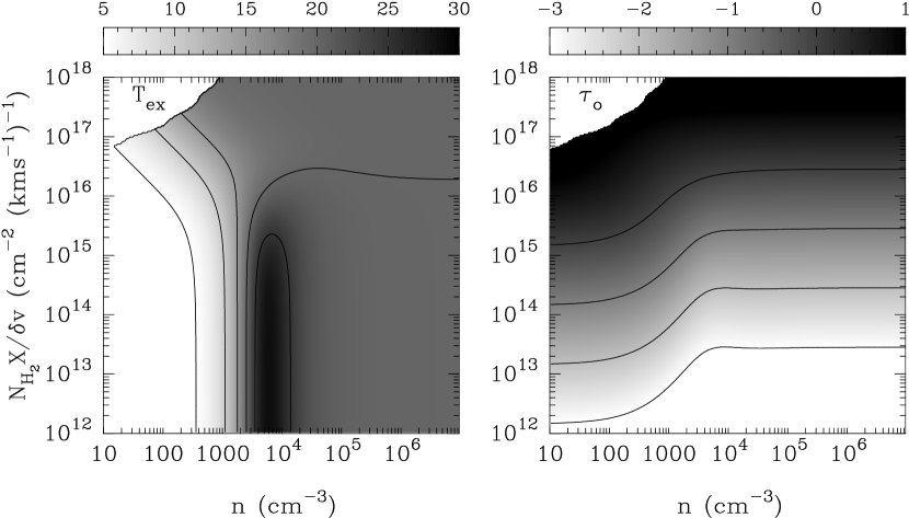
Figure 4: Dependence of $T_{ex}$ (left) and $\tau_{\circ}$ (right) on the local (pixel) density, column density and velocity gradient. The $\tau_{\circ}$ wedge is log₁₀arithmic.

Figure 4 shows the variations of excitation temperature and line center opacity with density and N${}_{H_{2}}$X/${\Delta}$v for the assumed kinetic temperature of 20 K. Once the excitation temperature and line center opacity are determined for each point in the cloud, the emergent intensity at velocity, $v$, is calculated for each position (x,y)

$$T(x,y,v)={{c^{2}}\over{2k\nu^{2}}}\sum_{z=0}^{L_{z}}(B_{\nu}(T_{ex})-B_{\nu}(2.7))(1-e^{-{\tau_{\circ}}\phi(v(x,y,z),{\Delta}v)})e^{-{\Upsilon}(x,y,z,v)}$$

where B_ν(T) is the Planck function, $\nu$ is the line frequency, $\phi$(v(x,y,z),${\Delta}$v) is the Gaussian profile function normalized to unity and

$$\Upsilon(x,y,z,v)=\sum_{\zeta=0}^{z}\tau(x,y,\zeta)\phi(v(x,y,\zeta,{\Delta}v))$$

is the total foreground opacity to a physical depth z. The model cloud is placed at a distance of 1 kpc and is observed with a top-hat telescope beam response which covers 1 pixel or an effective angular resolution of 32.4”. The spectral resolution of the observation is 0.05 kms^-1. Examples of the synthetic observations can be found in Brunt (1999).

3 Analysis

The formal goal of PCA is to determine the set of orthogonal axes such that the data, when projected onto these axes, maximizes the variance. In practice, for spectroscopic imaging observations, it effectively identifies differences in line profiles as these contribute to the variance of the data cube. Such line profile differences can arise from dynamical processes within the gas and can be distinguished from the instrumental noise of the data. Therefore, PCA provides a powerful method to identify kinematic variability within the target object. In this section, we describe the PCA technique and subsequent structural analysis to extract the observationally accessible exponent $\alpha$ from spectroscopic imaging observations.

3.1 Principal Component Analysis Method

A spectroscopic imaging observation is comprised of an ensemble of $n=n_{x}{\times}n_{y}$ spectra each with p spectroscopic channels. We write the resultant data cube as $T(x_{i},y_{i},v_{j})=T(r_{i},v_{j})=T_{ij}$ where $r_{i}=(x_{i},y_{i})$ denotes the spatial coordinate of the $i$th spectrum. The covariance matrix S_jk is

$$S_{jk}={{1}\over{n}}\sum_{i=1}^{n}T_{ij}T_{ik}$$

The set of eigenvectors, $u_{lj}$ and eigenvalues are determined from the solution of the eigenvalue equation for the covariance matrix,

$$Su={\lambda}u$$

The eigenvalue, $\lambda_{l}$, corresponds to the amount of variance projected onto its corresponding eigenvector, $u_{l}$. Therefore, the eigenvalues (and corresponding eigenvectors) are reordered from largest to smallest. In this implementation of PCA, we do not explicitly subtract the mean value, $<T_{j}>=\sum T_{ij}/n$ from each channel image. These are effectively removed within the first, ($l=1$), principal component. Note that no spatial information is contained within the eigenvectors, since the ordering of the spatial part of $T_{ij}$ is arbitrary. The eigenvectors $u_{lj}$ are purely spectroscopic and trace the (ordered) sources of variance in the ensemble of observed line profiles. Also, the eigenvectors are orthogonal, which ensures that the information contained within each component is independent information. Similar decompositions can be obtained by other orthogonal function sets such as wavelets or spherical harmonics. The advantage of PCA over these other basis sets is that the orthogonal vectors are determined by the data and not predetermined.

To spatially isolate the sources of variance contained with the $l^{th}$ component, an eigenimage, $I^{l}(r_{i})$, is constructed from the projected values of the data, $T_{ij}$, onto the eigenvector, $u_{lj}$,

$$I^{l}(r_{i})=\sum_{j=1}^{p}T_{ij}u_{lj}$$

It is equivalent to a velocity-integration of T(x,y,v) that is weighted at each channel by the value of the appropriate eigenvector. Since PCA is a linear decomposition, the random noise of the input data can readily be propagated. The variance of projected values due to noise is

$$\sigma_{l}(r_{i})^{2}=\sum_{j=1}^{p}\left[{{\partial I^{l}(r_{i})}\over{\partial T_{ij}}}\right]^{2}\sigma(T_{ij})^{2}=\sum_{j=1}^{p}u_{lj}^{2}\sigma(T_{ij})^{2}$$

Assuming, that $\sigma(T_{ij})$ is constant over the bandpass of the spectrum and recalling that u is orthonormal ($\sum u_{lj}^{2}=1$), the expression reduces to

$$\sigma_{l}(r_{i})=\sigma(T_{ij})$$

Thus, the variance of values projected onto the $l^{th}$ component is equal to variance of the input data. More importantly, one can readily distinguish values within the eigenimage from those due to instrumental noise.

3.2 Characteristic Scale Measurements

For a given component, $l$, the eigenvectors and eigenimages describe the velocities and positions at which the measured line profiles are different with respect to the noise level. Characteristic velocity differences and the spatial scales over which these differences occur are derived from e-folding lengths of the normalized autocorrelation functions (ACFs) of the eigenvectors and eigenimages respectively (Heyer & Schloerb 1997). The raw autocorrelation functions, $C_{V}^{l}(dv)$, $C_{I}^{l}(\tau)$, are calculated directly from the eigenvectors and eigenimages respectively,

$$C_{V}^{l}(dv)=<(u^{l}(v)u^{l}(v+dv)>$$

$$C_{I}^{l}(\tau)=<(I^{l}(r)I^{l}(r+\tau)>$$

However, in this form, the 2 dimensional autocorrelation function contains an additive component, $C_{N}(\tau)$, due to instrumental noise. In Section 3.3, we demonstrate that the noise subtracted autocorrelation function, $C_{I0}^{l}(\tau)=C_{I}^{l}(\tau)-C_{N}(\tau)$ where $C_{N}(\tau)$ is the autocorrelation function of noise values of the data.

The characteristic velocity scale, ${\delta}v_{l}$, is determined from the velocity lag at which $C_{V}^{l}({\delta}v_{l})/C_{V}^{l}(0)=e^{-1}$. For the 2 dimensional ACF of the eigenimage, one must additionally correct for the effects of finite resolution observations upon the zero lag (see Section 3.4). We determine the spatial correlation lengths along the cardinal directions, ${\delta}x_{l},{\delta}y_{l}$, from the noise corrected ACF,

$${{C_{I0}^{l}({\delta}x_{l})}\over{C_{I0}^{l}(0)}}=e^{-1}$$

$${{C_{I0}^{l}({\delta}y_{l})}\over{C_{I0}^{l}(0)}}=e^{-1}$$

and assign the biased characteristic spatial scale, $L_{lB}$ to the quadrature sum,

$$L_{lB}=\sqrt{{\delta}x_{l}^{2}+{\delta}y_{l}^{2}}$$

As discussed in Section 3.4, the true characteristic scale, $L_{l}$, is derived from the $L_{lB}$ with subpixel corrections to account for finite resolution of the observations. Since the eigenimages tend to be isotropic, the ACF profiles along the cardinal directions are a reasonable approximation to the variation of the ACF along any arbitrary angle. The characteristic velocity and spatial scales are statistically well defined with respect to the noise as these represent mean values over the full spectrum and field respectively. A measurement error, $\sigma_{{\delta}v}$, to the value ${\delta}v_{l}$ is given by one half the velocity resolution of the spectrometer. For the spatial scale, $\sigma_{L}$ is determined from the quadrature sum of the spatial resolution and the degree of anisotropy, $|{\delta}x_{l}-{\delta}y_{l}|$, in the spatial ACF. The PCA velocity statistic, $\alpha$, is then obtained from the set of ${\delta}v,L$ pairs which are larger than the respective spectral and pixel resolution limits and form the power law relationship

$${\delta}v\propto L^{\alpha}$$

where the unsubscripted quantities refer to the ensemble (${\delta}v_{l},L_{l}$). Note that in the retrieval of each ${\delta}v-L$ pair, PCA incorporates information from the entire data cube such that each pair is well defined.

3.3 Instrumental Noise Effects

All real observations contain a noise contribution. For any analysis, it is critical to evaluate how the noise may affect the result. For the ACF of the eigenvector, the characteristic velocity scale measurements are largely unaffected by instrumental noise due to the limited number of channels (p$<$128). However, for large, 2 dimensional images, the contributions to the ACF due to noise can be significant and must be removed. The observed eigenimage is the sum of a noiseless eigenimage, $I_{0}^{l}(r)$, and a noise contribution, $N(r)$,

$$I^{l}(r)=I^{l}_{0}(r)+N(r)$$

The unnormalized spatial ACF, ($C_{I}^{l}(\tau)$) is

$$C_{I}^{l}(\tau)=<(I^{l}_{0}(r)+N(r))(I^{l}_{0}(r+\tau)+N(r+\tau))>$$

$$C_{I}^{l}(\tau)=C^{l}_{I0}(\tau)+C^{l}_{N}(\tau)+<I^{l}_{0}(r)N(r+\tau)+I^{l}_{0}(r+\tau)N(r)>$$

where C${}^{l}_{I0}$ is the ACF of the noiseless eigenimage and C${}^{l}_{N}$ is the ACF of the noise. The term in brackets measures the correlation between signal and noise. We assume that the signal and noise are uncorrelated and treat this term as zero. Therefore,

$$C^{l}_{I0}(\tau)=C^{l}_{I}(\tau)-C_{N}^{l}(\tau)$$

For Gaussian noise,

$$C_{N}^{l}(\tau)=\left\{\begin{array}[]{ll}\sigma^{2}_{N}&\mbox{ for $\tau=0$}\\ 0&\mbox{ for $\tau\neq 0$}\end{array}\right.$$

We exploit the noise propagation properties of PCA and obtain $\sigma^{2}_{N}$ from several high $l$ eigenimages, which are free of signal. A more general procedure can be followed to remove the noise contributions to the autocorrelation function. The noise ACF, $C^{l}_{N}(\tau)$, can be calculated directly from either channel images within the data cube or high $l$ eigenimages which contain no signal. The noise contribution is removed at each value of $\tau$. This method works well for non-Gaussian noise fields such as those obtained by on the fly mapping or reference sharing observations (Brunt & Heyer 2000).

The noise subtracted ACF, $C^{l}_{I0}$ is well determined even in the presence of relatively high noise levels. If this noise subtraction is not carried out, then C${}^{l}_{I}$ contains a noise spike at the origin, such that the spatial correlation lengths are underestimated. Since the noise contribution relative to the signal is larger for higher $l$ eigenimages, this means that the scale lengths are underestimated in such a way as to lessen the slope $\alpha$ of the of the log(${\delta}v$)-log($L$) relationship. HS97 did not make this correction for the noise contribution. Therefore, the derived values of $\alpha$ obtained by HS97 should be considered as lower limits.

3.4 Correction for Finite Resolution Effects

It is important that the analysis results are independent of the resolution at which the observations are obtained. In this Section we discuss the systematic effects within the ACFs due to finite resolution. We demonstrate in Section 4.4 that the spectroscopic ACFs and the derived velocity scales are not compromised by changing the spectroscopic resolution at which the observations are obtained. However, the eigenimage ACFs are resolution-dependent and require a sub-pixel correction to ensure that the spatial scale measurements are not systematically compromised. In brief, for finite resolution observations, the unnormalized ACF at zero lag, $C^{l}_{I0}(0)$, is underestimated. However, by assuming, or estimating, a shape to the ACF in order to extrapolate to zero lag, one can gauge the amount that the scale length is overestimated and provide a correction to the derived biased scale lengths, $L_{lB}$. The alternative option is to fit a functional form with a “scale” parameter to the ACF. We have found that making small corrections to scales obtained from a biased ACF provides the more stable measurement.

A detailed derivation of the corrections for various functional forms of the ACF is given by Brunt (1999). In brief, the measured value of $C_{I0}(0)$ which is used to normalize the ACF is

$$C_{I0}(0)\approx C(\epsilon L_{pix})$$

where $C(\tau)$ is the true ACF, $L_{pix}$ is the pixel size, and $\epsilon<1$, is a number that depends on the shape of the ACF and the shape of the telescope beam. For eigenimages derived from observations with a top hat beam profile, $\epsilon\approx 0.5$. This underestimation with respect to an ideal ACF applies to the full resolution (128²) eigenimages, since a simulation or observation at any finite resolution necessarily involves omission of variance (i.e. contributions to $C_{I0}$) that would be present in a higher resolution measurement. Fortunately, the degree of underestimation and the associated scale corrections for the 128² eigenimages are small.

The overestimated scale measurement $L_{B}$ obtained from an underestimated ACF, $C_{I0}$, satisfies

$${{C(L_{B})}\over{C_{I0}}}=exp(-1)$$

For a functional form of the true ACF, $C$

$$C(\tau)=exp(-(\tau/L)^{\kappa})$$

where $L$ is the true scale length of the ACF and $\kappa$ parameterizes the shape of the ACF, the biased scale length $L_{B}$ is related to the true scale length $L$ via

$$L\approx(L_{B}^{\kappa}-(\epsilon L_{pix})^{\kappa})^{1/\kappa}$$

with $\epsilon\approx 0.5$. For $\kappa=1$ (an exponential ACF), the correction to all measured scales is $-{\epsilon}L_{pix}\approx-L_{pix}/2$. For a Gaussian beam $-{\epsilon}L_{pix}\approx-0.75L_{pix}$ (Brunt 1999). The form of the ACFs for each observation is estimated from a few low $l$ eigenimages. The corrections are not sensitively dependent on small errors in estimating $\kappa$. The application of these corrections to the measured scale lengths ensures consistency of the results for varying resolutions.

4 Results

Initially, the basic calibration between the observed exponent $\alpha$ and the intrinsic field statistics, parameterized by $\beta$, is established for uniform density fields. Subsequently, we evaluate the ${\delta}v-L$ relationship with respect to the uniform density results using more realistic distributions of interstellar material and observational conditions including instrumental noise and varying resolution.

4.1 Uniform Density Results

Ten realizations of the velocity field are created for each value of $\beta$ ranging from 1.0 to 4.0 according to the prescription given in Section 2.1. The real space statistics of these fields are checked and reported in Section 2.2. Synthetic line profiles of ¹³CO J=1-0 emission are calculated at each position, (x,y), assuming a uniform density (n${}_{H_{2}}$ = 100 cm^-3) and uniform temperature (T_k = 20K) via the LVG radiative transfer method described in Section 2.5. The optical depths in these observations are small and the excitation is subthermal and uniform throughout the field which corresponds to an almost perfectly-sampled velocity field. The resultant data cubes are decomposed using PCA and velocity and spatial scales are estimated from the eigenvectors and eigenimages respectively. These scales define a relationship between the magnitude of velocity differences and the spatial scales at which these differences occur. The relationship is fit to a power law parameterized by the exponent $\alpha$.

Figure 5 shows ${\delta}v-L$ relationships for 6 velocity fields with varying values of $\beta$. The dotted lines mark the spectroscopic and spatial pixel sizes. Uncorrected spatial scales $L_{B}$ and spectroscopic scales ${\delta}v$ are restricted to $>2$ pixels and $>1$ spectroscopic channel respectively (see Section 3.4). The lower $\beta$ simulations are characterized by a fewer number of retrieved ${\delta}v-L$ pairs above the resolution limits since most of the variance is generated at small scales.

In Table 1 and Figure 6 we show the relationship between the mean value of $\alpha$ determined from the ensemble of realizations and the input $\beta$. The plotted error bars reflect the standard deviation of values from this mean. These results show that there is a monotonic relationship between the observed and intrinsic exponents for $\beta<3$ and the method, as described in Section 3, is sensitive to velocity fields with varying statistics. A least squares fit to the $\alpha,\beta$ values for $1\leq\beta\leq 2.5$ gives

$${\alpha=(0.33\pm 0.04)\beta-0.05\pm 0.08}$$

This was obtained with $\alpha$ as the dependent variable. For values of $\beta>3$, the derived values of $\alpha$ show a similar transition to smoothness that was seen in the intrinsic $\gamma$ measurements described in Section 2.2. Equation 4.1 provides the basic calibration between an observable measure of kinematic variability within a data cube and the intrinsic velocity field statistics. The relationship between $\alpha$ and $\beta$ remains an empirical measurement. It surely depends upon the dimensionality of the fields since a recent calibration of this technique to 2 dimensional fields reveals a modified relationship, $\alpha_{2D}\approx\beta_{2D}/4$. Given the extreme complexity of transforming a velocity field onto a spectroscopic axis and the identification of velocity gradients by line profile differences, an analytical description of equation 4.1 is not readily determined.

4.2 Lognormal Density Field Results

The results of the previous Section are an important first step in gaining insight into how PCA retrieves the intrinsic velocity field information. However, a uniform density field is clearly unphysical. To evaluate the method with a more realistic density distribution, lognormal density fields (see Section 2.3) with mean values of 10², 10³, and 10⁴ ${\rm cm}^{-3}$  and velocity fields with $\beta=1,2,3$ are observed. The increase of the mean density corresponds to an increase in gas column density and line center optical depth within a given cell. The primary effect of inhomogeneous density fields is to mask the velocity field from the observer as the low density regions do not sufficiently excite the molecular gas tracer into emission. Figure 7 shows the ${\delta}v-L$ relationships obtained by PCA from these observations for these varying conditions. The results obtained from the uniform density observations with the identical velocity fields are included for comparison. The resultant $\alpha$ measurements are tabulated in Table 2.

For the ${\beta}\geq 2$, the derived values of $\alpha$ are similar to the uniform density exponents although there is a constant offset in the logarithm. In addition, the number of significant components at the largest spatial scales increases with increasing density and optical depth. This is surely due to radiative trapping within a given cell which maintains an elevated excitation temperature in low density regions in which the trace molecule would otherwise be insufficiently excited. This suggests that a molecular gas tracer with moderate to high optical depths, such as ¹²CO, provides a more complete sampling of the velocity field. The $\beta=1$ observations tend to overestimate $\alpha$ relative to the uniform density exponent. In this case, the presence of high frequency velocity fluctuations places many cells along a given line of sight at a common velocity (see Figure 1). Therefore, for optical depths larger than unity, the back side of the cloud is hidden from the observer and the field is undersampled. From these results, we conclude that the velocity field statistics with inhomogeneous density fields can be reliably recovered for $\beta\geq 2$ under a wide range of optical depths but are slightly overestimated for more shallow energy spectra $\beta\sim 1$.

4.3 Effects of Instrumental Noise

Any real observation of the ISM necessarily contains instrumental noise. In this Section, we evaluate the effects of instrumental noise upon the analysis by adding a noise field, N(r,v), to the simulated observations of the lognormal density field ($<n_{H_{2}}>=10^{4}$ cm^-3) with values of $\beta=1,2,3$. The input noise is Gaussian with variance $\sigma^{2}_{N}$. We define $\zeta$ as a gauge of the signal to noise of a data cube,

$$\zeta=\sqrt{{{\sigma^{2}-\sigma^{2}_{N}}\over{\sigma^{2}_{N}}}}={{\sigma_{0}}\over{\sigma_{N}}}$$

where $\sigma^{2}=\sigma^{2}_{0}+\sigma^{2}_{N}$ is the variance of the data cube with noise and $\sigma^{2}_{0}$ is the variance of the same in a noiseless observation. Since PCA generally consolidates all spectroscopic channels with signal within the first principal component and noise in the higher components, $\zeta$ can be calculated from the $l=1$ and $l=p$ eigenvalues,

$$\zeta=\sqrt{{{\lambda_{1}-\lambda_{p}}\over{\lambda_{p}}}}$$

In Figure 8, we show the ${\delta}v-L$ relationships derived from simulations with varying signal to noise ($\zeta=4.0,2.0,1.0$). Also shown are the relationships derived with $\zeta=\infty$ (dotted line). The resultant $\alpha$ measurements are shown in Table 3. The primary effect of noise is to reduce the number of significant components that are detected above the resolution limits as the variance generated by the velocity field which is contained in the higher components are overwhelmed by the variance due to noise. This tends to induce systematic effects at large $\beta$ rather than an increased scatter in the retrieved ${\delta}v-L$ pairs. For most spectral line imaging observations, $\zeta>4$ for which the results are largely unaffected by noise (Brunt & Heyer 2000).

4.4 Resolution Effects

In Section 3.6, we described the necessary corrections to the retrieved spatial scales which minimize the effects of finite resolution observations. In this section, we demonstrate the need and utility for such corrections using the simulated observations with varying resolution. The original simulated observations are comprised of 128 $\times$ 128 spatial pixels. We degrade the resolution of the simulated observation ($\beta=2$ and lognormal density field with $<n(H_{2})>=10^{4}$ cm^-3) by spatial block-averaging. This is a reduction in the number of pixels and is equivalent to observing the simulation at a further distance with a top hat beam. We define $\Lambda_{I}$ as the number of resolution elements across the image. Block averaged versions of this simulated observation are calculated for $\Lambda_{I}=64,32,16$. Further reduction in resolution results in only one detected measurement above the resolution limits. The measurements obtained from these observations, for both uncorrected scales and scales corrected for an exponential ACF ($\kappa=1$) are shown in Figure 9. These plots demonstrate the saturation of retrieved pairs at the limit $L=(1-exp(-1))L_{pix}$, expected for a linear interpolation between unity and zero in the normalized ACF. This feature is characteristic of uncorrelated noise with a true scale length of zero. The uncorrected measurements clearly show steepening due to a uniform scale overestimation as the resolution limit, $L_{pix}$, is approached. It is this steepening that compromises the estimation of $\alpha$. When the corrections are applied to the retrieved spatial scales, the derived values of $\alpha$ are consistent between the varying resolutions. Note that if no corrections are made, then the measured value of $\alpha$ represents an upper limit, obtained with the assumption that there is no sub-pixel inhomogeneity. Measurements on real data will always contain this ambiguity, which can only be resolved by increasing the resolution.

It was stated in Section 3.4 that the velocity scales ${\delta}v$ are unaffected by changing the spectroscopic resolution. To demonstrate this statement, we coarse-grained the velocity axis of the same observation. In analogy to the above discussion of spatial scales, we define $\Lambda_{v}$ as the ratio of the total range in velocity spanned by the spectrometer and the velocity resolution. For the original simulated observation, $\Lambda_{v}=128$. The spatial resolution is fixed at $\Lambda_{I}=128$. The results of the PCA retrievals for these fields are shown in Figure 10. Also shown are scale measurements for a coarse-grained field with $\Lambda_{I}=64$, and $\Lambda_{v}=32$. The spatial scales have been corrected for finite spatial resolution. No corrections have been applied to the retrieved velocity scales. These results shows that the velocity scale measurements with degraded spectral resolution are equivalent to those derived from the full resolution observations.

5 Summary

We have investigated the ability of PCA to recover intrinsic turbulent velocity field statistics from spectral line imaging observations of the molecular ISM, and established a preliminary calibration of the method. The calibration, subject to the limitations of the modeling, identifies a monotonic relationship between the intrinsic $\beta$ values (or equivalently, $\gamma$) and observed exponents ($\alpha$) that characterize the velocity field statistics.

In addition to the simplistic nature of the input density and velocity fields, including the assumption of statistical isotropy and the periodicity feature, the major limitations are the lack of mutual consistency between density and velocity, and the assumption of local excitation in the radiative transfer calculations. However, the simulated lognormal observations are in good visual correspondence with real molecular ISM observations. The retrievals from the low density observations are in close agreement with those from the high density observations. This suggests that the accuracy of the method depends upon the degree to which one samples the velocity field, rather than the details of the radiative transfer. For molecular clouds in particular, highly saturated observations may be more reliable (due to more homogeneous sampling and a greater number of retrieved measurements) and this suggests that ¹²CO is likely to provide the most accurate values of $\alpha$. This method could also be applied to HI 21cm emission which is excited over a wide range of physical conditions.

The sampling effects due to noise, which uniformly masks sources of variance, do not affect the fits for $\alpha$, until very high noise levels are reached. As calibrated, the PCA method is resolution-independent but limited in general by necessary assumptions of sub-pixel homogeneity of the emission field. Independent of our modeled calibration, the robustness of measured $\alpha$ values provide quantitative constraints to simulated observations of velocity and density fields from hydrodynamical calculations. We do stress, however, that the calibration of $\alpha$ to $\beta$ achieved in this paper is strictly only valid for the fBm model velocity fields. More realistic turbulent fields may not adhere as closely to the calibration, and in future we intend to include supercomputer MHD simulations in the PCA calibration.

Empirical measurements of $\alpha$ from real data of course do not depend on the calibration to $\beta$ (or $\gamma$), and such measurements will be reported by Brunt & Heyer (2000) for an ensemble of fields taken from the FCRAO Outer Galaxy Survey. Using the preliminary calibration established here, we obtain constraints on the intrinsic velocity field statistics of the molecular ISM.

This work was supported by NSF grant AST 97-25951 to the Five College Radio Astronomy Observatory.

6 References

Arquilla, R. & Goldsmith, P.F. 1984, ApJ, 279, 664

Brunt, C.M., 1999, Ph.D dissertation, University of Massachusetts

Brunt, C.M. & Heyer, M.H. 2000, in preparation

Carr, J.S. 1987, ApJ, 323, 170

Dickman, R.L. 19815, in Protostar and Planets II, eds. D.C. Black & M.S. Matthews, University of Arizona Press, p. 150

Falgarone, E., Phillips, T.G. & Walker, C.K. 1991, ApJ, 378, 186

Goldreich, P. & Kwan, J. 1974, ApJ, 189, 441

Heyer, M.H. & Schloerb, F.P., 1997, ApJ, 475, 173 (HS97)

Kleiner, S.C. & Dickman, R.L. 1985, ApJ, 295, 466

Kolmogorov, A.N, 1941, Dokl. Akad. Nauk SSR, 30, 301

Larson., R.B., 1981, M.N.R.A.S, 194, 809

Leung, C.M. & Lizst, H.S. 1976, ApJ, 208, 732

Miesch, M.S. & Bally, J., 1994, ApJ, 429, 645

Myers, P.C. & Gammie, C.F. 1999, ApJ, 522, L141

Padoan, P., Jones, J.T. & Nordlund, A.P., 1997, ApJ, 474, 730

Passot, T. & Vazquez-Semadeni, E., 1998, Phys. Rev. E, 58, 4501

Pecknold, S., Lovejoy, S., Schertzer, D., Hooge, C. & Malouin, J.F., 1993, in Cellular Automata : Prospects in Astrophysical Applications, eds. Perdang, J.M. & Lejeune, A., (World Scientific), p. 228

Scalo, J.M., 1984, ApJ, 277, 556

Scalo, J.M., 1990, in Physical Processes in Fragmentation and Star Formation, eds. R. Capruzzo-Dolcetta, C. Chiosi, & A. di Fazio, (Dordrecht: Kluwer), p 151

Schertzer, D. & Lovejoy, S., 1987, J. Geophys. Res., 92, 9693

Scoville, N.Z., & Solomon, P.M., 1974, ApJ, 187, L67.

Solomon, P.M., Rivolo, A.R., Barret, J., & Yahil, A. 1987, ApJ, 319, 730

Stutzki, J. & Gusten, R, 1990, ApJ, 356, 513

Stutzki, J., Bensch, F., Heithausen, A., Ossenkopf, V., & Zielinsky, M. 1998, AA, 336, 697

Voss, R., 1988, in The Science of Fractal Images, Eds. Peitgen, H.O., Saupe, D. (New York:Springer-Verlag)

Williams, J.P, de Geus, E.J. & Blitz, L., 1994, ApJ, 428, 693

Zuckerman, B. & Evans, N.J. 1974, ApJ, 192, L149

Figure 1: Examples of one-dimensional cuts through the 3 dimensional model velocity fields for $1\leq\beta\leq 4$.

Figure 2: Ensemble coarse structure function measurements of the model velocity fields. Major tick marks correspond to powers of ten.

Figure 3: Measured relationship between $\beta$ and $\gamma$ derived from the coarse structure function.

Figure 5: Representative results of the PCA retrieval for the uniform density observations. The dotted lines mark the spatial pixel size and spectroscopic channel width.

Figure 6: Basic calibration of the observable $\alpha$ exponent to the intrinsic exponent $\beta$.

Figure 7: PCA measurements from the observation of the lognormal density field. The dashed lines denote the fits obtained from the observation of the same velocity fields with a uniform density distribution. The solid lines are the fits to ${\delta}v$-L pairs.

Figure 8: PCA measurements from observations of the lognormal density field with varying degrees of gaussian distributed noise.

Figure 9: Spatial resolution effects on the PCA measurements. The $\lambda_{s}=128$ measurements are shown as filled circles, and the labeled lower resolution versions as open circles. The dotted lines mark the ”full” resolution limits and the solid line the lower resolution limits.

Figure 10: Spectroscopic resolution effects on the PCA measurements. The $\lambda_{v}=128$ measurements are shown as filled circles, and the labeled lower resolution versions as open circles. The dotted lines mark the ”full” resolution limits and the solid line the lower resolution limits.

Table 1: Uniform Density Field

$\beta$	$\gamma={{\beta-1}\over{2}}$	$\gamma_{E}$	$<\gamma>$	$\alpha$
1.0	0.0	0.00$\pm$0.03	-0.02$\pm$0.04	0.30$\pm$0.06
1.5	0.25	0.26$\pm$0.02	0.23$\pm$0.04	0.45$\pm$0.03
2.0	0.50	0.50$\pm$0.01	0.48$\pm$0.05	0.62$\pm$0.02
2.5	0.75	0.72$\pm$0.01	0.73$\pm$0.04	0.79$\pm$0.04
3.0	1.00	0.85$\pm$0.02	0.86$\pm$0.05	0.92$\pm$0.04
4.0	1.50	0.93$\pm$0.02	0.94$\pm$0.01	1.02$\pm$0.06

Table 2: Lognormal Density Fields

$\beta$		$\alpha$
	$n=10^{2}$${\rm cm}^{-3}$	$n=10^{3}$${\rm cm}^{-3}$	$n=10^{4}$${\rm cm}^{-3}$
1.0	0.40$\pm$0.01	0.47$\pm$0.01	0.44$\pm$0.01
2.0	0.57$\pm$0.03	0.61$\pm$0.02	0.64$\pm$0.01
3.0	0.92$\pm$0.03	0.97$\pm$0.03	0.92$\pm$0.03

Table 3: Lognormal Density Field with Noise

$\beta$		$\alpha$
		$\zeta=\infty$	$\zeta=4.0$	$\zeta=2.0$	$\zeta=1.0$
1.0		0.44$\pm$0.01	0.45$\pm$0.01	0.41$\pm$0.03	0.48$\pm$0.01
2.0		0.64$\pm$0.02	0.64$\pm$0.03	0.64$\pm$0.02	0.57$\pm$0.02
3.0		0.92$\pm$0.03	0.88$\pm$0.02	0.81$\pm$0.01	0.63$\pm$0.04