From Anisotropy to Omega

Abstract

Following the recent measurement of the acoustic peak by the BOOMERanG and MAXIMA experiments in the CMB anisotropy angular power spectrum, many analyses have found that the geometry of the Universe is very close to flat, but slightly closed models are favoured. In this paper we will briefly review how the CMB anisotropies depend on the curvature, explaining any assumptions we could make and showing that this skewness towards closed models can be easily explained by degeneracies in the cosmological parameters. While it is difficult to give independent constraints on the cosmological constant and/or different forms of dark energies, we will also show that combining CMB measurements with other observational data will introduce new and tighter constraints, like $\Omega_{\Lambda}>0$ at high significance.

1 Introduction

In the most general and simple inflationary scenario [1] the overall present energy density of the universe must be equal to the so-called critical energy density ($\Omega=\rho/\rho_{c}=1$, with $\rho_{c}=3H_{0}^{2}/8\pi G$). In fact, the condition for inflation ($\ddot{a}_{inf}>0$, and so $d/dt(H_{inf}^{-1}/a_{inf})<0$) is precisely that which drives $\Omega(t)$ towards $1$ in the Friedmann equation

$$\Omega(t)-1={k\over{a^{2}(t)H^{2}(t)}}$$ (1)

during the inflationary period. This prediction, however, taken with the standard CDM model of structure formation, is apparently in disagreement with a combined set of observations, such as density-velocity galaxy field comparisons ([14]), pairwise galaxy velocities ([15]), X-ray clusters temperature function evolution ([7], [8]) and velocity dispersions ([9])], which point in favor of a low density universe ($\Omega_{matter}<1$). In order to solve the discrepancy, open ($\Omega=\Omega_{matter}<1$) inflationary models have been proposed ([2], [3] [4]). This type of model highlights limitations on the predictiveness of the inflationary scenario, which is supposed to have the advantage of removing any dependence on initial conditions from our present observable universe. However, even if this picture leads to a more complicated phenomenology, it generally determines $\Omega$ directly from parameters of the physical theory.

On the other hand, another way to keep low-density models compatible with the simplest model of inflation is to introduce a cosmological constant, $\Lambda$, such that $\Omega\equiv\Omega_{matter}+\Omega_{\Lambda}=1$. The presence of such a cosmological constant, which is compatible with all the above observations since they are practically insensitive to it, is also preferred by measurements of the magnitude-redshift relationship in high-redshift type Ia supernovae ([16], [17]). Nonetheless, this ’natural’ solution introduces the cosmological constant problem ([5]) that is perhaps even more acute in inflationary cosmology (see [6] for a review). Thus, an accurate determination of the present overall density parameter $\Omega$, even if not a panacea for the cosmological scenario, is at least extremely important in understanding which theoretical framework could explain the above conflicts.

There is much experimental evidence for the presence of a peak in the CMB angular power spectrum ([18], [19]). Furthemore, with the recent release of the BOOMERanG-98 [20] and MAXIMA-1 [30] spectra, the shape and position of the peak has been detected with unprecedented accuracy. This result, apart from being in wonderful agreement with the standard scenario of primordial adiabatic fluctuations, has important consequences on the parameter $\Omega$ ([33], [37], [38], [39], [40]). As previously noted and already well explained in the literature, the effect of the curvature is to change the relationship between the physical scales on the Last Scattering Surface (LSS) and the corresponding angular scales (see., e.g. [21], [22]). In an open universe, for example, the geodetics focalize in such a way that a particular angular scale will correspond to a greater physical scale on the LSS than the one expected in a flat model. The immediate result is a shift in the radiation angular power spectrum (the so-called $C_{\ell}$’s), and thus a dependence of the position of the first peak $\ell_{peak}$ on the curvature ([41], [23], [24], [25], [26]). The CMB power spectrum is therefore a powerful tool for the determination of the curvature and so of the overall energy density.

Figure 1: The BOOMERanG and MAXIMA $C_{\ell}$’s data together with the most viable open, closed and flat models from present non–CMB observations.

2 $\Omega$ and the shift of the CMB Angular Power Spectrum

In Fig.1, we show the recent data from the BOOMERanG ([19],[20]) and from the MAXIMA [30] experiments together with the predictions of the most viable open, flat and closed adiabatic models (from present non–CMB observations). It is quite evident that the open (closed) model predicts a first peak on smaller (larger) scales with respect to the flat model, which is in much better agreement with the data.

In the literature, the dependence of $\ell_{peak}$ on $\Omega$ is often expressed as

$$\ell_{peak}\sim{220\over\sqrt{\Omega}}$$ (2)

However, this approximation is not correct in $\Lambda$–dominated universes (see Fig.1, where the peak for the closed model is at $\sim 130$ instead of $\sim 190$) and does not take into account the further dependence of $\ell_{peak}$ on other parameters like the Hubble constant and the matter density $\Omega_{m}$. So, in view of the recent $\ell_{peak}=197\pm 6$ ([20]), further modifications to the above formula are needed (see also [27], [28]). Also, the width of the peaks and the inter peak distance vary as functions of $\Omega$ (again see Fig.1) so a more complete expression is needed to describe these effects. This point is rather important because knowing the exact dependence of the CMB spectrum on $\Omega$ will help us in understanding the shape of the probability distribution function for this parameter and, ultimately, how well it can be measured independently.

In order to do this, it is convenient to introduce the ’shift’ parameter $R$ defined as

$$\ell_{peak}=\ell^{flat}_{peak}/{\it R}$$ (3)

where $flat$ indicates the flat, pure–CDM, $\Lambda=0$ model. The use of the $R$ parameter is more appropriate than the conventional $\ell_{peak}$ because it has a clearer geometrical dependence.

As usual, let us assume the metric of space–time to be of a Friedman–Lemaitre–Robertson–Walker (FLRW) form with curvature $k$:

$$ds^{2}=a(t)^{2}[-d\eta^{2}+\gamma_{ij}dx^{i}dx^{j}]$$ (4)

with

$$\gamma_{ij}dx^{i}dx^{j}=dr^{2}+\chi^{2}(r)(d\theta^{2}+sin^{2}\theta\phi^{2})$$ (5)

where the function $\chi(r)$ depends on the curvature $k$ and is $r$, $\sin(r)$ or $\sinh(r)$ for $k=0$ (flat models), $k=1$ (closed models) and $k=-1$ (open models), respectively. The position of the first acoustic peak is determined primarly by the angle subtended by the acoustic horizon $\lambda_{ac}$ at decoupling time, $\eta_{dec}$. The angle under which a given comoving scale $\lambda$ at conformal time $\eta_{dec}$ is seen on the sky is given by $\theta(\lambda)=\lambda/\chi(\eta_{0}-\eta_{dec})$. As the harmonic number $\ell$ is inversely proportional to the angle $\theta$, we have $R=\theta_{ac}/\theta_{ac}^{flat}$, with $\theta_{ac}=c_{s}\eta_{dec}/\chi(y)$, where $c_{s}=1/\sqrt{3(1+3\Omega_{b}/4\Omega_{rad}(1+z_{dec}))}$ denotes the adiabatic sound speed of the baryon/photon plasma at decoupling. It is possible to show that [22]:

$$\eta_{dec}={{2\sqrt{|\Omega_{k}|}}\over{\Omega_{m}}}(\sqrt{\Omega_{rad}+\Omega_{m}/(z_{dec}+1)}-\sqrt{\Omega_{rad}})$$ (6)

where $z_{dec}\sim 1100$ is the redshift at decoupling and $\Omega_{k}=1-\Omega_{m}-\Omega_{\Lambda}$. Furthermore, we have:

$$y=\eta_{0}-\eta_{dec}=\sqrt{|\Omega_{k}|}\int_{0}^{z_{dec}}{{dz}\over{[\Omega_{m}(1+z)^{3}+\Omega_{k}(1+z)^{2}+\Omega_{\Lambda}]^{1/2}}}$$ (7)

For a flat, $\Omega_{m}=1$, $\Omega_{\Lambda}=0$, universe we have

$$\theta_{ac}^{flat}=c_{s}\eta_{dec}/(\eta_{0}-\eta_{dec})=c_{s}(\sqrt{\Omega_{rad}+1/(z_{dec}+1)}-\sqrt{\Omega_{rad}})$$ (8)

We then find, keeping constant $\Omega_{b}h^{2}$ (and so $c_{s}$) and $\Omega_{m}h^{2}$ (see next section) [29]:

$$R={{2\over\chi(y)}}\sqrt{{|\Omega_{k}|\over\Omega_{m}}}$$ (9)

which is a quantity just dependent on $\Omega_{k}=1-\Omega_{\Lambda}-\Omega_{m}$ and $\Omega_{m}$.

Figure 2: $R=constant$ lines in the $\Omega_{\Lambda}-\Omega_{m}$ plane.

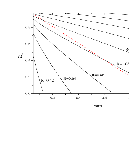
In Fig.2 we plot the contours at $R=const$ in the $\Omega_{\Lambda}-\Omega_{m}$ plane, together with one dashed line such that $\Omega=1$. As we can see, open models have in general $R<1$, while closed models have $R>1$. This is the usual result that in an open model the peaks are shifted towards greater $\ell$ values (smaller angular scales) with respect to the flat model case, while for closed models we have the opposite effect. It is worth noting that the CMB angular shift is not linearly related to the curvature: lines at $\Omega=const$ are not parallel with the $R=const$ contours, but have multiple intersections, especially in regions far from flatness (again, see Fig.2).

In Section 4, we will build a likelihood distribution function $L$ for $\Omega$, using a Bayesian approach to compare the current CMB data with the theoretical predictions and then marginalizing over the remaining cosmological parameters. The above result implies that the probability distribution function for $\Omega$ (if we assume a flat prior distribution on the remaining parameters while marginalizing) will always be ’skewed’ so that $\Omega$ will never be measured at a level better than $10-20\%$.

3 The geometrical degeneracy

With the parameter $R$ fixed, the structure and position of the $C_{\ell}$ spectrum is dependent on $2$ physical scales: the equality scale and the sound horizon at decoupling scale. These quantities are completely defined once we choose the abundance of cold dark and baryonic matter in our model, by the parameters: $\omega_{cdm}=\Omega_{cdm}h^{2}$ and $\omega_{b}=\Omega_{b}h^{2}$. The CMB spectrum also depends on the characteristics of the primordial inflationary perturbations. Assuming that we have already selected the primordial power spectrum of our model, both in shape (tilted or ’blue’) and in nature (adiabatic, isocurvature, hybrid), the structure of the CMB angular peaks is completely determined by $R$, $\omega_{b}$ and $\omega_{m}=\omega_{b}+\omega_{cdm}$. cdm This result has an important consequence: if we let $\Omega_{b}$, $\Omega_{cdm}$ and $h$ assume any value but a fixed $\omega_{m}$ and $\omega_{b}$, the lines at $R=const$ in the $\Omega_{m}-\Omega_{\Lambda}$ plane correspond to sets of degenerate power spectra with an identical shape on subdegree angular scales ($\ell>30$) [29].

Figure 3: Concordance model and degenerate models

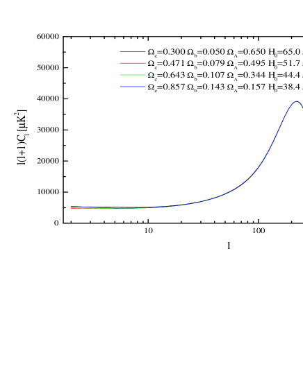
In Fig.3 we draw a set of degenerate models with $R$, $\omega_{m}$ and $\omega_{b}$ set to those of the cosmological concordance model, $\Omega_{m}=0.35$, $\Omega_{\Lambda}=0.65$, $h=0.65$, $\omega_{b}=0.021$, $n_{s}=1$. It is clear from the degeneracy of the models that, once $\Lambda$ is included, the peak position is not directly related to $\Omega$. It is also clear that it seems impossible to obtain any relevant and independent information from the CMB on $\Omega_{\Lambda}$: the Integrated Sachs-Wolfe effect on large scales could in principle break the degeneracy but cosmic variance and a possible presence of a gravity wave background make this effect difficult to disentangle.

Our main results are then the following:

• Lines at $R=const$ in the $\Omega_{\Lambda}-\Omega_{m}$ plane correspond to sets of degenerate $C_{\ell}$ power spectra.

• Given a flat $\Omega_{\Lambda}\sim 0.65$ model, a degenerate closed model can be found by decreasing $\Omega_{\Lambda}$ and $h$ and increasing $\Omega_{b}$ and $\Omega_{cdm}$.

• $R$, $\omega_{m}$ and $\omega_{b}$ are the most meaningful CMB anisotropy observables.

• The CMB spectrum is a useful tool for the determination of $\Omega$ only if we live in a flat universe ($R=const$ are not parallel to $\Omega=const$ when $\Omega$ greatly differs from one).

• Assuming that the concordance model describes our real universe we expect that a likelihood analysis for $\Omega$, using only the CMB power spectrum and without including any external information about $h$, $\Omega_{m}$ and $\Omega_{\Lambda}$, will always be skewed towards closed models.

4 From CMB to $\Omega$

Let us now describe the standard tools for extracting the cosmological parameters from CMB anisotropy observations. Here we will analyze the recent BOOMERanG97 ([19]), BOOMERanG98 ([20]) and MAXIMA ([30]) results. The power spectra from these experiments were estimated in $7$, $12$ and $10$ bins respectively, spanning the range $25\leq\ell\leq 785$. In each bin, the spectrum is assigned a flat shape, $\ell(\ell+1)C_{\ell}/2\pi=C_{B}$. Following [31] we use the offset lognormal approximation to the likelihood $L$. In particular we define:

$$-2{\rm ln}L=(D_{B}^{th}-D_{B}^{ex})M_{BB^{\prime}}(D_{B^{\prime}}^{th}-D_{B^{\prime}}^{ex}),$$ (10)

$$D_{B}^{X}={\rm ln}(C_{B}^{X}+x_{B}),$$ (11)

$$M_{BB^{\prime}}=(C_{B}^{ex}+x_{B})F_{BB^{\prime}}(C_{B^{\prime}}^{ex}+x_{B^{\prime}}),$$ (12)

where $C_{B}^{th}$ ($C_{B}^{ex}$) is the theoretical (experimental) band power, $x_{B}$ is the offset correction and $F_{BB^{\prime}}$ is the Gaussian curvature of the likelihood matrix at the peak. Of course, $C_{B}^{th}$ will depend on the various parameters of our cosmological model ($\omega_{m}$,$n_{s}$, …), and so it will be the likelihood function $L$. In order to compute the likelihood for a given parameter only $\alpha$ we can either marginalize over all the remaining parameters, namely carry out the integral

$$L_{marg}(\alpha)=\int P_{prior}(\alpha,{\vec{\Pi}})L(\alpha,{\vec{\Pi}})d{\vec{\Pi}}$$ (13)

where $\vec{\Pi}$ is a vector containing all the remaining parameters and $P_{prior}$ is the prior probability distribution, or we can maximize i.e. for a fixed $\alpha$ find the ${\vec{\Pi}_{max}}$ wich maximizes

$$L_{max}(\alpha)=P_{prior}(\alpha,{\vec{\Pi}_{max}})L(\alpha,{\vec{\Pi}_{max}}).$$ (14)

The two methods, in general, agree at a level of $\sim 10\%$. The maximization method is usually based on a search algorithm through the second derivative of the likelihood matrix ([32]). In this approach the $C_{\ell}$ spectrum is computed on the way, without sampling the whole parameter space. A different approach is based on building a database of $C_{\ell}$’s on a discretized grid of the parameter space. $L(\Omega)$ is then obtained by maximizing and/or integrating the likelihood computed on the grid ([33], [34]). Of course, producing a grid of models can be quite computationally expensive even with the new and fast boltzmann codes like CAMB [43] or CMBFAST [42]. But this problem can be drastically reduced using morphing [35] or interpolation [36] algorithms.

The definition of the database is rather important because it defines the internal $P_{prior}$ of our analysis and, in general, it is better to have this prior as flat as possible for each given parameter. This brings us to the choice of the variables in which the database must be sampled. As we saw in the previous section, the CMB anisotropies are mainly sensitive to the physical variables $\omega_{i}$ and $R$, so sampling in those variables will avoid degeneracies. Furthemore, the physical baryon density $\omega_{b}=\Omega_{b}h^{2}$ is well determined by independent measurements like primordial nuclide abundances, so this is the optimal choice for extracting information about this parameter (without involving complicated Jacobian transformations) or assume external priors for it. For the same reason, extracting confidence limits on parameters like $h$ can be a little more elaborate with this sampling, being the database in $\sim h^{2}$.

Another possibility is to sample the database in cosmological variables, like $\Omega_{i}$ and $h$. Of course, this will introduce degenerate models in our database but this sampling has the advantage of obtaining direct constraints on the commonly used parameters and with flat prior distributions. In most of the recent papers, either a ’hybrid’ variables approach, with sampling in $\omega_{i}$ and $1-\Omega_{m}-\Omega_{\Lambda}$, or the cosmological variables approach has been used. Here we will choose the database approach, sampling the parameter space in cosmological variables as follows: $\Omega_{m}=0.1,...,1.1$; $\Omega_{\Lambda}=0.0,...,1.0$; $\Omega_{b}=0.01,...,0.25$; $h=0.25,...,0.95$ and $n_{s}=0.50,...,1.50$. We will not consider the possibility of high redshift reionization of the intergalactic medium $\tau_{c}>>0$, a gravity waves contribution or the effect of massive neutrinos.

5 Removing the geometrical degeneracy: Results

Figure 4: Likelihood functions with age prior.

Figure 5: Likelihood functions with $h=0.65\pm 0.2$ and age priors.

Figure 6: Likelihood functions with $\Omega_{m}=0.3\pm 0.2$ prior.

Figure 7: Likelihood functions for a combined analysis with Supernovae.

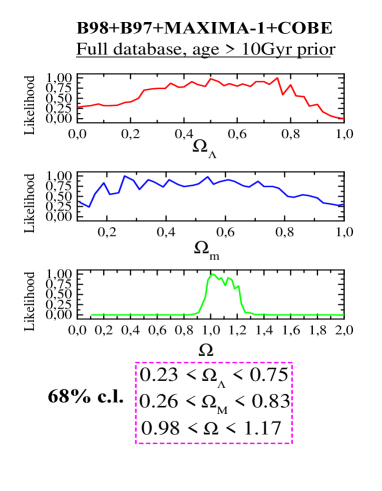
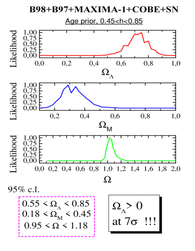
In Fig.4 we plot our likelihood contours for $\Omega$, $\Omega_{m}$ and $\Omega_{\Lambda}$ using just the intrinsic internal priors of the database plus the quite reasonable age prior $t_{universe}>10Gyr$. As we can see, the likelihood for $\Omega$ is skewed towards closed models but is consistent with flatness. It is rather important to note that this skewness is largely due to the $R$-degeneracy which makes ’more’ closed models compatible with the observations. The likelihood for $\Omega_{\Lambda}$ and $\Omega_{m}$ are quite flat due to the geometrical degeneracy but they nonetheless feel border effects from the database priors. The likelihood for $\Omega$ starts to be in even more agreement with flatness when a Gaussian prior $h=0.65\pm 0.2$ is assumed as in Fig.5. This clearly shows that most of the degeneracies in the $h<0.5$ region are well removed by the prior. Including a prior $\Omega_{m}=0.3\pm 0.2$ (Fig.6) as suggested by the majority of measurements, shrinks the likelihood towards $\Omega=1$ and gives a strong determination for the cosmological constant $\Omega_{\Lambda}>0$ at $4\sigma$ level. The complementarity with the supernovae type Ia measurements is even more clear in Fig.7, where a combined CMB+SnIA analysis gives $\Omega_{\Lambda}>0$ at more than $7\sigma$ and $\Omega=1$ with a few percent uncertainty.

6 Conclusions

The BOOMERanG and MAXIMA data support the main prediction of the inflationary paradigm: that the geometry of the universe is flat. The small deviations towards closed models reported in various analyses ([37],[39]) can be easily explained by the degeneracies in the cosmological parameters, which make more closed models compatible with the data. These conclusions are considerably strengthened by the inclusion of other cosmological data such as measurements of the Hubble constant, the overall matter density $\Omega_{m}$ and the accelerating expansion rate indicated by observations of distant Supernovae. At the same time, $\Omega_{\Lambda}$ and other forms of ’dark energy’ cannot be well determined by the CMB data alone, in spite of their high precision. This does not mean that CMB measurement are not useful in the determination of such parameters: combining the CMB data with constraints from observations of large-scale-structure and from observations of SN-Ia increases the extent to which $\Lambda$ can be quantified, with $\Omega_{\Lambda}>0$ at $\sim 7\sigma$. Future data from the PLANCK and/or SNAP satellites will hopefully enable us to resolve the ’dark energy’ puzzle.

Aknowledgements

We would like to thank Monique Signore, Paolo de Bernardis, Marian Douspis, Ruth Durrer, Pedro Ferreira, Graca Rocha, Joe Silk, Filippo Vernizzi and Nicola Vittorio. We also acknowledge using CMBFAST, CAMB and Lloyd Knox’s RADPack [44] packages for the COBE data.

References

- [1] A. Guth, Phys. Rev. D 23, 347 (1981)
- [2] Sasaki M. et al, Phys. Lett. B, 317, 510, 1993
- [3] M. Bucher, A.S. Goldhaber, N. Turok, Phys. Rev. D52, 3314, (1995)
- [4] A. Linde, Phys. Lett. B, 99, 351,(1995)
- [5] S. Weinberg, Rev. Mod. Physics, 61, 1, (1989)
- [6] R.H. Brandemberger, astro-ph/9910410, (1999)
- [7] V. Eke et al, MNRAS, 298, 114, (1998)
- [8] J.P. Henry, ApJ, 534, 565 (2000)
- [9] Carlberg et al, ApJ, 479, L19, (1997)
- [10] S. Colafrancesco, P. Mazzotta, N. Vittorio, Apj, 345, 231, (1998)
- [11] P. Viana and A. Liddle, MNRAS, 303, 535, (1999)
- [12] S. Borgani et al, ApJ, 517, 40, (1999)
- [13] A. Blanchard, R. Sadat, J.G. Bartlett, M. Le Dour, astro-ph/9908037, (2000), A&A, 362, 809
- [14] J. P. Blakeslee, M. Davis, J. L. Tonry, A. Dressler, E. A. Ajhar, astro-ph/9910340, ApJ letters in press (2000)
- [15] R.Juszkiewicz, P.G. Ferreira, H.A. Feldman, A.H. Jaffe, M. Davis, Science, 287, 109, (2000)
- [16] S. Perlmutter et al, Astrophys.J., 517, 565,(1999)
- [17] Riess et al. 1998, AJ, 116, 1009
- [18] A. Miller et al, Astrophys.J. 496, 34, (1999)
- [19] P. D. Mauskopf et al, Astrophys.J., 536, L59-L62, (2000)
- [20] P. de Bernardis, et al, Nature 404, 955-959, (2000)
- [21] S. Weinberg, Gravitation and Cosmology, Wiley, New York, (1972)
- [22] E.W. Kolb and M. S. Turner, The Early Universe, Addison-Wesley, Redwood City, CA, (1990)
- [23] M. Kamionkowski, D. N. Spergel, N. Sugiyama, Astrophys. J. 426, L57, (1994)
- [24] W. Hu, N. Sugyama, J. Silk, Nature, 386, 37-43, (1997)
- [25] W. Hu, M. White, Proceedings of the XXXIth Moriond meeting, astro-ph/9606140, (2000)
- [26] D. Scott, M. White, Astrophys.J., 459, 415, (1996)
- [27] S. Weinberg, astro-ph/0006276, (2000)
- [28] W. Hu, et al, astro-ph/0006436, (2000)
- [29] G. Efstathiou and D. Bond, MNRAS, astro-ph/9807103, (1998)
- [30] S. Hanany et al, astro-ph/0005167, (2000)
- [31] J.R. Bond, A.H. Jaffe & L. Knox 2000, ApJ, 533, 19
- [32] S. Dodelson, L. Knox, Phys.Rev.Lett. 84, 3523 (2000)
- [33] A. Melchiorri et al, ApJL L63, 536, (2000).
- [34] M. Tegmark and M. Zaldarriaga, astro-ph/0004393, (2000)
- [35] K. Sigurdson, D. Scott, New Astronomy, 5, 91-101, (2000)
- [36] M. Tegmark, M. Zaldarriaga, A. J. S. Hamilton, astro-ph/0008167, (2000)
- [37] A. Lange et al, PRD, in press, (2000)
- [38] A. Balbi et al, ApJ, submitted (2000)
- [39] A. Jaffe et al, PRL, in press, (2000)
- [40] R. Durrer, B. Novosyadlyj, (2000)
- [40] A. D. Dolgov, M. V. Sazhin, Ya. B. Zeldovich, “Basics of Modern Cosmology”, Editions Frontieres, (1990)
- [41] J. Silk, M. L. Wilson, Physica Scripta, 21, 708, (1980)
- [42] Seljak, U. & Zaldarriaga, M. 1996, ApJ, 469, 437.
- [43] Lewis A., Challinor A., Lasenby A., astro-ph/9911176
- [44] See the RADPACK home page: http://flight.uchicago.edu/knox/radpack.html