The Dyer-Roeder distance in quintessence cosmology and the estimation of $H_{0}$ through time-delays.

Abstract

We calculate analytically and numerically the Dyer-Roeder distance in perfect fluid quintessence models and give an accurate fit to the numerical solutions for all the values of  the density parameter and the quintessence equation of state. Then we apply our solutions to the estimation of $H_{0}$ from multiple image time delays and find that the inclusion of quintessence modifies sensibly the likelihood distribution of $H_{0}$ , generally reducing the best estimate with respect to a pure cosmological constant. Marginalizing over the other parameters ($\Omega_{m}$ and the quintessence equation of state) , we obtain $H_{0}=71\pm 6$ km/sec/Mpc for an empty beam and $H_{0}=64\pm 4$ km/sec/Mpc for a filled beam. We also discuss  the future prospects for distinguishing quintessence from a cosmological constant with time delays.

I Introduction

Quintessence (Caldwell et al. 1998) or dark energy is a new component of the cosmic medium that has been introduced in order to explain the dimming of distant SNIa  (Riess et al. 1998; Perlmutter et al. 1999) through an accelerated expansion while at the same time saving the inflationary prediction of a flat universe. The recent measures of the CMB at high resolution (Lange et al. 2000, de Bernardis et al. 2000, Balbi et al. 2000) have added to the motivations for a conspicuous fraction of unclustered dark energy with negative pressure. In its simplest formulation (see e.g. Silveira & Waga 1997), the quintessence component can be modeled as a perfect fluid with equation of state

$$p_{q}=\left(\frac{m}{3}-1\right)\rho_{q}$$ (1)

with $m$ in the range $0\leq m<3$ ($m<2$ for acceleration). When $m=0$ we have pure cosmological constant, while for $m=3$ we reduce to the ordinary pressureless matter. The case $m=2$ mimicks a universe filled with cosmic strings (see e.g. Vilenkin 1984). More realistic models possess an effective equation of state that changes with time, and can be modeled by scalar fields (Ratra & Peebles 1988, Wetterich 1995, Frieman et al. 1995, Ferreira and Joyce 1998), possibly with coupling to gravity or matter (Baccigalupi, Perrotta & Matarrese 2000, Amendola 2000).

The introduction of the new component modifies the universe expansion and introduces at least a new parameter, $m$, in cosmology. Most deep cosmological tests, from large scale structure to CMB, from lensing to deep counting, are affected in some way by the presence of the new field. Here we study how a perfect fluid quintessence affects the Dyer-Roeder (DR) distance, a necessary tool for all lensing studies (Dyer & Roeder 1972, 1974). The assumption of constant equation of state is at least partially justified by the relatively narrow range of redshift we are considering, $z\in(0.4,2.5)$. We rederive the DR equation in quintessence cosmology, we solve it analytically whenever possible, and give a very accurate analytical fit to its numerical solution. Finally, we apply the DR solutions to a likelihood determination of $H_{0}$ through the observations of time-delays in multiple images. The dataset we use is composed of only six time-delays, and does not allow to test directly for quintessence; however, we will show that inclusion of such cosmologies may have an important impact on the determination of $H_{0}$ with this method. For instance, we find that $H_{0}$ is smaller that for a pure cosmological constant. In this work we confine ourselves to flat space and extremal values of the beam parameter $\alpha$; in a paper in preparation we extend to curved spaces and general $\alpha$.

II The Dyer-Roeder distance in quintessence cosmology

In this section we derive the DR distance in quintessence cosmology, find its analytical solutions, when possible, and its asymptotic solutions. Finally, we give a very accurate analytical fit to the general numerical solutions as a function of $\Omega_{m}$ and $m$.

First of all, let us notice that when quintessence is present, the Friedmann equation (the $0,0$ component of the Einstein equations in a flat FRW metric) becomes (in units $G=c=1$)

$$\left(\frac{\dot{a}}{a}\right)^{2}=H_{0}^{2}\left[\Omega_{m}a^{-3}+\left(1-\Omega_{m}\right)a^{-m}\right].$$ (2)

where $H_{0}$ is the present value of the Hubble constant, $\Omega_{m}$ the present value of the matter density parameter, and where the scale factor is normalized to unity today. In terms of the redshift $z$ we can write

$$\frac{\dot{a}}{a}=H_{0}E\left(z\right).$$ (3)

where

$\displaystyle E^{2}\left(z\right)=\Omega_{m}\left(1+z\right)^{3}+\left(1-\Omega_{m}\right)\left(1+z\right)^{m}$

The Ricci focalization equation in a conformally flat metric (such as the FRW metric) with curvature tensor $R_{\alpha\beta}$ is (see e.g. Schneider, Falco & Ehlers 1992)

$$\stackrel{{\scriptstyle..}}{{\sqrt{A}}}+\frac{1}{2}R_{\alpha\beta}k^{\alpha}k^{\beta}\sqrt{A}=0$$ (4)

where $A$  is the beam area and $k^{\alpha}=\frac{dx^{\alpha}}{dv}$ is the tangent vector to the surface of propagation of the light ray, and the dot means derivation with respect to the affine parameter $v$. Multiplying the Einstein’s gravitational field equation $R_{\alpha\beta}-\frac{1}{2}g_{\alpha\beta}R=8\pi T_{\alpha\beta}$ by $k^{\alpha}k^{\beta}$ and imposing the condition $g_{\alpha\beta}k^{\alpha}k^{\beta}=0$ for the null geodesic we obtain $R_{\alpha\beta}k^{\alpha}k^{\beta}=8\pi T_{\alpha\beta}k^{\alpha}k^{\beta}$ ; from (4) we obtain

$$\stackrel{{\scriptstyle..}}{{\sqrt{A}}}+4\pi T_{\alpha\beta}k^{\alpha}k^{\beta}\sqrt{A}=0.$$ (5)

Considering only ordinary pressureless matter and quintessence the energy-momentum tensor writes

$$T_{\alpha\beta}=\rho_{m}u_{\alpha}u_{\beta}+\rho_{q}\left(1+\gamma\right)u_{\alpha}u_{\beta}-\gamma\rho_{q}g_{\alpha\beta};$$ (6)

multiplying by $k^{\alpha}k^{\beta}$, putting $\gamma=\frac{m}{3}-1$ and inserting in (5) we have

$$\stackrel{{\scriptstyle..}}{{\sqrt{A}}}+4\pi\left[\rho_{m}+\frac{m}{3}\rho_{q}\right]\sqrt{A}=0.$$ (7)

Now, the angular diameter distance $D$ is defined as the ratio between the diameter of an object and its angular diameter. We have then $D\propto\sqrt{A}$. Since $u_{\alpha}k^{\alpha}=\omega=\frac{1}{H_{0}}\left(1+z\right)$, and defining the dimensionless distance $r=DH_{0}$ , Eq. (7) writes

$$\frac{d^{2}r}{d\sigma^{2}}+\frac{4\pi}{H_{0}^{2}}\left(1+z\right)^{2}\left[\rho_{m}+\frac{m}{3}\rho_{q}\right]r=0$$ (8)

where we introduced the affine parameter $\sigma$ defined implicitely by the relation

$$g\left(z\right)=\frac{dz}{d\sigma}=\left(1+z\right)^{2}E\left(z\right)$$ (9)

where $E\left(z\right)$ is defined in Eq. (3). Finally we get the DR equation with the redshift as independent variable

$$\begin{array}[]{c}\left(1+z\right)^{2}\left[\Omega_{m}\left(1+z\right)^{3}+\left(1-\Omega_{m}\right)\left(1+z\right)^{m}\right]\frac{d^{2}r}{dz^{2}}+\\ \\ +\left(1+z\right)\left[\frac{7}{2}\Omega_{m}\left(1+z\right)^{3}+\frac{m+4}{2}\left(1-\Omega_{m}\right)\left(1+z\right)^{m}\right]\frac{dr}{dz}+\\ \\ +\left[\frac{3}{2}\alpha\Omega_{m}\left(1+z\right)^{3}+\frac{m}{2}\left(1-\Omega_{m}\right)\left(1+z\right)^{m}\right]r=0\end{array}$$ (10)

The constant $\alpha$ in Eq. (10) is the fraction of matter homogeneously distributed inside the beam: when $\alpha=0$ all the matter is clustered (empty beam), while for $\alpha=1$ the matter is spread homogeneously and we recover the usual angular diameter distance (filled beam). Notice that in our case the ”empty beam” is actually filled uniformly with quintessence. Since the actual value of $\alpha$ is unknown (see however Barber et al. 2000, who argue in favor of $\alpha$ near unity), we will adopt in the following the two extremal values $\alpha=0$ and $\alpha=1$. The appropriate boundary conditions are (see e.g. Schneider, Falco & Ehlers 1992)

$$\left\{\begin{array}[]{l}r\left(z_{1},z_{1}\right)=0\\ \\ \frac{dr\left(z_{1},z\right)}{dz}|_{z_{1}}=\left(1+z_{1}\right)^{-1}\left[\Omega_{m}\left(1+z_{1}\right)^{3}+\left(1-\Omega_{m}\right)\left(1+z_{1}\right)^{m}\right]^{-1/2}\end{array}\right.$$ (11)

Defining $r\left(0,z\right)=r\left(z\right)$ these become

$$\left\{\begin{array}[]{c}r\left(0\right)=0\\ \\ \frac{dr}{dz}|_{0}=1\end{array}\right.$$ (12)

Analytical solutions. Eq. (10) has an analytical solution only for some values of $\alpha$ and $m$. Here we list all the known analytical solutions. All the cases for $\alpha=0$ and $m\neq 0$ or $\Omega_{m}\neq 0,1$ are new solutions. For the case $m=0$ see also Demiansky et al. (2000).

Case $\alpha=0$, $m=0$
When $m=0$ the quintessence fluid is the cosmological constant; the DR equation becomes

$$\begin{array}[]{c}\left(1+z\right)\left[\Omega_{m}\left(1+z\right)^{3}+\left(1-\Omega_{m}\right)\right]\frac{d^{2}r}{dz^{2}}+\\ +\left[\frac{7}{2}\Omega_{m}\left(1+z\right)^{3}+2\left(1-\Omega_{m}\right)\right]\frac{dr}{dz}=0\end{array}$$ (13)

whose solution in integral form is

$$r\left(z\right)=\int\limits_{0}^{z}\frac{dw}{\left(1+w\right)^{2}\sqrt{\Omega_{m}\left(1+w\right)^{3}+\left(1-\Omega_{m}\right)}}$$ (14)

that is

$$r\left(z\right)=\frac{1}{\sqrt{1-\Omega_{m}}}\left(F\left[-\frac{1}{3},\frac{1}{2};\frac{2}{3},\frac{\Omega_{m}}{\Omega_{m}-1}\right]-\frac{1}{1+z}F\left[-\frac{1}{3},\frac{1}{2};\frac{2}{3},\frac{\Omega_{m}}{\Omega_{m}-1}(1+z)^{3}\right]\right)$$

(15)

where $F\left[a,b;c,x\right]$ is the Gauss hypergeometric function.

Case $\alpha=0$, $m=1$
The solution is

$$r\left(z\right)=\frac{2}{1+z}\frac{\sqrt{1-\Omega_{m}+\Omega_{m}\left(1+z\right)^{2}}F\left[-\frac{1}{4},1;\frac{5}{4},\frac{\Omega_{m}}{\Omega_{m}-1}\right]-\sqrt{1+z}F\left[-\frac{1}{4},1;\frac{5}{4},\frac{\Omega_{m}}{\Omega_{m}-1}\left(1+z\right)^{2}\right]}{\left(2\Omega_{m}-1\right)F\left[-\frac{1}{4},1;\frac{5}{4},\frac{\Omega_{m}}{\Omega_{m}-1}\right]+\frac{4}{5}\frac{\Omega_{m}}{\Omega_{m}-1}F\left[\frac{3}{4},2;\frac{9}{4},\frac{\Omega_{m}}{\Omega_{m}-1}\right]}$$

(16)

Case $\alpha=0$, $m=2$
The solution can be written in terms of the Meijer $G$ function, but the expression is so complicated that it is not worth reporting it here.
Case $\alpha=0$, $m=3$
Now quintessence coincides with ordinary matter; however, the choice $\alpha=0$ implies that the ordinary matter is completely clustered, while quintessence remains homogeneous. The solution is

$$r\left(z\right)=\frac{2\left(1+z\right)^{-\frac{5}{4}}}{S\left(\Omega_{m}\right)}\left[\left(1+z\right)^{\frac{1}{4}S\left(\Omega_{m}\right)}-\left(1+z\right)^{-\frac{1}{4}S\left(\Omega_{m}\right)}\right]$$ (17)

where

$$S\left(\Omega_{m}\right)=\sqrt{\frac{1+23\Omega_{m}-24\Omega_{m}^{2}}{1-\Omega_{m}}}$$ (18)

Cases $\alpha=0$, $\Omega_{m}=0,1$
For $\Omega_{m}=0$ the DR equation is

$$\left(1+z\right)^{2}\frac{d^{2}r}{dz^{2}}+\frac{m+4}{2}\left(1+z\right)\frac{dr}{dz}+\frac{m}{2}r=0$$ (19)

and its solution is

$$r\left(z\right)=\left\{\begin{tabular}[]{cc}$\frac{2}{m-2}\left[\frac{1}{1+z}-\frac{1}{\left(1+z\right)^{m/2}}\right]$&$m\neq 2$\\ &\\ $\frac{1}{1+z}\ln\left(1+z\right)$&$m=2$\end{tabular}\right.$$ (20)

while for $\Omega_{m}=1$ we get

$$\left(1+z\right)\frac{d^{2}r}{dz^{2}}+\frac{7}{2}\frac{dr}{dz}=0$$ (21)

and

$$r\left(z\right)=\frac{2}{5}\left(1-\frac{1}{\left(1+z\right)^{5/2}}\right)$$ (22)

The case $\alpha=1$ is actually the standard angular diameter distance in a homogeneous universe. We list some particular solution here for completeness (see also Bloomfield-Torres & Waga 1996, Waga & Miceli 1999).

Case $\alpha=1$, $m\neq 3$
The general solution is

$$r\left(z\right)=\frac{1}{1+z}\int\limits_{0}^{z}\frac{dw}{\sqrt{\Omega_{m}\left(1+w\right)^{3}+\left(1-\Omega_{m}\right)\left(1+w\right)^{m}}}$$ (23)

which gives for any $m$

$$r\left(z\right)=\frac{2}{\left(m-2\right)\sqrt{1-\Omega_{m}}}\left(\frac{1}{1+z}F\left[\frac{m-2}{2\left(m-3\right)},\frac{1}{2};\frac{3m-8}{2\left(m-3\right)},\frac{\Omega_{m}}{\Omega_{m}-1}\right]\right.+$$

(24)

Case $\alpha=1$, $m=3$
The solution reduces to

$$r\left(z\right)=2\frac{\sqrt{1+z}-1}{\sqrt{\left(1+z\right)^{3}}}$$ (25)

Case $\alpha=1$, $\Omega_{m}=0;1$
For $\Omega_{m}=0$ we get

$$r\left(z\right)=\frac{1}{1+z}\int\limits_{0}^{z}\frac{dw}{\sqrt{\left(1+w\right)^{m}}}$$ (26)

(identical to the case $\alpha=0$, $\Omega_{m}=0$). For $\Omega_{m}=1$ we reduce to the case $\alpha=1$, $m=3$.

Asymptotic limits. The DR equation can be solved analytically in the limit of small or large $z$. Here we give these limits; they will be used to produce accurate analytical fits to the numerical solutions. For small $z$ and $\alpha=0$ we have

$$\frac{d^{2}r_{s}}{dz^{2}}+\left[\frac{7}{2}\Omega_{m}+\frac{m+4}{2}\left(1-\Omega_{m}\right)\right]\frac{dr_{s}}{dz}+\frac{m}{2}\left(1-\Omega_{m}\right)r_{s}=0$$ (27)

whose solution is

$$r_{s}\left(z\right)=\frac{\sinh\left[A\left(\Omega_{m},m\right)z\right]}{A\left(\Omega_{m},m\right)}\exp\left\{-\left[3\Omega_{m}+m\left(1-\Omega_{m}\right)+4\right]\frac{z}{4}\right\}$$ (28)

where

$$A\left(\Omega_{m},m\right)=\frac{\sqrt{16+\left[3\Omega_{m}+m\left(1-\Omega_{m}\right)\right]^{2}+24\Omega_{m}}}{4}$$ (29)

or, to second order in $z$

$$r_{s}\left(z\right)\approx z-\frac{1}{4}\left[4+m\left(1-\Omega_{m}\right)+3\Omega_{m}\right]z^{2}+O\left(z^{3}\right)$$ (30)

For completeness, we quote also the result in the case $\alpha\neq 0$:

$$r_{s}^{\alpha}\left(z\right)=\frac{\sinh\left[A^{\alpha}\left(\Omega_{m},m,\alpha\right)z\right]}{A^{\alpha}\left(\Omega_{m},m,\alpha\right)}\exp\left\{-\left[3\Omega_{m}+m\left(1-\Omega_{m}\right)+4\right]\frac{z}{4}\right\}$$ (31)

where

$$A^{\alpha}\left(\Omega_{m},m,\alpha\right)=\frac{\sqrt{16+\left[3\Omega_{m}+m\left(1-\Omega_{m}\right)\right]^{2}+24\left(1-\alpha\right)\Omega_{m}}}{4}.$$ (32)

The limit to second order is identical to Eq. (30), which shows that for small redshift the degree of emptiness is not relevant.

For large $z$ (and $m\neq 3,\Omega_{m}\neq 0,1$) the DR equation for $\alpha=0$ reduces to

$$\left(1+z\right)^{2}\frac{d^{2}r_{l}}{dz^{2}}+\frac{7}{2}\left(1+z\right)\frac{dr_{l}}{dz}+\frac{m}{2}\frac{1-\Omega_{m}}{\Omega_{m}}r_{l}=0$$ (33)

If we define $r_{l}\left(z\right)=\frac{G\left(z\right)}{\left(1+z\right)^{5/4}}$ we obtain the equation

$$\left(1+z\right)^{2}\frac{d^{2}G}{dz^{2}}+\left(1+z\right)\frac{dG}{dz}+\left[\frac{m}{2}\frac{1-\Omega_{m}}{\Omega_{m}}\left(1+z\right)^{m-3}-\frac{25}{16}\right]G=0$$ (34)

whose solution can be written in terms of Bessel functions of first kind:

$$r_{l}\left(z\right)=\left\{\begin{tabular}[]{cc}$\frac{1}{\left(1+z\right)^{5/4}}\left[C_{1}J_{-\nu}\left(y\right)+C_{2}\Gamma(1+\nu)\left(\frac{m}{2(m-3)^{2}}\frac{1-\Omega_{m}}{\Omega_{m}}\right)^{-\nu/2}J_{\nu}\left(y\right)\right]$&$m\neq 0$\\ &\\ $C_{2}-\frac{2}{5\left(1+z\right)^{5/2}}C_{1}$&$m=0$\end{tabular}\right.$$ (35)

where

$$\nu=\frac{5}{2\left(m-3\right)}$$

$$y=\sqrt{\frac{2m}{\left(m-3\right)^{2}}\frac{1-\Omega_{m}}{\Omega_{m}}}\left(1+z\right)^{\frac{m-3}{2}}$$

Notice that the large-$z$ limit is always a constant:

$\displaystyle\lim_{z\rightarrow\infty}r_{l}(z)=C_{2}$

Since in the limit of large $z$ the $C_{1}$ term in (35) is negligible, we will consider in the following only the $C_{2}$ term. Again for completeness we quote the analogous result for any $\alpha\neq 0$:

$$r_{l}^{\alpha}\left(z\right)=\frac{1}{\left(1+z\right)^{5/4}}\left[C_{1}\left(1+z\right)^{-\frac{\sqrt{25-24\alpha}}{4}}+C_{2}\left(1+z\right)^{\frac{\sqrt{25-24\alpha}}{4}}\right]$$ (36)

Numerical fits. The rest of this section focuses on the $\alpha=0$ case, for which we do not have a closed solution. Although in the application of the next section we employ the exact numerical solutions, it may prove practical to produce analytical fits. We use the asymptotic limits above to build an analytical fit to the full numerical solution, valid for all $\Omega_{m}$ and all $m$. We search a fit in the form

$$r_{fit}\left(z\right)=r_{s}\left(z\right)T_{s}\left(z\right)+r_{l}\left(z\right)T_{l}\left(z\right)$$ (37)

where the function $T_{s}(z)$ is a step-like curve chosen so as to interpolate from $1$ to $0$ as $z$ goes from $0$ to infinity, and $T_{l}(z)$ interpolates similarly from $0$ to $1.$ We chose

$$T_{s}\left(z\right)=\frac{1}{2}\left[1-\tanh\left(\frac{1}{\Delta}\ln\left(\frac{z}{z_{0}}\right)\right)\right]$$

(38)

so that the transition occurs at $z_{0}$ and $\Delta$ sets its steepness. We have then three parameters $\left(C_{2},z_{0},\Delta\right)$ to fit as functions of $\Omega_{m}$ and $m$. The result for $C_{2}$ in terms of a simple polynomial fit is

$$C_{2}=-0.034\Omega_{m}^{2}m^{2}-0.304\Omega_{m}^{2}m+0.112\Omega_{m}m^{2}+0.339\Omega_{m}^{2}$$ (39)

$$-0.078m^{2}+0.397\Omega_{m}m-0.6\Omega_{m}-0.117m+0.682.$$ (40)

For $z_{0}$ and $\Delta$ we find convenient to use the following functional form:

$$\left(a_{5}m^{5}+a_{4}m^{4}+a_{3}m^{3}+a_{2}m^{2}+a_{1}m+a_{0}\right)\sinh\left(b_{2}\Omega_{m}^{2}+b_{1}\Omega_{m}+b_{0}\right)$$ (41)

The values of the fit parameters for $z_{0}$ and $\Delta$ are listed in Table I.

Table I

$$a_{5}$$

-0.340 1.775 -3.324 2.692 -0.884 0.132 2.005 -3.025 4.935

-0.280 1.687 -3.747 3.725 -1.564 0.367 -0.521 0.756 1.998

Such fits are accurate to better than 5% over the range $m\in(0,2)$ and $\Omega_{m}\in(0,1)$ as can be seen from Fig. 2, where we compare our fits to a sample of exact numerical solutions.

As a cautionary remark, let us notice that the assumption of a constant $\alpha$ over a very large range in redshift is certainly problematic. The results of the next section, however, are obtained in a relatively narrow range of redshifts, so that the approximation should be acceptable.

III Measuring H₀ in quintessence cosmology through time-delays

Now that we are in possess of the general angular diameter distance in quintessence cosmology we can apply it to real data. As a first application, in this section we use six observed time-delays to measure $H_{0}$ taking into account the presence of quintessence fields.

Let us first present the data. There are only seven lens systems with measured time-delays: B0218+357 (Biggs et al. 1999; Lehár et al. 1999; Patnaik Porcas & Browne 1995), Q0957+561 (Bar-Kana et al. 1999; Kundić et al. 1997), HE1104-1805 (Courbin, Lidman & Magain 1998; Wisotzki, Wucknitz, Lopez & Sørensen 1998), PG1115+080 (Bar-Kana 1997; Impey et al. 1998; Schechter et al. 1996), B1600+434 (Burud et al. 2000; Koopmans, de Bruyn, Xanthopoulos & Fassnacht 2000), B1608+656 (Fassnacht C. D. et al. 1999; Koopmans & Fassnacht 1999) and PKS1830-211 (Lehár et al. 1999; Lovell et al. 1998; Wiklind & Combes 1999). Due to the image multiplicity, we have in total ten time-delays. The lens model we use, the isothermal lens of Mao, Witt and Keeton (Mao, Witt & Keeton 2000) cannot be adapted to Q0957+561 and B1608+656 so we are left with five lens systems and six time-delays, as detailed in Table II.

Table II

Lens/components $$z_{d}$$

B0218+357/BA 0.68 0.96 (10.50.2)d 0.240.06 0.100.06 0.031 87%

HE1104-1805/AB 0.77 2.32 (0.70.1)yr 2.0950.008 1.0990.004 0.0108 16%

PG1115+080/AB 0.31 1.72 (11.71.2)d 1.1470.025 0.9500.004 0.0051 25%

PG1115+080/CB 0.31 1.72 (25.01.6)d 1.3970.004 0.9500.004 0.00433 8%

B1600+434/BA 0.42 1.59 (476)d 1.140.05 0.250.05 0.0064 23%

PKS1830-211/BA 0.89 2.51 (265)d 0.670.08 0.320.08 0.0095 64%

Adopting the isothermal model, the relation between the distances of the deflector (subscript $d$) and of the source ($s$) and the time-delay between two images labelled 1 and 2 in terms of observable quantities is

$$\Delta t=\frac{1+z_{d}}{2}\frac{D_{d}D_{s}}{D_{ds}}\Delta\vartheta^{2},$$ (42)

where

$$\Delta\vartheta^{2}=[\vartheta_{1}^{2}-\vartheta_{2}^{2}],$$ (43)

$\vartheta_{1,2}$ is the angular distance between one of the two images and the center of the deflector and where

$$D_{a,b}=\frac{1}{H_{0}}r(z_{a},z_{b};\Omega_{m},m).$$ (44)

To estimate $H_{0}$ we build the likelihood function

$$-2\log L(H_{0},\Omega_{m},m)=\sum\left[-\frac{(f_{i,t}(H_{0},\Omega_{m},m)-f_{i,o})^{2}}{2\sigma_{i}^{2}}\right],$$ (45)

where we separated between quantities that contain theoretical parameters and purely observational quantities by definining the variables

$$f_{i,t} = \left(\frac{D_{d}D_{s}}{D_{ds}}\right)_{i},$$ (46)

$$f_{i,o} = \left(\frac{2}{1+z_{d}}\frac{\Delta t}{\Delta\vartheta^{2}}\right)_{i},$$ (47)

and where $\sigma_{i}$ is the total error on $f_{i,o}$, obtained by standard error propagation (this error is dominated by the uncertainty on the angular positions $\vartheta_{1,2}$). Then we marginalize over $\Omega_{m},m$ (defined in the range $0,1$ and $0,3,$ respectively) and produce the marginalized and normalized likelihood

$$L(H_{0})=N\int_{0}^{1}d\Omega_{m}\int_{0}^{3}dmL(H_{0},\Omega_{m},m),$$ (48)

that represents the likelihood of $H_{0}$ (normalized to unity by the constant $N$) given any possible perfect fluid quintessence model. We also evaluated $L(m)$ and $L(\Omega_{m})$, marginalizing over the other variables, but the likelihoods we obtain are too flat to derive any interesting conclusion on the quintessence parameters. We also estimated the effect of imposing a Gaussian prior on $\Omega_{m},$ with mean 0.3 and standard deviation 0.1. We compared the marginalized likelihood with the likelihood in the “standard” cases $\Omega_{m}=0.3$ and $m=0$ (pure cosmological constant), and $\Omega_{m}=1$ and $m=3$ (no quintessence). Table III summarizes the likelihood results: here 1,2,3$\sigma$ stand for a probability of 68,95,99%, respectively; the first four cases are marginalized over $\Omega_{m}$ and $m$, and the prior is the above mentioned Gaussian on $\Omega_{m}$.

The strongest effects are obtained in the empty beam case, $\alpha=0$, because in this case the quintessence term is dominating in the last term of the DR equation. The likelihood is shifted to lower values, in comparison to the two “standard” cases (see Fig. 5), with an increase in the variance. For $\alpha=1$ the shift is less evident and there is a degeneracy between marginalized likelihood and no quintessence likelihood. Thus the dependency of $H_{0}$ for $\Omega_{m}$ and $m$ is strongest in the empty beam case. With no prior we obtain

$$H_{0} = 71\pm 6\text{ km/sec/Mpc if }\alpha=0$$ (49)

$$H_{0} = 64\pm 4\text{ km/sec/Mpc if }\alpha=1$$ (50)

Table III

Model Max $$1\sigma$$

margin., no prior

margin., prior

margin., no prior

, margin., prior

, ,

, ,

, ,

, ,

Already with six time-delays, the effect of a quintessence cosmology on the estimation of $H_{0}$ is therefore not negligible. A qualitative idea of how the method can perform in the future can be gained assuming that the same six time delays can be estimated with only a 10% error on the variable $f$. In this case, we would get not only a better estimation of $H_{0}$ but also a substantial removal of the degeneracy with respect to $\Omega_{m}$ and $m$. This exercise illustrates the potentiality of the method towards a detection of quintessence and a distinction from a pure cosmological constant. The results of the simulation for $\alpha=0$ are summarized in Table IV and in Figure 6.

Table IV

Max $$1\sigma$$

IV Conclusions

If 70% or so of the total matter content is filled by a new component with negative pressure and weak clustering, all the classical deep cosmological probes are affected in some way. Here we addressed the question of how the Dyer-Roeder distance changes when this new component, quintessence, is taken into account. We have shown that, particularly in the case of empty beam, the effect of the quintessence is to move the estimate of $H_{0}$ to lower values with respect to two standard models, and to increase the spread of the likelihood distribution. This is the first time, to our knowledge, that a full likelihood analysis of the almost entire set of time-delays available is performed. As a byproduct of our analysis, we produced fits for a large range of values of $\Omega_{m}$ and $m$ accurate to within 5%.

The future prospects seem interesting for the time-delay method: with a not unrealistic increase in accuracy (or in the number of time delays), the quintessence could be detected and distinguished from a pure cosmological constant, thanks to the deepness to which lensing effects are observable.

An obvious improvement of our analysis, currently underway, is to investigate the dependence on $\alpha\neq 0,1$ and on curvature, producing a fully marginalized likelihood for $H_{0}$.

V References

Amendola L., 2000, Phys. Rev. D62 , 043511, preprint astro-ph/9908440
Baccigalupi C., Perrotta F. & Matarrese S., 2000, Phys. Rev. D61, 023507, preprint astro-ph/9906066
Balbi A., et al., 2000, astro-ph/0005124
Barber A., et al., 2000, astro-ph/0002437
Bar-Kana R., 1997, ApJ, 489, 21, preprint astro-ph/9701068
Bar-Kana R., et al., 1999, ApJ, 523, 54
Biggs A. D., et al., 1999, MNRAS, 304 349, preprint astro-ph/9811282
Bloomfield Torres L. F. & Waga I., 1996, MNRAS, 279, 712
Burud I., et al., 2000, preprint astro-ph/0007136
Caldwell R. R., Dave R., & Steinhardt P. J.,1998, Phys. Rev. Lett. 80, 1582
Courbin F., Lidman P. & Magain P., 1998, A&A, 330, 57
de Bernardis P., et al., 2000, Nature, 404, 995
Demianski M., de Ritis R., Marino A. A., Piedipalumbo E., 2000, preprint astro-ph/0004376
Dyer C. C. & Roeder R. C., 1972, ApJ, 174, L115
Dyer C. C. & Roeder R. C., 1974, ApJ, 189, 167
Fassnacht C. D., et al., 1999, ApJ, 527, 513, preprint astro-ph/9907257
Ferreira P. G. & Joyce M., 1988, Phys. Rev. D58, 2350
Frieman J., Hill C. T., Stebbins A. & Waga I., 1995, Phys. Rev. Lett. 75, 2077
Impey C. D., et al., 1998, ApJ, 509, 551.
Koopmans L. V. E. & Fassnacht C. D., 1999, ApJ, 527, 513, preprint astro-ph/9907258
Koopmans L. V. E., de Bruyn A. G., Xanthopoulos E. & Fassnacht C. D., 2000, A&A, 356, 391, preprint astro-ph/0001533
Kundić T., et al., 1997,ApJ, 482, 75
Lange A. E., et al.,2000, astro-ph/0005004, Phys. Rev. D submitted
Lehár J., et al., 1999, preprint astro-ph/9909072
Lovell J. E. J., et al., 1998, ApJ, 508, 51, preprint astro-ph/9809301
Patnaik A. R., Porcas R. W. & Browne I. W. A., 1995, MNRAS, 274, L5
Perlmutter S., et al., 1999, Ap.J., 517, 565
Ratra B. & Peebles P. J. E., 1988, Phys. Rev., D37, 3406.
Riess A. G., et al., 1998, Ap.J., 116, 1009
Schechter P. L., et al., 1996 preprint astro-ph/9611051
Schneider P., Ehlers J. & Falco E. E., 1992, ”Gravitational Lenses” Springer-Verlag New York
Silveira V., & Waga I., 1997, Phys. Rev., D56, 4625
Vilenkin A., 1984, Phys. Rev. Lett., 53, 1016
Waga I. & Miceli A. PaM. R., 1999, Phys. Rev., D 59, 1035, preprint astro-ph/9811460
Wetterich C., 1995, A& A, 301, 321
Wiklind T. & Combes F., 1999, preprint astro-ph/9909314
Wisotzki L., Wucknitz O., Lopez S. & Sørensen A. N., 1998 astro-ph/9810181 preprint
Witt H. J., Mao S. & Keeton C., R., 2000, preprint astro-ph/0004069

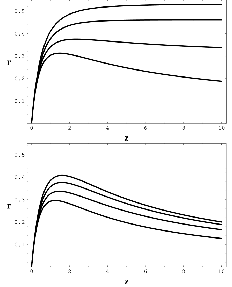
FIG. 1.: Top panel: DR distance for an empty beam ($\alpha=0$) with $\Omega_{m}=0.3$ and, from top to bottom, $m=0,1,2,3$. Bottom panel: the same for a filled beam ($\alpha=1$). Notice that for $\alpha=0$ there is quite a larger dispersion among the distances.

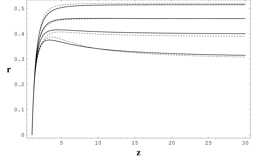
FIG. 2.: The solid lines are the numerical solutions for $\Omega_{m}=0.3$ and, from top to bottom, for $m=0.3;1;1.5;2.$ The dashed lines are our fits.

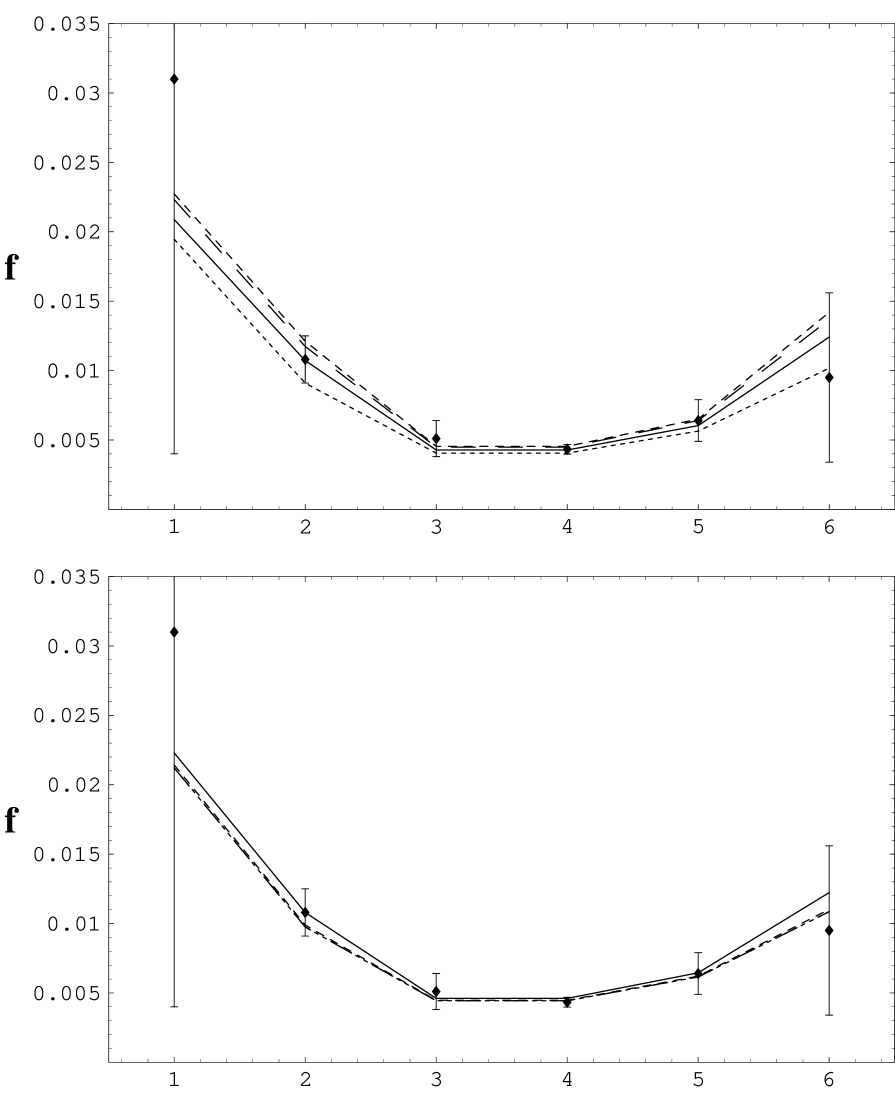
FIG. 3.: Top panel: comparison of the measured time delays $f$ of Table II (points with error bars) with the theoretical time delays (lines) for an empty beam and $H_{0}=71$ km/s/Mpc. The theoretical parameters are: $\Omega_{m}=0.1$  and $m=0$ (solid line) and $m=3$ (dotted line); $\Omega_{m}=0.9$ and $m=0$ (short-dashed line) and $m=3$ (long-dashed line). Bottom panel: the same as above but for a filled beam and $H_{0}=64$ km/s/Mpc.

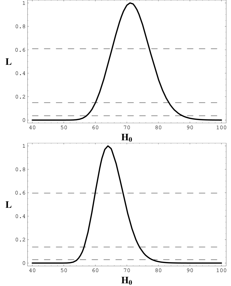
FIG. 4.: Top panel: The marginalized likelihood $L(H_{0})$ for $\alpha=0.$ The dashed lines mark the 1$\sigma,$2$\sigma$ and 3$\sigma$ levels. Bottom panel: Same as above but for $\alpha=1.$

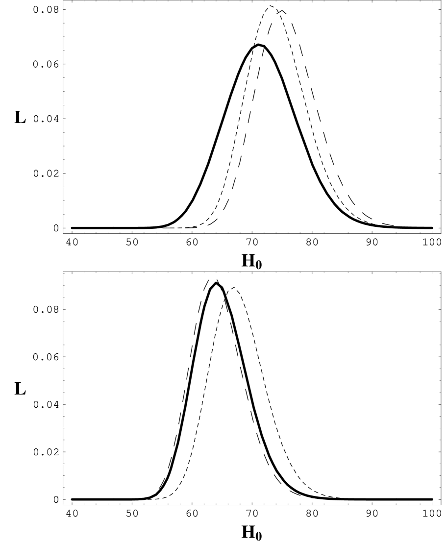
FIG. 5.: Top panel: comparison of the fully marginalized likelihood $L(H_{0})$ (solid line) for $\alpha=0$ with the likelihood obtained fixing the cosmology to two standard cases: pure cosmological constant ( $\Omega_{m}=0.3$ , $m=0,$ short-dashed line) and no quintessence ($\Omega_{m}=1$ , $m=3,$ long-dashed line). Notice the significant shift. Bottom panel: same as above but for $\alpha=1.$ Here the shift is reduced.

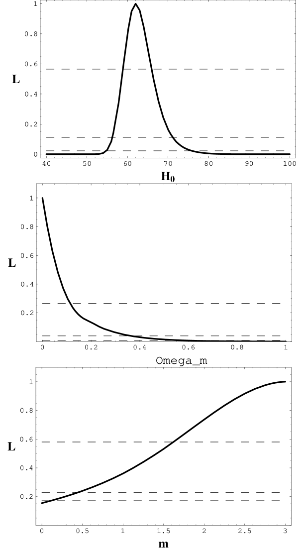
FIG. 6.: Simulation with a 10% error on time delays assuming $\alpha=0$. Top panel: marginalized likelihood of $H_{0}$ . The dashed lines are the levels at 1$\sigma$,2$\sigma$ and 3$\sigma.$ Central panel: marginalized likelihood of $\Omega_{m}$ . Bottom panel: marginalized likelihood of $m$ .