Microslit Nod-shuffle Spectroscopy — a technique for achieving very high densities of spectra

Abstract

We describe a new approach to obtaining very high surface densities of optical spectra in astronomical observations with extremely accurate subtraction of night sky emission. The observing technique requires that the telescope is nodded rapidly between targets and adjacent sky positions; object and sky spectra are recorded on adjacent regions of a low-noise CCD through charge shuffling. This permits the use of extremely high densities of small slit apertures (‘microslits’) since an extended slit is not required for sky interpolation. The overall multi-object advantage of this technique is as large as 2.9$\times$ that of conventional multi-slit observing for an instrument configuration which has an underfilled CCD detector and is always $>1.5$ for high target densities. The ‘nod-shuffle’ technique has been practically implemented at the Anglo-Australian Telescope as the “LDSS++ project” and achieves sky-subtraction accuracies as good as 0.04%, with even better performance possible. This is a factor of ten better than is routinely achieved with long-slits. LDSS++ has been used in various observational modes, which we describe, and for a wide variety of astronomical projects. The nod-shuffle approach should be of great benefit to most spectroscopic (e.g., long-slit, fiber, integral field) methods and would allow much deeper spectroscopy on very large telescopes (10m or greater) than is currently possible. Finally we discuss the prospects of using nod-shuffle to pursue extremely long spectroscopic exposures (many days) and of mimicking nod-shuffle observations with infrared arrays.

Accepted for publication in PASP

1 Introduction

The problem of subtracting the night sky foreground emission is a critical one for astronomical spectroscopy. The task is particularly acute in the red part of the spectrum (600$-$1000nm) as there are numerous hydroxyl (OH) bands which dominate the light giving a bright background. Many authors have recognized over the past twenty years that low to moderate resolution spectroscopy in this band is ultimately limited by systematic uncertainty associated with sky subtraction (e.g., Dressler 1984).

In some respects, it is surprising that optical astronomy has been slow to recognize an important technique utilized by near-infrared astronomy, i.e., beam-switching. Here, the background signal is very strong, is highly variable, and influences all observations (e.g., Ramsay,  et al., 1992). A common implementation of beam-switching is where the secondary mirror ‘chops’ between a target object and a sky field while the infrared array is read out continually.

This is perhaps because there is a conflict between the desire to beam-switch rapidly, and sample the sky contemporaenously, and the desire to take long integrations to minimize the effect of readout noise. This is especially true for modern, very low noise CCD detectors.

The underlying principle of the nod-shuffle technique is simply that a CCD detector can be used to store two images of a field, imaged quasi-simultaneously (Cuillandre et al. 1994; Bland-Hawthorn 1994; Sembach & Tonry 1996). By using ‘charge-shuffling’ charge can be moved from an illuminated region to a storage region. This process does not invoke readout noise and only takes only a fraction of a second since charge can be shifted between CCD rows two to three orders of magnitude faster than it can be read out. If this shuffling is synchronized to telescope motion two interleaved exposures of object and sky can be imaged side by side at the detector. Note three important facts: (i) the images are obtained through identical optical paths, (ii) the imposed flatfield structure is identical for both images, and (iii) the CCD is read out only once.

The use of shuffling techniques in astronomy can be traced to early attempts to improve the performance of imaging polarimeters (McLean et al. 1981; Stockman 1982). Since that time, charge-shuffling has been little utilised. Part of the reason may stem from experiments by Lemonier & Piaget (1983). By rapidly shifting charge backwards and forwards many times (pocket pumping), they were able to identify local defects in the potential profile (trapping sites) within the silicon substrate. By the end of the 1980s, traps and deferred charge were still a fundamental limitation to repeated charge shuffle operations (Blouke et al. 1988).

The development of charge-shuffling at the Anglo-Australian Observatory dates back to the 1994 Marseilles conference on imaging spectrographs (Comte & Marcelin 1995). It was here that the first results of integral field spectrographs were presented, arguably the most important development in optical instrumentation in the past decade. It was clear, and remains true, that the fundamental limitation of this powerful technology is the difficulty of accurate sky subtraction (Bland-Hawthorn 1995).

Key developments in CCD manufacture have made charge-shuffling a realistic prospect and an important consideration in all future instrument design. First, the latest generation CCDs (EEV, MIT Lincoln Lab) have very low read noise ($\sim 1e^{-}$), negligible dark current, high purity and very high charge transfer efficiency (99.9999%). Secondly, the manufacturing process prefers to generate rectangular arrays which provide for storage regions. Bland-Hawthorn & Barton (1995) demonstrate that, with modern CCDs, it takes more than a hundred shuffle operations before bulk trapping sites start to compromise the data.

In this paper, we describe the development at the AAO of the ‘nod-shuffle’ method founded on the principle of CCD charge shuffling. This differential technique has resulted in two important experimental breakthroughs. First, the object and sky can be measured quasi-simultaneously. As we show, the main limit to the accuracy of sky-subtraction is the rapidity of nod-shuffling compared to the temporal power spectrum of sky brightness variations. Secondly, nod-shuffle allows for a considerable increase in the multi-object gain of a spectrograph, up to 2.9$\times$ more objects per unit observing time using small ‘microslits,’ for fields with high object densities. We have implemented the nod-shuffle method with the Low Dispersion Survey Spectrograph (LDSS) on the Anglo-Australian Telescope (AAT) and have obtained fractional residuals as low as $4\times 10^{-4}$.

The plan of this paper is as follows: in Section 2 we describe the nod-shuffle concept and discuss qualitatively the sky-subtraction and multiplex advantages to be gained. In Section 3 we describe in detail our implementation of nod-shuffle at the AAT using the Low Dispersion Survey Spectrograph and show some example data. In Section 4, we show the increased multi-object gain which becomes possible via the nod-shuffle operation. We quantify the sky-subtraction accuracy in Section 5 and discuss ways in which it might be improved further. In Section 6, we illustrate key observing modes for LDSS++ which are facilitated by the use of microslits. Finally, we discuss future prospects for the nod-shuffle observing mode.

2 The Nod-Shuffle Concept

The concept behind charge shuffling is that unilluminated portions of a CCD can be used for storage. The image formed on an illuminated portion can be ‘shuffled’ very quickly into a storage area by clocking before being shuffled back at a later stage. For example, with the AAO-1 CCD controller and the Thompson 1024$\times$1024 format CCD, a single row can be shifted upwards or downwards in 12.5 $\mu$s, compared to 30–160 ms when clocked through the output amplifiers. The shift operation is a factor of 4 slower for the Tek 1024$\times$1024 format and MITLL 2048$\times$4096 format CCDs. Since the shuffle operation does not involve the read-out amplifiers, the primary source of noise is now associated with charge transfer within the substrate (Janesick & Elliott 1992).

Each vertical clock shifts the complete image on the CCD one row up towards the readout register. The row that was next to the readout register gets clocked in to the readout register and cannot be reverse clocked back into the image. At the other end of the image, a ‘clean’ row is generated. This happens for shifting in the ‘forward’ direction. Clocking in the reverse direction moves the complete image one row away from the readout register for every vertical clock applied to the CCD. A clean row is generated next to the readout register and at the other end one image row is lost.

In order to produce two contiguous images side by side on the detector via shuffling, the maximum field of view (i.e., number of rows) which can be shifted without loss of information for the exposed or stored image is one third of the detector’s column dimension. The reason is clear: when the detector is clocked in one direction, rows at the detector edge are lost (c.f. Figure 1). More generally, shuffling between $m$ partitions uses $m/(2m-1)$ of the CCD for holding the separate observations, while the remainder is (a) used for temporary storage, and (b) rendered useless by the shuffle process (i.e., this fraction is never illuminated). A fuller technical description of charge-shuffling is given in Bland-Hawthorn  et al. (2000).

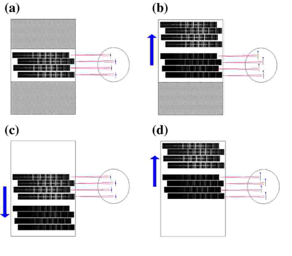
Figure 1: Illustration of the nod-shuffle procedure implemented in the LDSS spectrograph showing progressive stages of image formation: (a) The spectra of the objects through the slits is imaged onto the central portion of an oversized CCD. (b) The first image is shuffled up into a storage region (with the shutter closed), the telescope is offset to adjacent sky which is then imaged onto the now empty central region of the detector. (c) The object image is shuffled back and additional object photons are imaged (d) Sky is shuffled back and imaged. Steps (c) and (d) are cycled continuously until the integration is complete.

The nod-shuffle image sequence developed for LDSS observing is utilises this underfilled, large-shuffle mode and is illustrated in Figure 1. The observing sequence is as follows:

1. The target objects are acquired with the telescope on to the spectrograph mask slits (these may be true slits or simple apertures such as holes).

2. The shutter is opened for a OBJECT exposure (usually 10–100 secs in duration), dispersed spectra of OBJECTS$+$SKY are accumulated in the central area.

3. The shutter is closed.

4. The OBJECT image is shuffled up, by clocking the CCD charge pattern. to a upper storage area which is unilluminated.

5. The telescope is moved to a SKY position. (This can be a truly blank patch or can simply involve moving the objects some way along the slits).

6. The shutter is re-opened and dispersed SKY spectra are accumulated, for the same exposure time as the OBJECT, in the blank central area.

7. The shutter is closed, the charge is shuffled back down bring the OBJECT image back in to the center and the SKY image into blank storage. The telescope is moved back to the OBJECT position.

8. The shutter is opened and more OBJECT data is accumulated.

9. The sequence OBJECT–SKY–OBJECT–SKY–… is repeated for the rest of the exposure.

At the AAT, the OBJECT and SKY exposures are typically 30 secs, repeated to fill up a 1800 sec exposure before readout. Sky subtraction then consists of extracting the two regions and calculating the difference image. This technique, which we call “nod-shuffle,” gives extremely precise sky-subtraction for the following reasons:

a

The OBJECT and SKY are observed through identical slits/apertures. The effect of any irregularities cancel out in the subtraction.

b

The OBJECT and SKY are imaged on to the exactly the same pixels on the detector. The optical path is identical. The pixel response is identical. (The response is that of the pixel where the image is measured — the storage pixels have no effect).

c

The OBJECT and SKY are observed quasi-simultaneously, thus the effect short timescale temporal sky variations cancel out in the subtraction. This is quantified below in Section 5.

d

The OBJECT and SKY positions can be extremely close (a few arcsecs) so spatial sky variations are not significant.

e

Because of the identical light path and quasi-simultaneity the effects of fringeing on the detector from night sky lines cancels out.

f

Similarly the effects of any instrument flexure during the course of the exposure cancel out.

g

There is no need to re-sample and interpolate the sky for the subtraction, so there are no numerical artifacts introduced.

h

The presence of any DC level in the detector due to bias, dark current, or scattered light does not affect the sky-subtraction. If it is constant it cancels, if it varies across the detector (including the unilluminated regions) it will not cancel but will still not affect the sky subtraction.

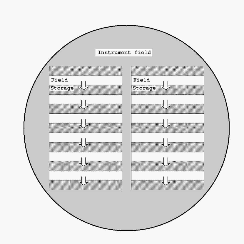
Figure 2: Illustration of the nod-shuffle geometry in the case in which the detectors are overfilled by the instrument field of view (FOV) (in this case two detectors are shown). Unilluminated regions must be taken from the active FOV giving a 50% overhead resulting in a stripe pattern. Note the stripe width can be as small as individual spectra, however it is desirable to make them larger to minimise area lost to edge effects at the strip boundaries: a region of wide $\simeq$ instrument PSF will be badly subtracted. A reasonable width would be large banks 20–50 spectra.

Of course this is a much more complex observing sequence than simply acquiring objects on to slits and staring. There is also a penalty for the precise sky-subtraction: $\sqrt{2}$ more noise in the resulting spectra because of the subtraction, compared to a very long slit, though the systematics in the sky removal are expected to be greatly improved.

However nod-shuffle offers another great advantage over conventional multislit spectroscopy: it permits a large increase in the achievable object multiplex. Because a long slit is no longer required for sky-subtraction via interpolation the apertures only need be large enough to cover the objects. We term these “microslits”. Additionally they need not be slits — they can be apertures of any shape such as circles. If we take the example of observing faint 24^th magnitude galaxies only a 1 arcsec aperture is required due to their small size (Smail et al. 1995). Comparing this to typical multislit observations with 10–15 arcsec long slits (Glazebrook et al. 1995), we can see that we would expect 10–15$\times$ as many slits to be squeezed on to the mask without spectral overlap. We quantify these multiplex gains below in Section 4.

Finally we note that for multi-object spectroscopy there is an alternative mode of observing where the charge is shuffled only a few pixels. Because a slit mask blocks out light any part of the CCD can be used for storage. This is particularly useful because it scales to multiple, mosaicked CCDs i.e. when the camera FOV is much bigger than the detectors. This case is illustrated in Figure 2. A penalty here is that half the available detector area must be used for storage when it could be used on-sky, however as we demonstrate below it still gives a formal multiplex advantage in the high source density limit.

3 The AAT/LDSS++ Implementation

The practical implementation we will describe was developed using the AAT’s Low Dispersion Survey Spectrograph (LDSS), which came to be known as the LDSS++ project. LDSS is a wide-field multislit spectrograph with a 12 arcmin field of view. A large collimator re-images the telescope pupil, in this space can be inserted grisms and/or filters, this is then imaged through a camera onto a CCD detector (Wynne & Worswick 1988; Glazebrook 2000). The grism can be taken out for direct imaging of the field or the mask, this is used to acquire the field on to the mask accurately.

LDSS has recently been equipped with a volume-phase holographic grating (VPH; Barden, Arns & Colburn 1998) and a MITLL deep-depletion $2048\times 4096$ CCD detector with 15$\mu\rm m$ pixels. These two upgrades give a considerable improvement in the red 500–1000nm throughput of the system: the gain at 700nm is a factor of 2 (Glazebrook 1998).

The LDSS field of view is circular and is $\simeq 2000$ pixels on the detector (0.39 arcsec pix^-1 scale). The shuffle direction is along the long axis of the CCD, perpendicular to the dispersion direction exactly as shown in Figure 1. This is not absolutely necessary but is done because it is easier to block the adjacent storage areas spatially by using the mask; otherwise some sort of spectral blocker would be required and this would not be ideal due to offsets between slits. In nod-shuffle mode we thus use the central $2048\times 1365$ pixels. It represents approximately the underfilled case described in Section 2.

The implementation of our nod-shuffle scheme is as follows. At the start of a nod-shuffle run, a shuffle sequence is downloaded to the CCD controller micro and the instrument sequencer micro from the VAX computer; the instrument sequencer also receives a telescope command set. The VAX then tells the instrument sequencer and the CCD controller to ‘run’. The controller runs software which interprets the shuffle sequence, clocking the charge up and down and driving the CCD shutter. It dictates each step by triggering an event with an ‘external sync’ pulse for each phase of the operation. The triggers occur after fixed time intervals since there is presently no handshake from the telescope. The number and nature of the triggers depend on whether there is to be guiding at either the object or sky position (OFFSET mode), at neither (OFFSET NO GUIDE mode) or both (AXES mode). With the output pulse, the CCD controller toggles the status of an I/O line and waits for a given delay time. The instrument sequencer reads the I/O line and, when required, writes telescope control commands to a port on the VAX/VMS computer system. A program running on the VAX reads these commands, translates them and routes them via the CAMAC interface to the telescope control Interdata computer.

There is no feedback in this system: the CCD controller does not know the state of the telescope. Ideally of course it would, but this would require complete re-engineering of the whole observing system. Instead the telescope movement is allowed for by predetermined time delays. The controller waits a given amount of time between shuffles with the shutter closed to allow the telescope to finish its ‘offset and stabilise’ action. For small offsets of a few arcsec, the AAT does this in about 1 second; typically we allow 2 secs dead time in a 30 sec integration time. It was verified that this was adequate by taking long-exposure direct images of star fields in nod-shuffle mode and looking for image elongation along the offset direction. The two shuffled images can also be subtracted to look for elongated residuals — none were found down to the noise level.

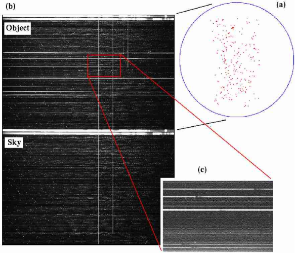
Figure 3: Sample data from the HDF-S observing campaign. Panel (a) shows the slitmask used (225 microslits) and panel (b) shows the raw shuffled data. (c) shows the difference image zoom,ed in. The slits in the case are circular apertures, so the spectra appears as tramlines a few pixels wide horizontally across the detector. Panel (d) shows two sample extracted spectra of a bright and faint galaxy, the solid lines are the spectra (unfluxed) and the lower dotted lines show the theorectically achievable noise level as determined by shot and read noise (shot dominates). Bad columns are masked out of the plot. Sky residuals are only seen near extremely bright lines (5577Å and 6300Å are marked as examples) and are entirely consistent with pure Poisson variance.

Some sample data of nod-shuffle spectra are shown in Figure 3. This was taken for a redshift campaign in the Hubble Deep Field South (Glazebrook et al. 2000a) during commissioning of the nod-shuffle system. We placed 225 microslits (circular $\simeq 1$ arcsec apertures) on targets along the 1365 pixel spatial axis ($\equiv$ 9 arcmin), the spectra are dispersed along the horizontal 2048 pixel axis ($\equiv 5300$Å). The LDSS PSF is a Gaussian with 2 pixels FWHM at the field field degrading to 3 pixels at the field edge. The microslits are spaced at intervals of at least 4 pixels vertically (subject to target availability) so their spectra are significantly separated. The horizontal spread of the slits was up to 3 arcmin so as not to introduce significant wavelength offsets between spectra.

It can be seen in Figure 3 that the form of this data is somewhat akin to spectra from fiber optic spectrographs in that each object produces a tramline which is traced and extracted. However in this case the extraction is done after sky-subtraction and there are significant wavelength offsets between spectra.

4 Multiplex gains

To quantify the multiplex gain we must compare the number of spectra observable per unit time to the same limiting signal$/$noise ratio versus the longslit case where the sky is subtracted by interpolation. We must observe for longer with nod-shuffling to reach the same signal$/$noise, however this is more than balanced by an increase in the number of slits we can fit on the mask. We call this the ‘nod-shuffle advantage’ (NSA).

The OBJECT$-$SKY subtraction in the nod-shuffle case introduces $\sqrt{2}$ extra subtraction noise. First we consider at what length the longslit subtraction introduces the same amount. We will assume the longslit has length $n$ elements, where an element is taken as the spatial extent of the target objects (thus $n=1$ for the microslit).

Conventionally the background along the slit, excluding the object, is fitted with either a linear model or a higher-order polynomial. Typically the background level will vary by a few percent across the slit due to instrumental effects such as slit alignment and optical distortion and this slope will vary with wavelength due to the structure in the sky spectrum. The fitting will also be limited by the presence of slit irregularities. This is discussed in more detail below in Section 5. For now we will compute the ideal limit for a smooth slit.

Accurate sky-subtraction in the neighbourhood of the bright sky emission lines requires fitting at least a general linear model to each wavelength channel, thus the error at the object location is the error on the intercept on the slope ($\sigma_{c}^{2}$) from the line fitting from $N$ points:

$$\sigma_{c}^{2}={2\sigma^{2}(2n+1)\over n(n-1)}\simeq{4\sigma^{2}\over n}\ \ \ (n\rightarrow\infty)$$

where $\sigma$ is the noise on each point and for simplicity we have ignored the omission of the central object point. We now consider the following question: as the slit length $n$ increases at what point does subtracting the linear fit introduce less noise than nod-shuffling, i.e. $\sigma^{2}+\sigma_{c}^{2}<2\sigma^{2}$?

This occurs at $n=6$, after allowing for more complex formulae where the central point is omitted. Instead of the slit we could in principle substitute 6 microslits. There is a factor of two nod-shuffling overhead either temporally (due to the sky position) or spatially (if we move the object between adjacent slit positions we have 3 pairs rather than 6 objects). For $n=6$ we calculate $\sigma_{c}^{2}=0.95\sigma^{2}$ and so the NSA is calculated to be 2.9. As slits become longer the NSA increases further and tends to $n/4$ for large $n$. While we can fit on $n\times$ more slits we have to observe $4\times$ longer to allow for the two positions overhead and subtraction noise.

In practice, as the slit becomes longer more instrumental effects come into play and a linear fit no longer improves the residuals. Often a higher-order polynomial is used to allow for curvature, however this will introduce yet more noise as there are more free parameters. In practice a slit length of 15–20 arcsec is the useful limit, if slits are this large the NSA is 4–5.

For the overfilled case illustrated in Figure 2 there is another additional factor of two for charge storage in regions which could otherwise be used for observations; nevertheless the NSA is still 1.5 exceeding the longslit case and providing better sky-subtraction.

Of course the theoretical NSA is only achieved if the object density is high enough to allow close spacing of microslits. In the very low density regime where a very long slit can be placed on each object with no concomittant multiplex loss the NSA is only 0.5, i.e. we must observe twice as long to balance the $\sqrt{2}$ subtraction noise. In practice however for faint spectroscopy typical slit spectroscopy is dominated by residual systematics at the 0.5–1% level (see Section 5) and not random noise where the lines are bright. And at low resolutions ($R<2000$) a large fraction ($\sim 50\%$) of the red spectrum is occluded by bright lines, so the supposed $S/N$ loss is moot.

One common technique to reduce these sky residuals in otherwise conventional longslit observing is to use a ‘slow’ beam-switching technique to improve the systematic residuals when observing ultra-faint targets by moving the object along the slit in consecutive observations. This is analogous to nod-shuffle except the CCD is read out between the two positions. The individual exposures must be at least 5–10 minutes (on a 4m telescope) to obtain enough sky signal to be background limited and consequently when the images are subtracted there is a residual due to temporal sky changes. This residual is removed again by fitting along the slit, but the systematics are reduced because of the lower overall level. Like nod-shuffle this will always introduce $\sqrt{2}$ more subtraction noise. The minimum NSA versus this case is now 5.9 (underfilled) and 2.9 (overfilled).

So far we have made the assumption that an independent linear fit must be done for each wavelength. However if the sky background has no structure, i.e. is observed in a wavelength region of featureless continuum, then we would expect the slope across the slit to vary only slowly with wavelength and the fitting can in principle be highly constrained. The underfilled NSA reaches 0.5 in this limit. However even in the blue part of the optical spectrum (350–500nm) there is still considerable stucture in the night sky spectrum due to scattered solar absorption lines.

Finally the NSA is maximised at very high target densities. The required density is approximately:

$$\rho={3600\beta\over W\alpha\,x}\ \ \ \hbox{objects\ arcmin}^{-2}$$

where $\beta$ is the dispersion in Å$/$pixel, $\alpha$ is the spatial scale in arcsec$/$pixel, $x$ is the microslit size in arcsec and $W$ (in Å) is either the wavelength range on the detector (when the spectra are short compared to the detector size) or the minimum wavelength overlap required for all objects by the mask design (when the spectra are comparable to or longer than the detector). For LDSS++, $\alpha=0.39$ arcsec pix^-1, $\beta=2.6$ Å pix^-1, for the HDF-S project we used $W=3000$ Åand $1.0$ arcsec apertures. This gives a sky density requirement of $\simeq 8$ objects arcmin^-2. For field galaxies this density is achieved at $R\approx 23$ (Hogg et al. 1997; Smail  et al. 1995). It is also very suitable for observing stellar and galaxy clusters. It is a much higher density than can be achieved by conventional multislits ($\sim 5$–$10\times$) and by fiber spectrographs — for example the highly multiplexed 2dF spectrograph can only reach 0.05–0.1 objects arcmin^-2 (Lewis et al. 2000).

5 Sky subtraction accuracy

5.1 Achievable accuracy with conventional multi-slits

In order for the figures for nod-shuffle accuracy to be meaningful, it is useful to consider how well sky can be subtracted using a longslit. This is limited by instrumental imperfections such as variable PSF, slit and CCD irregularities, slit tilt and pixel sampling effects, image distortion, fringeing, flexure etc. The effect of slit tilt, with respect to the CCD columns, is particularly intresting as it is this which causes linear sky variations across the slit. If we consider the tilt as an angle $\theta$ then we expect fractional sky variations along the slit:

$${\Delta S\over S}={1\over S}{\partial S\over\partial x}L\sin\theta$$

where $L$ is the distance along the slit in pixels and ${\partial S/\partial x}$ is the rate of change of the sky count $S$ with pixel $x$ in the spectrum. The instrument is usually critically sampled so the PSF is 2–3 pixels. This means we expect fractional sky fluctuations of order unity between spectrally adjacent pixels in regions near bright sky lines. This gives:

$${1\over S}{\partial S\over\partial x}\simeq 1$$

In the LDSS case the achievable rectilinear alignment is 1 pixel in 1000 giving $\theta=0.05^{\circ}$. In our experience this is typical of modern spectrographs as mechanical tolerances are usually designed so that alignment is possible to $\sim$ a CCD pixel. Image distortion in the optics also turns out to be a big effect. LDSS is a typical fast $f/2$ camera. The change in radial distortion across a slit length will introduce an apparent rotation ($\theta^{\prime}$) if the slit is off the cardinal axes. A useful formula for this is:

$$\theta^{\prime}={\partial D\over\partial r}{xy\over r^{2}}$$

for a slit at $(x,y$) wrt the optical axis axis (radius $r=\sqrt{x^{2}+y^{2}}$) where the radial distortion $D=r_{2}-r_{1}$.

In the LDSS optics the typical distortion $\partial D/\partial r\simeq 0.02$, thus we can estimate typical apparent rotations (using $x\sim y\sim r$) of $\theta^{\prime}\sim 2^{\circ}$. Many similar systems have fast cameras (e.g. the LRIS Keck multislit spectrograph camera is $f/1.56$ and using the LRIS astrometry software we find distortions of $\sim 10$ pixels over 400 pixels, so $\partial D/\partial r\simeq 0.02$ ) so we expect this order of radial distortion to be typical of modern fast spectrographs.

Putting these formulas together this rotation would cause a linear sky gradient of order 30% across a 10 arcsec slit. If the data could be resampled to sub-pixel accuracy to correct for tilts, we could expect to achieve 0.1 pixel accuracy which would still leave 10% variations.

In principle though smooth variations can be removed. However another effect is slit irregularities. The milled metal slit masks used in LDSS have 10–20 $\mu\rm m$ irregularities (1 arcsec = 150 $\mu\rm m$ at AAT’s $f/8$). This is typical of machine cut masks (Szeto  et al., 1996). Thus we also expect $\simeq$ 10% semi-random variations along the slit due to this effect. This can be flatfielded out by dividing by a dispersed white light exposure, this will be limited by flexure between the white light and the data exposure. LDSS flexes at about 0.5 pixels$/$hour thus we can expect a misalignment of order 0.1–0.2 pixels giving residuals of order 1%.

So we are in a situation in LDSS where we are fitting slopes of order 10–30% with a slit length of 10–20 pixels and with systematic variations of $\pm 1\%$. The sky lines in LDSS at low-resolution have peak counts of $\simeq 2000$ electrons in a half hour exposure, so the random noise will be about 2%. Fitting along the slit would reduce this to $\mathrel{\lower 2.58334pt\hbox{$\buildrel{\textstyle<}\over{\scriptstyle\sim}$}}1\%$ at which point it is comparable to the systematic slit irregularities.

How faint can we go with 1% sky-subtraction accuracy? In the $I$-band the sky background is dominated by the lines, if we demand an object has $S/N\sim 3$ then the faintest that can be reliably reached, in any exposure time, is $I_{AB}=23.6$ per arcsec². Fainter than that the fluctuations in the spectrum will be dominated by sky residuals at the lines, and for low-resolution $I$-band spectroscopy the lines occlude most of the spectrum.

How could this be improved? One crucial area with scope for improvement is the microroughness of the slit edges.

5.2 Improving multi-slit accuracy

Conventional laser cutting (melting and vaporization) of metal (e.g., Al) masks produces 10$-$20$\mu\rm m$ roughness. During manufacture, most metals undergo warping during cutting which defocusses the laser. This is one of the major sources of error in slit manufacture which in turn contributes to poor sky subtraction.

Recently, new slit masks made with laser-cut carbon fiber have already achieved an order of magnitude improvement in edge roughness (Szeto et al. 1996). An important step by the Gemini/GMOS team (Stilburn, private communication) was to use epoxy-bonded sheets made of 3-ply unidirectional carbon fiber with a total thickness of only 200$\mu\rm m$. The center ply is orthogonal to the outer plies, and the slits are cut at 45^∘ to the fiber direction. The low-power Nd:YAG laser cuts slits at 10 mm s^-1 and, remarkably, achieves a 1$-$2$\mu\rm m$ edge roughness.

Let us assume an 8m size telescope with a larger image scale. At $f/16$ a 1 arcsec slit would be 600 $\mu\rm m$ so the irregularities would be 0.1–0.2%. The larger mirror will accumulate more light, so we would reach this limit in a 3 hour exposure, faster if our spectrograph was more efficient. At 0.1% of sky we are now observing at a surface brightness limit of $I_{AB}=26.1$ per arcsec² with forseeable multi-slit technology. Improving the instrumental resolution will reduce the amount of spectrum occluded by sky lines, though the peak counts in the lines will stay approximately the same as they will stay unresolved. There will be a danger of running into detector dark and readout noise limits.

5.3 Nod-shuffle sky-subtraction accuracy

It is clear that the acheivable accuracy of sky-subtraction with the nod-shuffle technique depends on how rapidly the nod-shuffling is done. If this is done at a fast rate changes in the night-sky background are sampled more accurately, as well as changes in the instrument such as flexure. However characteristic timescales for the latter are of the order of hours, so sky temporal variations will be the limiting factor on the residuals.

In order to empirically measure the accuracy of sky-subtraction we used a sequence of 8 longslit spectra, collected on 2–3 April 2000 at the AAT in longslit mode. The targets were faint QSOs ($I\leq 22$) in a scheduled AAT science project, by arrangement with the observers the observations were done so as to allow us to try out different nod-shuffle times. The slit wss 4 arcmin long and the longslit data were collected in nod-shuffle mode with the targets nodded 5–10 arcseconds along the slit. The log of the observations is given in Table 1. A sample raw data frame is shown in Figure 4.

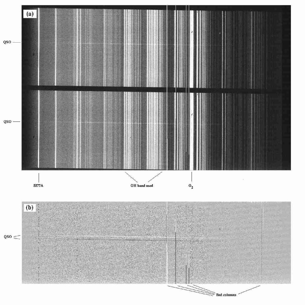
Figure 4: Example of the longslit data which goes into our sky-residual analysis. (a) Raw, shuffled image (except for cosmic rays being patched out). (b) A-B subtracted image showing the 2D residuals. Residuals are integrated along the slit and across a wavelength range as described in the text.

Table 1: Log of observations for the nod-shuffle sky residual analysis, all 1800s total integration time

AAT RUN	NS-Time/secs	UT start	Remarks
02APR0001	30	09:46:54	Some cloud (5/8ths)
02APR0008	15	13:06:03	${}^{\prime}\,{}^{\prime}$
02APR0010	7.5	14:00:32	Clear
02APR0012	30	15:18:48	${}^{\prime}\,{}^{\prime}$
03APR0004	60	14:17:06	Clear, bad seeing (5–$10^{\prime\prime}$)
03APR0005	60	14:50:51	${}^{\prime}\,{}^{\prime}$
03APR0007	30	15:40:35	${}^{\prime}\,{}^{\prime}$
03APR0008	30	16:15:11	${}^{\prime}\,{}^{\prime}$
05APR0007	300	14:29:03	Clear, v. bright O2 emission (8645Å)
06APR0004	150	09:25:45	Clear, seeing 2–2.5′′
06APR0005	450	09:58:54	${}^{\prime}\,{}^{\prime}$

All the frames had the same total exposure time of 1800s, the only change was the rate of nod-shuffling which we varied from as fast as 15s to as slow as 450s. Once the QSOs are masked out the sky region of the 2D images can be used to quantify the effect of the nod-shuffle time on sky residuals. The data processing sequence is extremely simple:

1. Frames are bias-level subtracted.

2. A median-filter smoothed version of each frame is made. The smoothing is entirely along the spatial (Y) axis with a smoothing kernel of 21 pixels (8.2 arcsecs). Because the slit is very closely aligned with the CCD columns ($\leq 1$ pixel) and the CCD has good flat-field characteristics this essentially replaces each pixel with a smoothed estimate robust against cosmic-rays.

3. The smoothed frame is used to calculate the variance map of the raw frame assuming shot noise from the sky and the know readout noise of the detector.

4. Cosmic rays are identified as $>10\sigma$ peaks in the RAW$-$SMOOTHED map and used to calculate an exclusion mask. Any pixel within 5 pixels of a cosmic ray peak are masked. Cosmic ray identifications are checked visually. This mask excludes about 1% of all pixels on each frame.

5. The cosmic ray mask is ORed with another mask which excludes several bad columns and the centre rows where the QSO spectra lie.

6. A sky spectrum is formed for each frame by averaging unmasked pixels along the slit. A variance spectrum is also calculated.

7. A residual sky spectrum is formed for each frame by repeating step 6 for the residual A$-$B frame.

To calculate the fractional sky-residual $\Delta\hbox{sky}/\hbox{sky}$ we can integrate the residual and sky spectra in wavelength and divide. Absolute flux calibration is not necessary. We chose two wavelength regions: the first region encompasses the two main OH regions in the $I$-band (7200–8880Å) and the second region encompasses the 5577Å OI line (60Å width bandpass). We choose to fit and remove the continuum level from the spectrum before doing the summation. This is because there is not enough unilluminated space on the detector to allow accurate determination and extrapolation of the level of scattered light. In any case the integrated sky-brightness is dominated by the lines, not the continuum, and it is the temporal variation of the line flux we are primarily concerned with. Since our sky-spectrum is also integrated along 4 arcmins of slit we can go very deep in measuring systematic residuals.

Figure 5: Sky residuals in a 1800s exposure as a function of nod-shuffle time. The upper line in each panel show the raw sky$/10$, the lower points (with error bars) show the residual after nod-shuffle subtraction. A clear point-point systematic is seen in the 300s nod-shuffle exposure, while the others are consistent with zero.

Our results are shown in several figures. Firstly Figure 5 shows raw and residual spectra for our two regions for different nod-shuffle times. Figure 6 shows $\Delta\hbox{sky}/\hbox{sky}$ plotted against nod-shuffle time for the two regions. There is a clear trend of systematics consistent with scatter around zero at the level of $\pm 10^{-3}$ for small nod-shuffle times ($<$100s), the level of the scatter is about 3$\sigma$. For large nod-shuffle times $>$100s there are gross systematic residuals at the $\pm 10^{-2}$ level.

One limitation of our particular nod-shuffle technique is we observe an asymmetric seqeuence:

$$ABAB...ABAB$$

If there was a systematic change in sky-brightness during the course of the observations we would expect to see a residual because the average $B$ frame is slightly later in time than the average $A$ frame. A systematic decrease in OH emission during the course of the night is often observed (Leinert  et al. 1998). This effect is normally explained as the result of energy stored during the day in the respective atmospheric layers (Kondratyev 1969). We see evidence for exactly this effect, with the correct sign, in our data (Figure 7). An additional source of long-term variation is the effect of changing airmass during an extended observing sequence on a single source (Bland-Hawthorn et al. 1998). In principle it is straight-forward to reduce these effects by improving the nod-shuffle method with a symmetric mode, i.e.:

$${B\over 2}ABA...ABA{B\over 2}$$

Then the $A-B$ subtraction would cancel out any linear trend. However we have yet to try this in our AAT implementation.

The effect of drift should also cancel to some extent for long all-night nod-shuffle exposures which bracket local midnight. It would be desirable to take much longer integrations with a fast nod-shuffle rate to explore the limits of this technique. While we do not have this data as such, what we can do is stack all our data where the nod-shuffle time is $<$100s. This gives us a 5.5 hour very deep exposure, albeit with a variable nod-shuffle time. The residual point from the 5.5 hour stack is $(4.0\pm 1.2)\times 10^{-4}$ — a $3\sigma$ detection. It is important to realise that this is an impressively small residual corresponding to a $I_{AB}=28.3$ mags arcsec^-2 source. This level of accuracy is a factor of 10–20$\times$ better than is typically achieved with slits (see Section 5.1).

Figure 6: Sky residuals vs nod-shuffle time for the chosen OH band and the 5577Å line. The rectangles indicate the range of the +/- 1$\sigma$ errors vertically and are filled for OH, open for 5577Å. Small artificial offsets temporal are used at 30s and 60s to show the multiple points with clarity.

Figure 7: OH sky residuals vs UT for nod-shuffle times $<$100s. Local midnight (14^hUT) and the end$/$start of twilight are indicated by dotted lines. We expect to see a negative residual at the start of the night and the residuals should have a positive slope with time, we do in fact see this.

We also emphasize that this is a lower limit to what could be achieved with faster nod-shuffle times. One could nod-shuffle faster (e.g. 10s) for a whole very long exposure. Also one should implment the symmetric mode to cancel long-term sky-brightness drifts. Finally for the ultimate sky-subtraction limits one could combine nod-shuffle with slits to allow for 2D interpolation and removal of any local residuals after nod-shuffle subtraction. Accuracies of $10^{-4}$ or better should be achievable.

5.4 Comparison of residuals to theorectical predictions

We have shown that the nod-shuffle residuals appear to be characteristically smaller for nod steps below 100 sec compared to longer sample exposures. We now examine this with a simulation of the nod-shuffle technique using a model which attempts to describe the time-variable behaviour of OH emission.

Suitable observations for deriving the temporal power spectrum of OH are hard to come by. Line strength variations on timescales of 5–10 mins are given by Bland-Hawthorn et al. (1998) for optical lines and Ramsay et al. (1992) for near-infrared lines. The latter reference shows the OH behavior to be approximately sinusoidal on timescales of an hour with a peak-to-peak amplitude of about 10%. On longer timescales, the OH variation is more erratic.

Our model for atmospheric variability uses a finite set of sinusoidal modes with periods 16, 23, 26, 29, 38, 51 and 101 mins. The amplitude of the variations are inversely related to the period such that the 16 min dominates, in rough accordance with the wave-like structures observed by Ramsay et al. (1992). The peak-to-peak amplitude is 15% of the mean line strength. For each mode, there is a 5% dispersion in the period and amplitude, each with random phases. Our predicted behavior is in good agreement with the above references.

Figure 8: Example OH airglow time series generated from our model. The shaded bands indicate periods of 400 secs.

However, high cadence observations show clear evidence for stochastic behavior on shorter observational timescales. Here, we found data from the 2MASS Wide-field Airglow Experiment to be the most useful (Adams & Skrutskie 1997). The H band observations have an order of magnitude finer sampling than in Ramsay et al. (1992). We simulate this by including a component of $1/f$ noise within our model (cf. Barnes & Allan 1966). To generate the $1/f$ component we use gaussian white noise scaled to 5% ($1\sigma$) of the mean line strength (see Adams & Skrutskie 1997, Fig. 2) convolved with Green’s impulse function ${\cal I}(t-t_{o})=c(t-t_{o})^{-0.5}$ ($t>t_{o}$); ${\cal I}(t-t_{o})=0$ ($t\leq t_{o}$) . For convenience, we set $c=1$ and sample the time axis in units of seconds. An example time series is shown in Figure 8.

Figure 9: Simulation of the expected residuals in a 1800s exposure for different nod-shuffle times. This should be compared with Figure 6.

In Figure 9, we have attempted to simulate nod-shuffle sampling of our model atmosphere. The total exposure time is 1800 secs and the time series is sampled at all possible time steps (longer than or equal to 10 sec) that lead to an integer number of cycles. For each nod exposure, the simulation was run 10 times. The mean residuals (and $1\sigma$ errors) are shown as a function of the nod exposure. There is a evidence for a change in character on either side of about 2 min time steps. The residuals with 2 min samples or longer are $10^{-3}$ or larger; the residuals from faster sampling are $1-4\times 10^{-4}$.

Repeated runs of our model atmosphere show that this changeover can be as short as 1 min. There are also times when short sample time steps lead to big residuals (e.g. 20 sec) and when long time steps lead to residuals smaller than $10^{-3}$. These are times when the nod-shuffle sequence happens to fall in or out of step with a beating atmosphere. Airglow is clearly a complicated phenomenon: empirically it is clear that the nod-shuffle time should be $\mathrel{\lower 2.58334pt\hbox{$\buildrel{\textstyle<}\over{\scriptstyle\sim}$}}30$ sec. The total number of shuffles should not greatly exceed $\approx 10^{2}$ per readout if one is to avoid significant degradation from trapping sites within the silicon substrate (Bland-Hawthorn & Barton 1995). Given the periodic nature of the airglow oscillations it is possible that an optimal shuffle sequence ought to have variable time sampling to avoid beating.

5.5 Object-sky balance

The question arises what is the optimum balance between OBJECT and SKY time in a nod-shuffle sequence? This especially important when we are nodding out of a microslit and the SKY frame is not collecting any object photons. Perhaps one should cut down on the relative frequency of SKY frames? It turns out the optimum balance is in fact 50:50, i.e. symmetrical. Consider an exposure of total time $T$ where a fraction $x$ is spent on OBJECT and $(1-x)$ on SKY. Let $O$ and $S$ be the object and sky flux (photons$/$pixel$/$sec). We will neglect readout noise which is equivalent to assuming that $T$ is long enough that both $O$ and $S$ are large enough that their shot noise dominates over the readout noise, which is optimum. We will also assume that the object is much fainter than the sky, i.e. $O<<S$.

We form the residual sky-subtracted image as:

$$OBJECT-{x\over(1-x)}\,SKY$$

Then the signal to noise in the residual image is:

$$S/N = {xOT\atop\sqrt{STx\left(1+{\displaystyle x\over\displaystyle(1-x)}\right)}}$$

$$= {OT^{1/2}\over S^{1/2}}\sqrt{x(1-x)}$$

$x(1-x)$ has a maximum when $x=0.5$, i.e. equal times on OBJECT and SKY. $x$ could be reduced in a scheme where the SKY frames were averaged over mulitple observations or multiple slits before subtracting, however one then loses the crucial ability of the simple nod-shuffle scheme to follow precisely short-term and long-term temporal variations in the sky and eliminate local effects such as flat-fielding, fringeing, flexure, slit roughness, etc., from the sky subtraction.

Finally we note that, not surprisingly, in the case $O>>S$, i.e. the object is much brighter than the sky, the maximum $S/N$ is obtained when as much time as possible on the OBJECT. However in this regime the sky contribution to the statistical noise is negligible so nod-shuffle is not very useful, except possible in a observation where systematic effects were an important concern (for example velocity dispersion measurements of bright galaxies as discussed in Sembach & Tonry, 1996).

5.6 Effect of random objects on sky-subraction

We conclude our section on sky-subtraction by considering the effect of random interloping objects on the accuracy. In our simple AAT implementation we nod between two positions, so there is some chance there will be an interloper in the sky position.

We can estimate this effect using deep galaxy number-magnitude counts (Hogg  et al. 1997). At our HDF-S limit of $R=24$ there are $\sim$ 60000 galaxies deg^-2 which equates to a 1 in 200 chance of a $\sim$ 1 arcsec^-2 aperture encountering one. This is consistent with our HDF-S observations where two negative spectra were observed.

This can be alleviated by dithering the sky position. This can be done in two ways. Firstly seperate nod-shuffle exposures can have different sky positions. Then the frames can be combined with outlier clipping after pair-subtraction to effectively remove the interloping spectrum with negligible effect on signal$/$noise (as only a tiny fraction of pixels are rejected).

Secondly a more technically sophisticated approach would be to drive to a different sky position on each shuffle. This would be advantageous for short shuffle runs where there are not many individual exposures. A disadvantage is that the effective average sky is not outlier clipped, however the flux of interlopers is still greatly reduced. We note this mode is not possible with our AAT system, but is in principle straight-forward to implement.

In view of the remarks in Section 7.3 about 30m telescopes it is useful to consider the ultimate achievable limits. For very faint galaxies it would be sensible to use smaller slits, because the faintest observed objects in the Hubble Deep Field typically have half-light radii of only 0.1–0.2 arcsecs (Gardner and Satyapal, 2000). At this limit ($I_{AB}\sim 30$) there are of order $\sim 10^{6}$ galaxies deg^-2, so the covering factor at 3 half-light radii is still only 10%. Thus the sky-subtraction problem is still tractable with dithering.

Finally we note even with an interloper the sky-subtraction itself is still accurate. This contrasts with the longslit case where the interloper can disturb the interpolation. The result is the sum of the positive and negative spectrum, if the relative brightnesses are similar and the signal$/$noise is sufficient in principle redshifts can be derived for both objects.

6 Sample observing modes

A discussion of the different modes of observing whch have been tried with LDSS++ is useful to show the potential new capabilities.

The most conventional mode is multi-object spectroscopy with wide wavelength range. Sample raw data was shown in Section 3.

We would like to illustrate briefly two other modes which have been used recently to achieve very high multiplex levels of 1000–2000 objects per LDSS mode.

It is well known that use of a blocking filter to limit the wavelength range of a spectra allows many more slits to be used on a mask without spectral overlap. When this technique combined with the use of microslits an extremely large multiplex results and allows high-density mapping of fields in chosen spectral lines. For example in the last year LDSS++ has been used to map $\rm H\alpha$ emission in the core and outskirts of the $z=0.32$ galaxy cluster AC114 (Couch  et al. 2000). The TAURUS blocking filter R6 was used which gives a bandpass of 400Å for $\rm H\alpha$ (and [NII]) at the cluster redshift. Using this technique 828 slits were placed on galaxies in a 8 arcmin field around the cluster. Figure 10 shows a diagram of the spectral layout on the detector, it can be seen that despite the large number of slits and good 2D coveragre of the cluster no overlap occurs. Also shown is a zoom are actual sky-subtracted cluster spectra where the $\rm H\alpha$ lines can be seen.

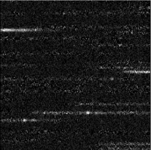
$\stackrel{{\scriptstyle\psfig{width=180.67499pt,angle=-90}\\ \\ \\ }}{{\psfig{width=180.67499pt,angle=-90}}}$

Figure 10: $\rm H\alpha$ spectroscopy of the $z=0.32$ cluster AC114. Top: layout of the spectra in the 9 arcmin FOV, Bottom left: Zoom showing sky-subracted, dispersed image with a couple of $\rm H\alpha$ lines visible. Bottom right: Two sample extracted spectra showing $\rm H\alpha$ and [NII].

Another mode which has been developed for LDSS++ takes the multiplex to an extreme limit by taking advantage of the superb sky-subtraction without a slit. The key idea is to place microslit apertures on large numbers of targets (up to several thousand) without regard to spectral overlap, and possibly even without a blocking filter.

Of course the dispersed sky from such a configuration will generate a very complex, overlapping pattern. However this can still be removed by the nod-shuffle technique, and the residual noise level can be easily calculated. Any features left can have a measurable significance assigned to them.

Why would such observing be useful? Well one example project is illustrated in Figure 11. Here $\sim 2000$ slits were placed on galaxies selected to $R\sim 26$ in a 7 arcmin field called the ‘Herschel Deep Field’ (McCracken  et al. 2000). The sky is removed by nod-shuffle and a noise map is calculated. If a galaxy has strong emission lines then they peak up above the noise map.

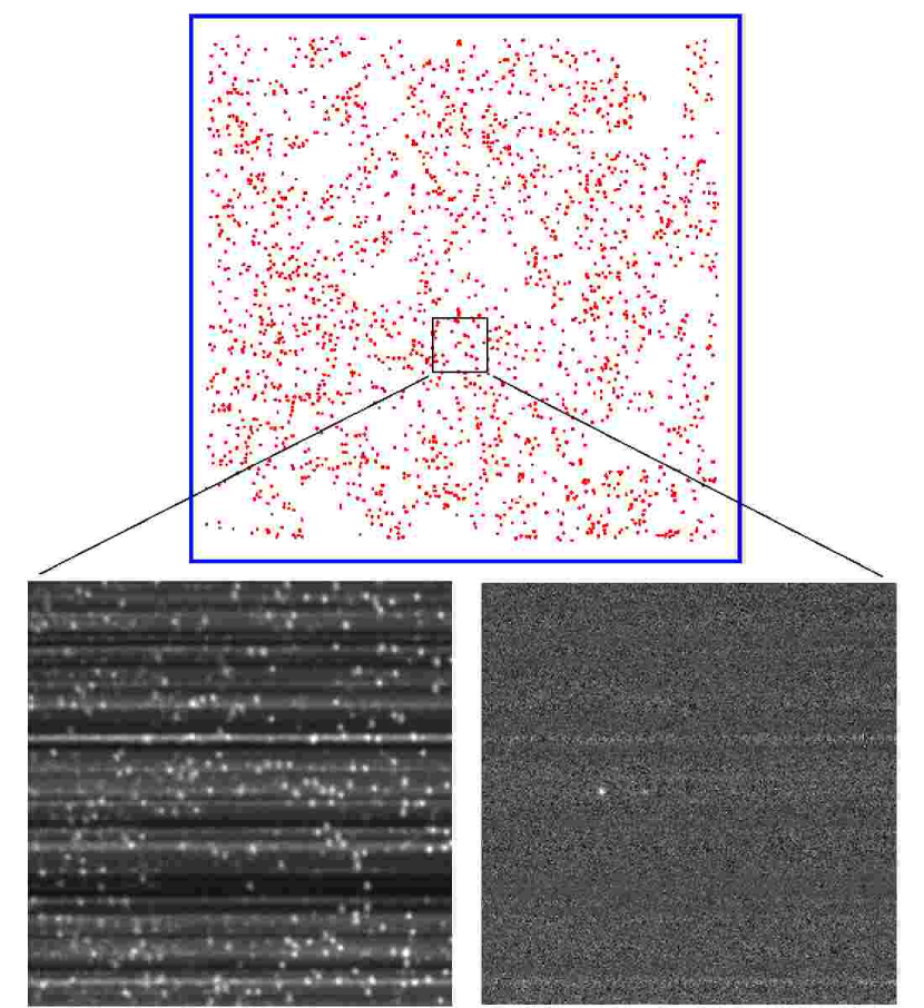
Figure 11: Illustration of a region of data in the ‘Pseudo-slitless’ mode. The full mask (about 7 arcmin) is shown at the top. Slits have been placed on every object with $R<26$ (except near bright foreground stars). The slit density is about 50 arcmin². The lower panels show a region about 1.6 arcmin across zoomed in. Left: before sky-subtraction showing the complex overlapping pattern. Right: after sky-subtraction showing a noise pattern plus some bright emission lines from a low-redshift galaxy. Continuum from some bright objects can also be seen.

Essentially we are searching virtually all galaxies in the field for emission — so it is similar to a slitless grism survey. However we still have a mask in the beam so the level of the sky background is enormously reduced (a factor of 50 in this case) with corresponding increase in signal:noise. Because of the similarity we call this method ‘pseudo-slitless’. Another way of looking at this is we are using our prior knowledge of where galaxies are in the broad-band image to exclude unwanted sky photons. The background is higher than conventional spectroscopy, but more objects are observed simultaneously. In principle these effects cancel exactly, if there are $N$ times more microslits then the average background is $N$ times higher and the exposure has to be $N$ times longer for the same signal:noise. In practice there are gains in efficiency due to factors such as overlap and clustering which complicate slit assigment in the normal case. For the real example in Figure  11 the factor $N\sim 10$.

How does this approach compare against, for example, narrow-band imaging and scanning in wavelength? In the pseudo-slitless mode we are pre-selecting from the broad-band so it is possible to miss pure-emission line objects. If we ignore this difficult to quantify handicap then there is a net gain. Let us assume the tunable-filter instrument has the same absolute throughput as the spectrograph. The pseudo-slitless approach gives a very large wavelength coverage — in our example 5300Å. At a resolution of 20Å then that is needs 265 tunable filter settings. In our example the pseudo-slitless approach has 10 times higher background — so the gain is a factor of $\sim 26$, for the objects searched.

Some data was collected in this mode in August 1999. The project is attempting to quantify the space density of $\rm H\alpha$, $\rm H\beta$, [OII], Ly$\alpha$ line sources at $z=0.2$, 0.6, 1.1, 5.6 respectively (Glazebrook  et al. 2000b).

There is of course an inherent ambiguity: if an emission line is detected how can we determine which microslit it came from? There will be many candidates along it’s dispersion track. This is resolved in two ways: firstly a minimum separation is enforced between slits (e.g. a few arcsec) to allow for errors in the traceback. Secondly the observations are made for different mask orientations on the sky. As the grism is kept fixed we get a different set of tracks. For the observations here positions of 0^∘ and 180^∘ were used: the emission line is dispersed in opposite directions in each case and the correct microslit lies halfway between them.

Finally we note that it is possible to arbitrarily combine the approaches described here. For example in the pseudo-slitless mode blocking filters can also be used: this will limit the spectral coverage but also reduce the background. There is a choice as to whether to go for low or high microslit densities — the latter will mean having to deal with confusion and a higher background.

7 Future prospects

7.1 Nodding with infrared arrays

7.1.1 Prospects for mimicking shuffling directly

Can the nod-shuffle concept be extended to include IR-sensitive devices? We have been asked this question many times — since the OH night sky lines account for 98% of the sky background in the J and H bands this would give major gains. However, infrared arrays are fundamentally different devices from CCDs. In conventional arrays, the pixels are not charge-coupled so that charge cannot be shifted between pixels (Rieke 1994, McLean 1997).

CCDs are monolayer devices where the charge is normally shifted row by row into the read-out (shift) register. Pixels within the read-out register are read out serially towards the output amplifier by means of 2, 3 or 4-phase shift electrodes. In contrast, the Rockwell hybrid arrays are 2-layer devices which use a thin HgCdTe film to collect the light, which in turn is connected pixel-by-pixel via indium bump bonds to a MOSFET multiplexor. Each pixel is addressed in an $(x,y)$ fashion through the use of a row and a column shift register at two edges of the multiplexor. In the ‘source-follower’ multiplexor design, the bump bond makes contact with a MOSFET. When IR photons hit the light-sensitive layer, the electrons are transferred through the bond to the capacitance-storing MOSFET gate. This gate is bordered by a ‘source’ (grounded) and ‘drain’. This circuitry allows for a ‘non-destructive read’ (NDR) of the voltage across the gate. Another FET is attached to the gate to allow every element of the array to be ‘reset’ in a single action.

We have considered possible modifications to the IR array design which would allow for the equivalent of CCD-style charge shuffle operations, i.e. that contains two or more switchable pockets per pixel in which to store charge. Unlike Rockwell arrays, there exist multiplexors which use arrays of FETs as op-amps which simply transfer photogenerated charge to an integrating capacitor (e.g. Kozlowski 1996). One could conceive switching between a pair, or more, of integrating capacitors in which to build up charge sequentially over time.

However, the more connections you attach to the detecting node, the more the capacitance goes up, and therefore the read noise.The array multiplexor already has a higher circuit density compared to CCDs and this would increase it further. This would be a very difficult technology to develop.

7.1.2 Can one use Non-Destructive Reads to facilitate beamswitching?

Figure 12: Illustration of the ‘IR nod-NDR concept’. As counts are accumulated in the NDR mode the telescope is switched between OBJECT and SKY periodically. A double-slope least-squares fit is performed to derive the OBJECT and SKY count rates. It turns out that this is not useful (see text).

We have also considered the question of whether the non-destructive read mode with ramp sampling could be used to mimic shuffling, for example by switching between OBJECT and SKY while sampling up the slope and solving for OBJECT and SKY count rates simultaneously while still allowing readnoise reduction (the main point of ramp sampling). This is illustrated in Figure 12.

We have solved analytically the case for double-slope least square fitting. If $n$ is the total number of reads with error $\sigma$ we find for large $n$ that the error on the OBJECT slope $\sigma_{o}$ is given by:

$$\sigma^{2}_{o}={48k^{2}\sigma^{2}\over n^{3}\Delta t^{2}}$$

where $k$ is the number of OBJECT-SKY sub-intervals (e.g. $k=6$ in Figure 12). If we compare this with the classic single least square formula ($\sigma_{o}=\sqrt{12}\sigma^{2}/n^{3}\Delta t^{2}$), we derive the ratio:

$${\sigma_{o}(\hbox{double)}\over\sigma_{o}(\hbox{single)}}=2k$$

The factor of 2 is the usual beamswitching factor encountered in Section 4. We see the effect of beamswitching is to increase the noise in proportion to the number of switches, this is because the switching reduces the baseline for slope fitting. It turns out for reasonable values of $n$ and $k$ this is not a useful technique. For example suppose the array can be read out every second during a 1800 sec exposure. Single least-squares would give a noise reduction of $\sim 12\times$, if we then beamswitch every 30s this becomes a noise increase of $\sim 4.9\times$.

Finally we note from Section 5.4 that in any case the assumption that the source is of constant brightness and that counts $\propto$ time is very dubious for the sky. The airglow is a stochastic phenomenon with a lot of variation and will deviate from a linear growth. This will generate artificial noise in a line-fitting approach, even with the classical single-line fit. NDR slope-fitting has become a standard technique at many observatories, but the effects of sky-background variations on noise have not been studied.

7.1.3 Physical array shifting

The most reasonable option for mimicking something like charge shuffling is to form two adjacent images at the detector either by nodding the collimator or by a physical movement of the array. The present IR arrays are 1024$\times$1024 pixels in size, although Rockwell are expected to produce 2048$\times$2048 formats in the near future. ‘Detector nodding’ is much the preferred option for a number of reasons. First, a nodding collimator leads to different light paths for the object and sky positions. Secondly, in infrared instrumentation, the collimator must image the pupil onto the cold stop with care. Thirdly, the physical tolerances at the collimator are made much tighter by any focal reduction compared to the tolerances of detector movement. Finally, the array has much the lowest mass of any component of the system, and a 1 Hz movement through a few millimeters is not an excessive strain on the electrical bonds.

An advantage of IR ‘shuffling’ over optical shuffling is that the stored charge is not subject to trapping sites. Furthermore, the detector needs only to be partitioned into two panels rather than the three panels of optical CCDs. A distinct disadvantage is that in IR shuffling the flatfield structure will be different in OBJECT and SKY regions. However this effect can be averaged out by swapping the OBJECT and SKY positions on the array between successive exposures.

For a detector with 18$\mu$m pixels, the physical movement of the array should be accurate to better than 2% of a resolution element (assumed to be 3 pixels). Precision movement to this level is routinely achieved in, say, a mechanism for optical focussing. But within a cryogenic environment, 1$\mu$m accuracy presents a moderate challenge. This seems feasible with either a linear variable differential transformer (LVDT) or a linear encoder. Piezo-electric control at cryogenic temperatures is a more difficult prospect. We note that a well sampled resolution element (say 5 pixels width) may in fact allow wavelength calibration to sufficiently high accuracy between the object and sky exposures that the precision can be relaxed by post-analysis. However, data analysis is greatly simplified by the ability to remove sky accurately by straight subtraction since no interpolation is required.

7.2 Applications to non-contiguous spectroscopy

The nod-shuffle technique allows accurate sky-subtraction without requiring sky spectra which are spatially contiguous on the detector and the sky. Thus it is particularly suitable for non-contiguous optical systems such as fiber spectrographs and integral field unit spectrographs (IFUs), both fiber based and non-fiber based.

Application of fibers to faint spectroscopy have been limited by sky-subtraction accuracies of typically 3% (Wyse & Gilmore 1992), which are due to variable fiber transmission. The nod-shuffle technique can be applied to fiber spectrographs providing there is spare room on the detector as outlined earlier, the 2D shuffled subframe of SKY spectra through the fibers is simply subtracted from the 2D OBJECT subframe.

Due to the quasi-simultaneity the effect of varying fiber throughput, which varies on a much long timescale (hours), will cancel out as the sky is observed through exactly the same fibers. At the AAT we have already experimented with nod-shuffle using the Two Degree Field fiber spectrograph and have obtained shot noise limited subtraction implying systematics $<<1\%$ (Glazebrook  et al. 1999).

The application to IFU’s is also straight-forward. Accurate sky-removal is achieved by subtracting the shuffled frames before individual IFU element spectra are extracted and assembled to make a data cube. Just like the slit case the object could be nodded between two positions on the IFU, or the nod throw could be large enough to move the whole IFU to clear sky. While the effect of calibration of elements on sky-subtraction is eliminated, it must still be solved if accurate spectro-photometry is desired.

7.3 Ultra-Deep spectroscopic exposures

The promise of nod-shuffling is of course that the extreme precision of sky cancellation will allow very very long deep spectroscopic exposures. It is interesting to compare ground-based spectroscopy with space astronomy (X-ray, IR, etc.). In the latter it is common to see total exposures of many days to weeks in total, whereas in the former it is rare to see total exposures of longer than a night’s observing.

Why is this? The answer is because of the high sky background then one reaches a limit in only a few hours observing where one is dominated by the systematics of how well one can remove it. This is doubly important because the sky spectrum exhibits extraordinarily complex structure. Also as we have seen in Section 5.1 there are a large number of seperate instrumental effects which all operate at the $0.5-1\%$ level.

The beauty of the nod-shuffle technique is that it is a perfectly differential experiment and all of these effects are removed simultaneously from the sky-subtraction process. They still affect the object spectrum, but that is far less important compared to the random noise.

The question arises then will the nod-shuffle technique permit the use of ultra-deep exposures, lasting $10^{5}-10^{6}$ secs, for optical spectroscopy? We believe it can. At the level of sky-subtraction precision demonstrated we estimate that one could obtain a good spectrum of a $I_{AB}=27.2$ galaxy (i.e. $3\sigma$ above the sky limit). At a resolution of $R\sim 800$ one could reach this in a 200,000 sec exposure (7 nights) on a 10m telescope with a 35% efficient spectrograph. Using microslits one could squeeze many parallel targets into even a small field.

We re-emphasize that we believe our current sky-subtraction accuracy is only an upper limit to what can be achieved. The sky-background can be reduced further by observing at higher-resolution so the OH lines do not dominate the spectrum. The intra-OH continuum variations may be far less rapid so even greater accuracy could be obtained. Assuming we could reach $10^{-4}$ of the sky at a resolution $R=5000$, then faintest object would be $I_{AB}=29$. This could be reached in a $10^{8}$ second exposure (3 years!) or a more reasonable $10^{7}$ exposure if the spectrum was post-hoc rebinned to $R=500$.

30–50m telescopes are being planned at the time of writing, these would reach the same limits an order of magnitude faster. We emphasize that without nod-shuffle, or equivalent, techniques these telescopes would reach the systematic limit for spectroscopy in a mere one hour exposure!

8 Summary and Conclusions

We have explained the virtues of the nod-shuffle technique for CCD-based optical spectroscopy: we reach a new level of sky-subtraction precision of 0.04%. This is in accord which predictions from a reasonable physical model of atmospheric airglow.

This technique also permits a great increase in the multiplex gain of multi-slit spectrographs we have quantified those gains and showed that they are the most in high-object density regimes.

We have outlined our thoughts on IR techniques equivalent to nod-shuffle. Possibly new circuit designs would allow charge storage but would need to be developed. Given the importance of IR spectroscopy on future large telescopes the scientific case for doing so is strong. Failing this we have outlined a less satisfactory, but still useful concept, for physically moving the IR array.

For very large telescopes (10m and greater) the precision of sky-subtraction is a real barrier for ultra-deep spectroscopic exposures. The systematic limit of ordinary slit subtraction is reached in only a few hours. The nod-shuffle technique offers a remedy, and promises the possibility of extremely long exposures, it’s ultimate performance remains to be explored.

References

- (1)
- (2) Abrams, M.C., Davis, S.P., Rao, M.L.P., Engleman, R., Brault, J.W. 1994, ApJS, 93, 351
- (3)
- (4) Adams, J.D. & Skrutskie, M.F. 1997, preprint
- (5)
- (6) Barden, S.C., Arns, J.A. & Colburn, W.S. 1998, In Optical Astron. Instrumentation, Proc. SPIE, 3355, 866
- (7)
- (8) Barnes, J.A. & Allan, D.W. 1966, Proc. I.E.E.E. 54, 176
- (9)
- (10) Bland-Hawthorn, J., 1994, Anglo-Australian Tunable Filter, internal document (see http://www. aao.gov.au/local/www/jbh/ttf/docs/aatf.ps.gz)
- (11)
- (12) Bland-Hawthorn, J., 1995, In Tridimensional Spectrscopic Methods in Astrophysics, ed. G. Comte& M. Marcelin, ASP Conf., 71, 369
- (13)
- (14) Bland-Hawthorn, J. & Barton, J. 1995, AAO Newsletter 74, 10
- (15)
- (16) Bland-Hawthorn J., Veilleux S., Cecil G. N., Putman M. E., Gibson B. K., Maloney P. R., 1998, MNRAS, 299, 611
- (17)
- (18) Bland-Hawthorn, J., Glazebrook, K., Barton, J.R., Waller, L.G. & Farrell, T.J. 2000, in preparation
- (19)
- (20) Blouke, M.M., Yang, F.H., Heidtmann, D.L. & Janesick, J.L. 1988, In Instr. for Ground Lased Optical Astron., Present and Future, Proc. SPIE.
- (21)
- (22) Comte, G., Marcelin, M., 1995, Tridimensional optical spectroscopic methods in astrophysics, Proceedings of the IAU Colloquium 149, ASP Conference series Vol. 71.
- (23)
- (24) Couch, W.J., Balogh, M.L., Bower, R.G., Smail, I.S., Glazebrook, K., Taylor, M., 2000, ApJ, in press
- (25)
- (26) Cuillandre J. C., Fort B., Picat J. P., Soucail J. P., Altieri B., Beigbeder F., Duplin J. P., Pourthie T., Ratier G., 1994, A&A, 281, 603
- (27)
- (28) Dressler, A. 1984, ApJ, 286, 97
- (29)
- (30) Fossum, E.R. 1997, IEEE Trans. Elec. Dev., 44, 1689
- (31)
- (32) Gardner J.P., Satyapal S., ApJ, in press
- (33)
- (34) Glazebrook, K., Ellis, R. S., Colless, M. M, Broadhurst, T. J., Allington-Smith, J. R., Tanvir, N. R., 1995, MNRAS, 273, 157
- (35)
- (36) Glazebrook K. 1998, AAO Newsletter 87, 11
- (37)
- (38) Glazebrook K., Bland-Hawthorn J., Farrell T. J., Waller L., Barton J. R., Lewis I. J., 1999, AAO Newsletter, 90, 11
- (39)
- (40) Glazebrook, K. 2000, In Encyclopaedia of Astronomy and Astrophysics, (MacMillan and Inst. of Physics Publ.,) ed. P.G. Murdin
- (41)
- (42) Glazebrook, K. et al. 2000a, in preparation
- (43)
- (44) Glazebrook, K. et al. 2000b, in preparation
- (45)
- (46) Hogg D. W., Pahre M. A., Mccarthy J. K., Cohen J. G., Blandford R., Smail I., Soifer B. T., 1997, MNRAS, 288, 404
- (47)
- (48) Janesick, J. & Elliott, T. 1992, In Astronomical CCD Observing and Reduction Techniques, ed. S.B. Howell, ASP Conf., 23, 1
- (49)
- (50) Kondratyev, K. Ya. 1969, Radiation in the Atmosphere, (New York: Acad. Press)
- (51)
- (52) Kozlowski L.J., 1996, SPIE, 2745, 2
- (53)
- (54) Leinert, Ch., Bowyer, S., Haikala, L. K., Hanner, M. S., Hauser, M. G., Levasseur-Regourd, A.-Ch., Mann, I., Mattila, K., Reach, W. T., Schlosser, W., Staude, H. J., Toller, G. N., Weiland, J. L., Weinberg, J. L., Witt, A. N., 1998, A&AS, 127, 1
- (55)
- (56) Lemonier, M. & Piaget, C. 1983, IEEE Trans. Elec. Dev., 30, 1414
- (57)
- (58) McCracken H. J., Metcalfe N., Shanks T., Campos A., Gardner J. P., Fong R., 2000, MNRAS, 311, 707
- (59)
- (60) McLean, I.S., Cormack, W.A., Herd, J.T. & Aspin, C. 1981, In Solid State Imagers for Astronomy, ed. J.C. Geary and D.W. Latham, Proc. SPIE, 290, 155
- (61)
- (62) McLean, I.S. 1997, Electronic Imaging in Astronomy: Detectors and Instrumentation (Wiley-Praxis Series in Astronomy and Astrophysics)
- (63)
- (64) Rieke, G.H. 1994, Detection of Light: from the Ultraviolet to the Submillimetre, (Cambridge University Press).
- (65)
- (66) Ramsay, S.K., Mountain, C.M. & Geballe, T.R. 1992, MNRAS, 259, 751
- (67)
- (68) Sembach K.R., Tonry J.L., 1996, AJ, 112, 797
- (69)
- (70) Smail, I., Hogg, D.W., Lin, Y., & Cohen, J.G. 1995, ApJ, 449, L105
- (71)
- (72) Stockman, H.S. 1982, In Instrumentation in Astronomy IV, ed. D.L. Crawford, Proc. SPIE 331, 76
- (73)
- (74) Szeto, K., Stilburn J., Bond T., Roberts S., Sebesta J., Saddlemyer L., 1996, In Optical Telescopes of Today and Tomorrow, SPIE, 2871, 1262
- (75)
- (76) Wynne, C.G. & Worswick, S.P., 1988, The Observatory, 108, 161
- (77)
- (78) Wyse R. F. G., Gilmore G., 1992, MNRAS, 257, 1
- (79)