Stellar Population Analysis from Broad-Band Colours

We have developed an analytical method to investigate the stellar populations in a galaxy using the broad-band colours. The method enables us to determine the relative contribution, spatial distribution and age for different stellar populations and gives a hint about the dust distribution in a galaxy.
We apply this method to the irregular galaxy NGC 3077, using CCD images in U, B , V and R filters. END Galaxies: Stellar populations – Galaxies: individual (NGC 3077) END

1 Introduction

The investigation of stellar populations in a galaxy using broad-band colours is based on an analysis of the distribution of stars in the colour magnitude diagram (CMD), and the comparison of the observed CMD with a set of model CMDs. In more distant galaxies, individual stars are difficult to observe, and hence one must interpret the integrated light in terms of the stellar populations and use colours of model populations for comparison. Papers using the last-mentioned approach are becoming more frequent recently. For instance, Kong et al. (2000) used a set of 13 intermediate-band colours to get information on the distribution of age, extinction and metallicity in M81, assuming a population of stars of equal age in each pixel. Bell et al (1999) and Abraham et al (1999) analysed the pixel-by-pixel colour distribution to get the overall star formation history, comparing the colours with theoretical predictions for populations with various time-scales $\tau$ of the star forming process.

In contrast, Notni and Bronkalla (1984) derived the population distribution in the inner regions of M82 assumimg two distinct populations (each with small $\tau$) in each pixel in their analysis of photographic data. Similarly, the integrated colour for a sample of dwarf galaxies was interpreted by Almoznino and Brosch (1998) as a combination of a young (3-13Myr) and an old (1-2 Gyr) stellar populations. They get their conclusion by calculating some combinations for the integrated light of two populations with different ratio. We start, the other way round, from the observed light in every point in the galaxy and try to decompose this light into its contributions from the two stellar populations by solving the equations which describe the combined colours. The method enables us to estimate the age and the extinction of the population I and the contribution of both populations I and II to the observed light.

In the present paper, the mathematical presentation of the method is given in section 2. A short error analysis in the determination of age and relative contribution of different populations is discussed in section 3. In section 4, an application of the method using CCD observations of the irregular galaxy NGC 3077 is presented. The conclusion will be given in section 5. The observations used in this work and their reduction are presented in our preceeding paper in this issue (Abdel-Hamid & Notni 2000, HN1 hereafter).

2 Derivation of the relative abundance of two populations

Let us assume that the observed light of a galaxy comes from only two stellar populations with different colours, i.e. with different age, metallicity, etc. A graphical presentation of the line along which the colour changes if two given populations mix in various proportions is given in Figure 1. P2 refers to the colour of an old population and P1 to the colour of the young population. Both P1 and P2 mix along the line which connects them to give the observed colour.

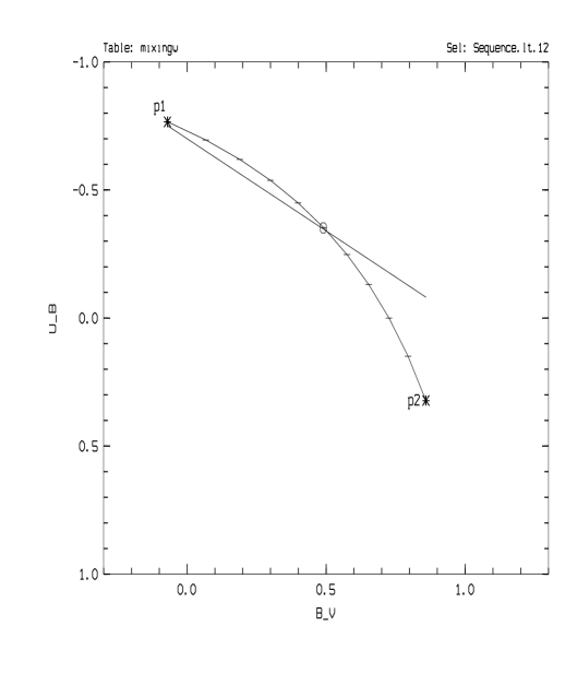
Figure 1: A mixing track in the UBV colour-diagram. Population I (p1) and population II (p2) mix and produce the observed colour along the curved track. Ticks on the mixing track represent different contributions of the populations in the observed light ($\beta$), step = 0.1. The open circle marks an observed colour, in which 50% of its total light comes from the population I (p1). The solid line is a reddening vector.

In order to derive the required relations which describe the mixing-tracks of the two stellar populations, we start with some definitions. The suffixes m, I and II refer to total (measured), population I and population II intensity, respectively. The colour indices are defined with respect to that of population II.

$\triangle(U-B)_{m}$	=	$(U-B)_{m}-(U-B)_{II}$,	$\triangle(U-B)_{I}$	=	$(U-B)_{I}-(U-B)_{II}$
$\triangle(B-V)_{m}$	=	$(B-V)_{m}-(B-V)_{II}$,	$\triangle(B-V)_{I}$	=	$(B-V)_{I}-(B-V)_{II}$
$\triangle(B-R)_{m}$	=	$(B-R)_{m}-(B-R)_{II}$,	$\triangle(B-R)_{I}$	=	$(B-V)_{I}-(B-V)_{II}$
$\triangle(B-\hskip 2.84526ptI)_{m}$	=	$(B-\hskip 2.84526ptI)_{m}-(B-\hskip 2.84526ptI)_{II}$,	$\triangle(B-\hskip 2.84526ptI)_{I}$	=	$(B-\hskip 2.84526ptI)_{I}-(B-\hskip 2.84526ptI)_{II}$

Then we define the following intensity relations:

$$\frac{u_{m}}{b_{m}}=\frac{u_{I}\cdot e^{-\tau_{u}}+u_{II}}{b_{I}\cdot e^{-\tau_{b}}+b_{II}}\quad\mbox{,}\quad\frac{b_{m}}{v_{m}}=\frac{b_{I}\cdot e^{-\tau_{b}}+b_{II}}{v_{I}\cdot e^{-\tau_{v}}+v_{II}}$$

$$\frac{b_{m}}{r_{m}}=\frac{b_{I}\cdot e^{-\tau_{b}}+b_{II}}{r_{I}\cdot e^{-\tau_{r}}+r_{II}}\quad\mbox{,}\quad\frac{b_{m}}{i_{m}}=\frac{b_{I}\cdot e^{-\tau_{b}}+b_{II}}{i_{I}\cdot e^{-\tau_{i}}+i_{II}}$$

where u,b,v,r and i are the dereddened intensities in the corresponding band and for the corresponding population, while that with suffix $m$ are the observed total light intensities. $\tau_{b}$ is the optical thickness in the B band.
Note that only population I is assumed to suffer extinction, equivalent to the assumption of a typical galaxy structure governed by a flat young population associated with dust structures, embedded in an old population mainly outside the extinction layer.
Converting the above equations to magnitudes we get

$$(U-B)_{m}=(U-B)_{II}-2.5\log\left(\frac{\alpha X_{0}e^{-\tau_{u}}+1}{\alpha e^{-\tau_{b}}+1}\right)$$

$$(B-V)_{m}=(B-V)_{II}-2.5\log\left(\frac{\alpha e^{-\tau_{b}}+1}{\alpha X_{1}e^{-\tau_{v}}+1}\right)$$

$$(B-R)_{m}=(B-R)_{II}-2.5\log\left(\frac{\alpha e^{-\tau_{b}}+1}{\alpha X_{2}e^{-\tau_{r}}+1}\right)$$

$$(B-I)_{m}=(B-I)_{II}-2.5\log\left(\frac{\alpha e^{-\tau_{b}}+1}{\alpha X_{3}e^{-\tau_{i}}+1}\right)$$

with

$$\alpha=\frac{\beta_{b}}{e^{-\tau_{b}}-\beta_{b}\cdot e^{-\tau_{b}}}\quad\mbox{ and}\quad\beta_{b}=\frac{b_{I}\cdot e^{-\tau_{b}}}{b_{m}}=\frac{b_{I}\cdot e^{-\tau_{b}}}{b_{I}\cdot e^{-\tau_{b}}+b_{II}}$$

$$\frac{u_{I}}{b_{I}}=X_{0}\cdot\frac{u_{II}}{b_{II}}\quad\mbox{,}\quad\frac{b_{II}}{v_{II}}=X_{1}\cdot\frac{b_{I}}{v_{I}}\quad\mbox{,}\quad\frac{b_{II}}{r_{II}}=X_{2}\cdot\frac{b_{I}}{r_{I}}\quad\mbox{and}\quad\frac{b_{II}}{i_{II}}=X_{3}\cdot\frac{b_{I}}{i_{I}}$$

and

$$X_{0}=dex(-0.4\triangle(U-B)_{I})\quad\mbox{,}\quad X_{1}=dex(0.4\triangle(B-V)_{I})$$

$$X_{2}=dex(0.4\triangle(B-R)_{I})\quad\mbox{,}\qquad X_{3}=dex(0.4\triangle(B-I)_{I})$$

Here $e^{-\tau_{\lambda}}=dex(-0.4\cdot A_{\lambda})$, and using a total to selective extinction ratio of $R_{v}=3.1$, the colour excess relations for other wavelength bands is $E_{u-b}=0.72E_{b-v}$, $E_{v-i}=1.25E_{b-v}$ and $E_{v-r}=0.62E_{b-v}$ (Grebel & Roberts 1995).
Note that the X’s are functions of the colours of both populations I and II.
We get:

$$(U-B)_{m} = (U-B)_{II}-2.5\log\left(1-\beta_{b}+\beta_{b}\cdot 10^{(-0.288E_{b-v})}\cdot 10^{(-0.4\triangle(U-B)_{I})}\right)$$

$$(B-V)_{m} = (B-V)_{II}+2.5\log\left(1-\beta_{b}+\beta_{b}\cdot 10^{(0.4E_{b-v})}\cdot 10^{(0.4\triangle(B-V)_{I})}\right)$$

$$(B-R)_{m} = (B-R)_{II}+2.5\log\left(1-\beta_{b}+\beta_{b}\cdot 10^{(0.648E_{b-v})}\cdot 10^{(0.4\triangle(B-R)_{I})}\right)$$

$$(B-I)_{m} = (B-I)_{II}+2.5\log\left(1-\beta_{b}+\beta_{b}\cdot 10^{(0.9E_{b-v})}\cdot 10^{(0.4\triangle(B-I)_{I})}\right)$$

A common wavelength band (e.g. B in our case) in the colour indices is essential to get the relative abundance of the populations in the observed intensity.
In general form the observed colour index is given as:

$$(B-\lambda)_{m}=(B-\lambda)_{II}+2.5\log\left(1-\beta_{b}+\beta_{b}\cdot 10^{c\cdot E_{b-v)}}\cdot 10^{(0.4\triangle(B-\lambda)_{I})}\right)$$ (1)

where the colour indices are a difference between a certain wavelengthband ($\lambda$) and the B-band. $c$ is a constant, its value depends on the colour excess relations for the wavelength bands.
From the above equations, the required relation for the relative light-contribution of population I, $\beta_{b}$, is:

$$\beta_{b} = \frac{1-A}{1-X_{0}\cdot dex(-0.288E_{b-v})}$$

$$= \frac{1-B}{1-X_{1}\cdot dex(0.4E_{b-v})}$$

$$= \frac{1-C}{1-X_{2}\cdot dex(0.648E_{b-v})}$$

$$= \frac{1-D}{1-X_{3}\cdot dex(0.9E_{b-v})}$$

with

$$A=dex(-0.4\triangle(U-B)_{m})\qquad\mbox{,}\qquad B=dex(0.4\triangle(B-V)_{m})$$

$$C=dex(0.4\triangle(B-R)_{m})\qquad\mbox{,}\qquad D=dex(0.4\triangle(B-I)_{m})$$

A, B, C and D are functions of the observed and population II colours.

If we replace in equations 1 the colour indices of both populations I and II by the age of each of them, then these equations contain only four unknowns (age of population I, age of population II, $\beta$ and $E_{b-v}$). The system becomes mathematically solvable, whenever four observed colour indices are used. To provide the age dependence of the broad-band colours of the stellar populations, a population synthesis model is used. Having only three colour indices, the system of equations cannot be solved without further assumptions, however. In many cases, including NGC3077, the colour of population II, i.e. its age, can be determined independently from some outer regions of the galaxy. This reduces the number of unknowns to 3 and the system becomes solvable already with only three measured colours. In NGC3077, the colour of population II is assumed to be the mean of the data clustering around U-B = 0.3 mag, B-V = 0.85 mag and B-R = 1.4 mag in the colour diagrams, corresponding to an age of 2..4x10⁹ years, see Figure 6 and HN1. An even more restricted solution of the problem was used by Notni and Bronkalla (1984) to analyse the distribution and extinction of two populations of known reddening-free index [Q=(U-B)-0.65(B-V)] in the galaxy M82 from only two colour indices.

3 Short error analysis

For the typical assumption of a known colour (or age) of population II, we check the influence of errors in this assumption on the deduced parameters $age(popI)$ and $\beta$, assuming for this test zero extinction. We use the UBV diagram and the theoretical age line of Bressan et al. 1994 (hereafter BCF94), illustrated in Figure 4. We try to estimate the error in the estimation of the age of the population I, (the left panels in the Figures 2 and 3), and on the ratio $\beta$ (the right panels).

If the assumed age of population II goes from 2 to 10 Gyr, (corresponding to a range in $(B-V)_{II}$ from 0.80 to 1.01 or $(U-B)_{II}$ from 0.24 to 0.59), this will produce an error in the estimation of the age of population I between 0 (uppermost curves in Figures 2 and 3) and 9 Myr (lowest curves), and an error in the ratio $\beta$ between 0 and 14% respectively, where the amount of error depends on the location of the test points in the two-colour diagrams. At lower ages, if the estimated population II age moves between 1 and 2 Gyr, the results are less certain; the error may be as high as a factor of four in the age of population I and 20% for $\beta$.

In the region of practical interest, where the age of population II is 3$\pm 1$ Gyr, the estimation of the age of population I is accurate to about 4 Myr and $\beta$ by about 7% in the average. .

The same Figures can also be used to get the influence of errors in the observed mixed colours on these parameters. The dotted line in Figures 2 and 3 is used for this; it is valid for a combination of an old population with an age of 3 Gyr and a young population (characterized by age or its contribution $\beta$), which will give the observed colours $(B-V)_{m}$ and $(U-B)_{m}$. The movement of the observed colours by 0.1 on the dotted line, i.e. if there is an error of 0.1 in the observed colours, leads to an error of the estimation of $\beta$ by an amount of 10% and of the age of population I by 20 Myr in the average.

Figure 2: The effects of change of the assumption of the colour (or, equivalently, age) of population II for eight test data points with constant (U-B)m = -0.2 and (B-V)m ranging from 0.1 to 0.45, on (a) the estimation of the age of population I, in Myr, and (b) its contribution percent $\beta$, in the observed intensity. The population II is represented, along the abscissa, by its age or, alternativly, its colours, assumed changing along the age-line for z=0.02 of the BCF94 model. The dotted line gives the influence of errors in the observed mixed colours on the deduced parameters $age(popI)$ and $\beta$, see text.

Figure 3: As Figure 2 , but for a set of observed points with constant (B-V)m = 0.3 and (U-B)m ranging from - 0.05 to - 0.40.

4 Applying the method to the observations

We analyse the observational data for NGC 3077 using as an age reference line the models of BCF94, as illustrated in Figure 4.

In the UBV-diagram, the mixing curve of the two populations is inclined to the age line, but about parallel to the reddening line. This leads to an easy estimate of the age of population I, but it is impossible to distinguish reddening from the effect of the varying contributions of the two populations ($\beta$, ticks in the Figures) using only these colour indices (U-B and B-V). For every age estimation there are many possible combinations of $\beta$ and $E_{b-v}$. Therefore, another two-colour diagram is required in order to get discrete values of age, $\beta$ and $E_{b-v}$ for each observed colour. We use the two-colour diagram B-V / B-R for this purpose.

A MIDAS iteration subroutine is used to solve the system of equations 1 as follows: for each age value in some age range of the young population I, its colour indices are read as input parameters; for population II constant colours corresponding to an age of 3x$10^{9}$ yrs (z=0.02) are used. Then we calculate three $\beta$ images, one for each observed colour, and the standard deviation of these values in every pixel, the ($\sigma_{\beta}$) image. This is done for 14 different age values of population I, ranging from 4x$10^{6}$ to $10^{8}$ yrs. From these 14 $\sigma_{\beta}$ images the subroutine looks for the minimum value of $\sigma_{\beta}$ at each pixel and writes its corresponding age, ${\beta}$ and $\sigma_{\beta}$, at this position in three new images, named for example $Age$0, $\beta$0 and $\sigma_{\beta}$0 (for an assumed value of extinction $E_{b-v}$ = 0). In a second step the program repeats these calculations for a range of extinction values, in terms of $E_{b-v}$ from 0 to 1.0, step 0.1. This will give for each parameter set ($age$, ${\beta}$ and $\sigma_{\beta}$) 10 images. From these 10 $\sigma_{\beta}$ images the program searches again the minimum $\sigma_{\beta}$ and writes this value and the corresponding $age$, $\beta$ and $E_{b-v}$ values in the corresponding position in four new images. The three images $\beta$, $age$ and $E_{b-v}$ are the required solution of equation 1 for each pixel. The $\beta$ image gives at every pixel the contribution of population I in the observed light (in B filter in this case), while the $age$ and $E_{b-v}$ images give the distribution of the age of population I and its associated extinction in the field of interest.

We now apply the above method to the central region of NGC 3077 ($\sim$1 kpc) with the aim to get the distribution of the young population I and its age distribution and extinction. We use intrinsic colours for the young population from the population synthesis model data of Bressan et al. 1994, choosing a metallicity value of z=0.05, to put a formal metallicity difference between the two populations. (For the old population II solar metallicity, z=0.02, was assumed throughout this paper following Chromey 1974). The influence of this choice for the metallicity on the results is minor, however, since the difference of the age lines in the region of interest – the young populations – is small, as can be seen from Figures 4 and 6.

First we analyse the overall contribution of both populations I and II to the observed B light using the intensity ratio ($\beta$) and its complementary, (1-$\beta$). These distributions were fitted by isophote ellipses using a Fortran program to extract the characteristic parameters of the two populations. Figure 6 gives the surface brightness distribution of both populations I and II in comparison with that of the whole galaxy. The contribution of population I is highest in the centre, steeply decreasing with distance from the centre. Population II is present also in the central part but becomes the dominant population in the outer part.

Figure 7 shows the age distribution of the population I, as obtained using the mentioned method. The Figure depicts an interrupted ring structure of a very young population, age between 13 and 50 Myr (follow the inner dark grey structure in the figure). A spot of age 4 Myr is embedded in the left part of the ring (the darkest spot in the figures). This spot lies at the position of the prominent young star cluster in NGC 3077 mentioned by Price and Gullixson 1989. It can also immediately be seen on an HST image.

This structure is superposed on a homogeneous background distribution of an older population I aged about 100 Myr (the outer dark grey background). This distribution suggests that several successive recent star formation events occured in the central region of NGC 3077.

The contribution of the population I in the observed light shown by the dashed contours in Figure 7 is highest in the centre and becomes lower going outward to reach 10% at nearly $60^{\prime\prime}$ from the centre (the boundary of the central region of NGC 3077, see also HN1).

The extinction distribution of population I in the central region of NGC 3077 is shown in Figure 8 in terms of $E_{b-v}$. $E_{b-v}$ isophotes from 0.1 to 0.5 step 0.1 mag are superimposed on the age variation image. They are correlated with the ring structure of the age distribution. A high extinction exists at south-west of the young star-cluster (the dark spot). At this location lies the prominent dark cloud in NGC 3077.

Figure 4: The mixing-tracks in two different colour diagrams, with two mixing curves joining an old population (3Gyr) with two age limits of the young population (3, 100 Myr). The points in the left panel are observed colours in the central region. Ticks are $\beta$ values, step 0.1 (see text). Dotted and long dashed curves are population synthesis models with Z = 0.02 and Z = 0.05, respectively (BCF94). The solid thick line is a reddening vector.

Figure 5: Two-colour diagram of the population synthesis models by BCF94 and LT78 in comparison. The symbols refer to the age of the populations, different lines are different metallicities as follows: solid (Z = 0.05), dotted (Z = 0.02), short dashed (Z = 0.008) and long dash-doted (Z = 0.001) for BCF94. The thick solid line is the Larson & Tinsley model 1978 with solar metallicity, Z = 0.02 (for comparison).

Figure 6: B surface brightness ($mag/arcsec^{2}$) for population I (stars) and II (crosses) and for the whole galaxy (ellipses) as a function of the semi-major axis length, in arcsec. The dashed line shows the level of the night sky brightness in B.

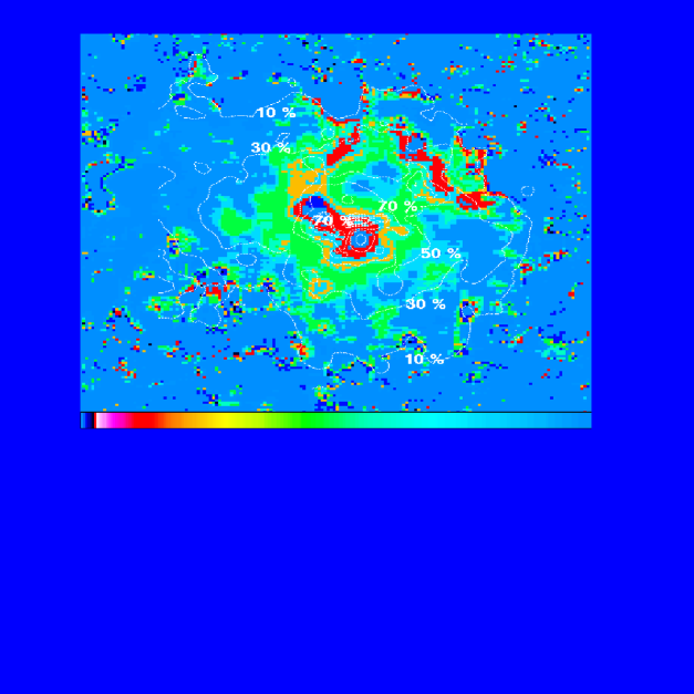
Figure 7: The distribution of the age of population I in the central region of NGC 3077 (crudely quantizised). The darkest spot in the middle left side is a prominent star cluster with age of 4 Myr. Age coding is as follows: dark grey (inner regions) (13 Myr), light grey (inner regions) (25 Myr), middle grey (50 Myr), light grey (outer regions) (80 Myr) and dark grey outer background (100 Myr). Contours superposed on the age distribution show the contribution of population I to the observed B light. North is up and east is to the left. The image size is 1.5x1.5 kpc.

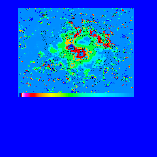
Figure 8: The $E_{b-v}$ contours from 0.1 to 0.5, step 0.1 superposed on the age distribution of population I in the central region. North is up and east is to the left. The image size is 1.5x1.5 kpc.

5 Conclusion

We present a simple method for deducing the relative contributions of the stellar populations of galaxies by an analysis of their colours. We solve the ’mixing equations’ (by iteration) for the case of two populations of markedly different age in NGC 3077.

For NGC 3077, the main results of this paper can be summarized as follows:
- We derive the spatial distribution of both populations together with an estimate of their age and an extinction estimate for population I.
- The young population is concentrated in the central region of NGC 3077. Its contribution to the observed light decreases going out from the centre.
- The youngest structures, aged 10-20 Myr, concentrate along a ringlike structure, associated with dust. The ring breaks up into discrete star-forming clumps.
- An age gradient for the young population in the central region of NGC 3077 is found, ages range from 4 Myr in the centre to 100 Myr at a projected radial distance of 1 kpc. Such age variation reflects the occurence of different events of star formation, probably starting from the beginning of the encounter with M81 (a few hundred million years) until now.
- The prominentest star cluster in the central region is found to have the lowest age, about 4 Myr.

The abovementioned results encourage us to use our method to study the stellar populations in faint galaxies using only the familiar broad band colours.