Peering through the dust: Evidence for a supermassive Black Hole at the nucleus of Centaurus A from VLT IR spectroscopy

Abstract

We used the near infrared spectrometer ISAAC at the ESO Very Large Telescope to map the velocity field of Centaurus A (NGC 5128) at several position angles and locations in the central 20″ of the galaxy. The high spatial resolution ($\sim 0\farcs 5$) velocity fields from both ionized and molecular gas ($\mathrm{Pa}\beta$, $[\mathrm{Fe}\,\textsc{ii}]$, $\mathrm{Br}\gamma$ and $\mathrm{H}_{2}$) are not compromised by either excitation effects or obscuration. We identify three distinct kinematical systems: (i) a rotating ”nuclear disk” of ionized gas, confined to the inner 2″, the counterpart of the $\mathrm{Pa}\alpha$ feature previously revealed by HST/NICMOS imaging; (ii) a ring-like system with a $\sim 6\arcsec$ inner radius detected only in $\mathrm{H}_{2}$  likely the counterpart of the 100$\,\mathrm{pc}$-scale structure detected in CO by other authors; (iii) a normal extended component of gas rotating in the galactic potential. The nuclear disk is in keplerian rotation around a central mass concentration, dark ($M/L>20\,\mathrm{M}_{\odot}/\mathrm{L}_{\mathrm{K}\odot}$) and point-like at the spatial resolution of the data ($R<0\farcs 25\sim 4\,\mathrm{pc}$). We interpret this mass concentration as a supermassive black hole. Its dynamical mass based on the line velocities and disk inclination ($i>15\arcdeg$) is $M_{\bullet}=2^{+3.0}_{-1.4}\times 10^{8}\mathrm{M}_{\odot}$. The ring-like system is probably characterized by non-circular motions; a ”figure-of-8” pattern observed in the $\mathrm{H}_{2}$ position-velocity diagram might provide kinematical evidence for the presence of a nuclear bar.

1 Introduction

Mass accretion onto a supermassive black hole (BH) is widely accepted as the most likely mechanism for powering Active Galactic Nuclei (AGN). It provides a simple and efficient way to produce the necessary large amount of energy in a small volume. Demonstrating the existence of supermassive black holes and measuring their masses has thus been a crucial element in confirming the standard view of AGNs.

Over the last few years, there have been direct dynamical mass determinations for BHs in nearby galaxies in sufficient numbers and with sufficient accuracy to enable detailed demographic studies (e.g. the recent reviews by Macchetto, 1999; Ho, 1998; Ford et al., 1997; van der Marel, 1997; Kormendy & Richstone, 1995). The possible correlation observed between the mass of the BH and that of the host spheroid (either the bulge of a spiral galaxy, or the entire mass of an elliptical galaxy) has prompted serious studies of the relationship between BH growth and host galaxy evolution (Magorrian et al., 1998; Richstone et al., 1998).

The nuclei of many AGNs and normal galaxies alike are heavily obscured by dust, making it difficult to study kinematics at visible wavelengths. For example, the 3CR HST snapshot survey has shown that the nuclei of radio galaxies are often covered by foreground dust lanes (De Koff et al., 1996; Martel et al., 1999). This has been further confirmed by other sensitive surveys with WFPC2 and NICMOS (Malkan, Gorjian & Tam, 1998; Regan & Mulchaey, 1999). Such dust obscuration can distort both absorption line and emission line velocity field measurements to such an extent that reliable BH mass estimates are difficult or impossible using optical data alone. IR spectroscopy is thus increasingly important to continue to find and measure the masses of black holes in active galaxies.

Centaurus A (NGC5128), the closest active giant elliptical galaxy, nicely illustrates the problem of dust obscuration. At optical wavelengths, its nucleus is made almost completely invisible by its dust lane, rich in molecular and ionized gas, which obscures the inner half kiloparsec of the galaxy. A comprehensive recent review on the properties of the galaxy and of its AGN is presented by Israel (1998).

The kinematics of the ionized gas was mapped in $\mathrm{H}\alpha$ by Bland, Taylor & Atherton (1987) and subsequently modeled by Nicholson, Bland-Hawthorn & Taylor (1992, hereafter NBT92) who showed that the dust lane can be kinematically and morphologically explained with a thin warped disk geometry. On the assumption of closed circular orbits, the $\mathrm{H}\alpha$ velocity field is consistent with the rotation curve expected from the galactic potential. Kinematical mapping in CO by Quillen et al. (1992, hereafter Q92) confirmed the previous results, showing that the material observed in CO is dynamically and geometrically very similar to that seen in $\mathrm{H}\alpha$. Quillen, Graham & Frogel (1993) demonstrated that the thin warped disk model can explain the observed near-IR morphology. Schreier et al. (1996) showed that HST R-band imaging polarimetry is also consistent with dichroic polarization from such a disk.

The first observational evidence for a large mass concentration at the nucleus of Centaurus A came from CO kinematical observations of the nuclear region; these suggested a compact, $100-300\,\mathrm{pc}$-scale circumnuclear ring enclosing a mass of $\sim 10^{9}\mathrm{M}_{\odot}$ (Israel et al., 1990, 1991; Rydbeck et al., 1993; Hawarden et al., 1986). ISO imaging by Mirabel et al. (1999) provided morphological evidence that the molecular material within the central 2$\,\mathrm{kpc}$ might be in the form of a gaseous bar. $\mathrm{Pa}\alpha$ narrow band images obtained with NICMOS on the HST (Schreier et al., 1998, hereafter Paper I), revealed an elongated ($\sim 2\arcsec\times 1\arcsec$) emission line region centered on the nucleus; this was interpreted as an extended accretion disk around the AGN. Marconi et al. (2000, Paper II) presented a detailed study of the photometric structure of the galaxy interior to the dust lane using NICMOS and WFPC2 which led to a black hole mass estimate of $10^{9}\mathrm{M}_{\odot}$, using BH growth models by van der Marel (1999). To confirm the presence of a black hole, and to better measure its mass, requires high spatial and spectral resolution IR spectroscopy, as is now becoming possible with the new generation of 8m-class telescopes, with state of the art infrared arrays.

In this paper, we report the results of a high spatial resolution near-IR spectroscopic study of both the ionized and molecular gas in the central region of the galaxy. Our data, obtained with ISAAC at the ESO Very Large Telescope, allow us to study the kinematics of the circumnuclear disk discovered in Paper I on sub-arcsecond scales and to obtain a dynamical mass estimate for the central black hole. In Section 2 we discuss the spectroscopic observations and data reduction. The results themselves are described in Section 3, which also discusses the difference in the kinematics between the ionized and the molecular gas, and compares our results with those obtained previously at other wavelengths. Section 4 presents our kinematic modeling of the ionized gas velocity field of the nuclear disk. In Section 5, we summarize the evidence for a supermassive BH at the nucleus of Cen A and the consequences for understanding AGNs and the BH-mass vs bulge-mass relationship. In particular, in Section 5.3 we discuss the kinematics of the molecular gas and provide direct evidence for the kinematic signature of a weak gaseous bar. Our conclusions are presented in Section 6.

Throughout the paper, we assume a distance to Cen A of 3.5$\,\mathrm{Mpc}$ (Tonry, 1991; Hui et al., 1993; Soria et al., 1996) and an average heliocentric systemic velocity of $V_{Hel}=543\pm 2\,\mathrm{km}$ (Israel, 1998).

2 Observations and Data Reduction

Near infrared observations were performed in May, June and July 1999, with ISAAC mounted at the Antu unit (UT1) of the VLT telescope. ISAAC (Moorwood et al., 1999) is a near-IR imager and spectrograph equipped with a 1024x1024 Rockwell detector whose pixels subtend 0$\farcs$147 on the sky. The observations consisted of medium resolution spectra obtained with the 0$\farcs$3 slit and the grating centered at $\lambda 1.27\,\mathrm{\mu m}$ (J) and $\lambda 2.15\,\mathrm{\mu m}$ (K). The dispersion was 0.6 Å/pix and 1.2 Å/pix respectively, yielding a resolving power of 10000 in J and 9000 in K.

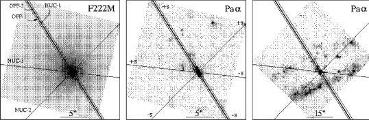
Figure 1: Slit positions overlayed, from left to right, on the F222M and $\mathrm{Pa}\alpha$ NICMOS 2 images (Schreier et al. 1998) and on the NICMOS 3 $\mathrm{Pa}\alpha$ image by Marconi et al. (2000). The ”NUC” and ”OFF” labels indicate the slit positions described in Table 1. ”s+” and ”s-” indicate the sign of the position along the slit used in the following figures. North is up and East is left.

Seeing during observations (performed in service mode) was in the range $0\farcs 4-0\farcs 6$, with photometric conditions. At a given position angle of the slit, the observation procedure was to obtain an acquisition image in K and then center the slit on the prominent nuclear peak (Paper I). For off nuclear positions a small telescope movement ($\pm 0\farcs 3$ perpendicular to the slit) was subsequently performed. After positioning the slit, observations consisted of several pairs of exposures in which the object was moved to two different positions along the slit (which we call A and B), in order to perform sky subtraction. This led to an effective slit length of 45″. The on-chip integration time was 180s resulting in a total on-source integration time of 36m at each slit position. The slit positions are summarized in Fig. 1 and the observation log is given in Tab. 1. The orientation of the NUC-1 slit was chosen to align with the major axis of the $\mathrm{Pa}\alpha$ disk. To give a clearer picture of any kinematical signature of the molecular bar, the NUC-2 slit was oriented along the bar major axis.

Data reduction was standard for near-ir spectroscopy and performed using IRAF. In each A or B frame, we first removed the electronic ghost using task is_ghost in the ESO ECLIPSE package (Devillard, 1997). The frames were then flat fielded with differential spectroscopic dome exposures and sky subtraction was performed for each couple of frames (A-B). Corrections for geometrical distortion of the slit direction and wavelength calibration were performed using OH sky line present on the detector (Oliva & Origlia, 1992). We verified that the rectification was performed to better than 0.1–0.2pix on the detector parts where the object is located ($\sim 300$pix along the slit). The relative accuracy of wavelength calibration was better than 0.2Å in K and J. After the 2 dimensional rectification procedure, we obtained two single spectra from each A-B frame and removed residual sky emission by fitting and subtracting a linear polynomium along the slit. Correction for the instrumental response and telluric absorption were performed by using the O6/O7 star HD113754, observed each night at the beginning and at the end of the observations. The intrinsic spectral shape of the standard star was removed by multiplying by $\lambda^{-4}$ which is typical of O5-9 stars in the near-ir.

The final 2d spectrum at each slit position was then obtained by averaging together all single frames. First, the frames were aligned along the slit via cross-correlation and shifts along the dispersion direction (due to grating movements between different instrument setups) where corrected using the OH sky lines present in each frame. With this correction the zero point of the wavelength scale has an accuracy of 0.4Å corresponding to a velocity error of 10$\,\mathrm{km}$$\,\mathrm{s}$^-1 in J and 6$\,\mathrm{km}$$\,\mathrm{s}$^-1 in K. All frames were then shifted to a common center and coadded rejecting bad pixels/cosmic rays.

We then selected the spectral regions containing the lines of interest and subtracted the continuum by a polynomial/spline fit pixel by pixel along the dispersion direction. The continuum subtracted lines were fitted, row by row, along the dispersion direction with Gaussian or Lorentzian functions using the task LONGSLIT in the TWODSPEC FIGARO package (Wilkins & Axon, 1992). When the SNR was insufficient (faint line) the fitting was improved by co-adding two or more pixels along the slit direction. All velocities where then corrected for Heliocentric motion. The results of this analysis are shown in the next section.

3 Results

3.1 Accuracy and stability of the slit position

Before analyzing the results of the observations, we discuss the accuracy of the target acquisition within the slit and the stability of the slit position during integration on source.

The target acquisition strategy consisted in centering the slit on the K band nuclear peak identified on the acquisition image. Given the strength of the K peak compared to the rest of the galaxy (cf. Paper I), the nucleus can be located accurately to better than a small fraction of the slit size ($<0\farcs 1$ given the seeing of the observations). A possible concern arises from observing in J following acquisition in K, if differential atmospheric refraction between J and K can move the nucleus out of the slit. We calculate, however, that in all cases differential atmospheric refraction can move the object less than 0$\farcs$05 perpendicular to the slit, and thus this effect is negligible.

The accuracy of the slit positioning is checked by comparing the rotation curves obtained at the same slit position in independent observations – the observations in J at NUC-1 and in K at OFF-2 were repeated. The comparison in shown in Fig. 2 for $\mathrm{Pa}\beta$ and $[\mathrm{Fe}\,\textsc{ii}]$ at NUC-1 and $\mathrm{H}_{2}$ at OFF-2. The filled squares are the repeated observations, with better seeing. It can be seen that the rotation curves are in agreement within the errors. Also, as expected, those obtained with worse seeing are smoother. The agreement shows that the procedure for target acquisition is quite accurate and that the offsets between repeated observations are much smaller than the slit size.

By comparing the 2d line maps obtained from single A/B frames, we also verified that any movement of the slit during observations does not significantly affect the rotation curves. In Fig. 3, we show the rotation curves obtained from $\mathrm{H}_{2}$ at NUC-1 from each A/B frame. This particular set of data represents the worst case: the continuum-subtracted position-velocity maps show the largest differences, indicating the greatest amount of slit movement during the observations. Allowing for lower signal-to-noise ratio with respect to the averaged map, all the A/B frames produce rotation curves which agree within the errors. The slit movements were not large enough to significantly affect the rotation curves, i.e. they were much smaller than the spatial resolution of the observations (0$\farcs$5).

3.2 Nuclear Spectra

The J and K averaged spectra extracted from $0\farcs 6\times 0\farcs 3$ apertures centered on the nucleus are presented in Fig. 4. The lines targeted for kinematical studies are $[\mathrm{Fe}\,\textsc{ii}]$ $\lambda$ 12566.8Å and $\mathrm{Pa}\beta$ $\lambda$ 12818.1Å, $\mathrm{H}_{2}$(1,0)S(1) $\lambda$ 21212.5Å and $\mathrm{Br}\gamma$ $\lambda$ 21655.3Å but we also detect other fainter $[\mathrm{Fe}\,\textsc{ii}]$ and $\mathrm{He}\,\textsc{i}$ lines. The strong K continuum (see Paper II for details) leads to a small equivalent width for $\mathrm{H}_{2}$ and $\mathrm{Br}\gamma$.

The nuclear spectrum is low excitation, indicated by the $[\mathrm{Fe}\,\textsc{ii}]/\mathrm{Pa}\beta\sim 1.7$ (e.g. Alonso-Herrero et al., 1997; Moorwood & Oliva, 1988). This ratio does not change with larger apertures which include more emission from the $\mathrm{Pa}\alpha$ disk detected in Paper I. Indeed, we showed in Paper II that the $[\mathrm{Fe}\,\textsc{ii}]$$\lambda$ 1.64$\,\mathrm{\mu m}$ and $\mathrm{Pa}\alpha$ morphologies are similar and that their ratio is constant over the disk.

The electron density of the emitting gas can be estimated using the ratio $[\mathrm{Fe}\,\textsc{ii}]$ $\lambda$ 12566.8Å/ $\lambda$ 12942.6Å $=0.15\pm 0.05$. Figure 5 displays the region in the $T_{\mathrm{e}}$-$N_{\mathrm{e}}$ plane allowed by the observed ratio. It indicates a density in the range 3.5–4.5$\,\mathrm{cm}$^-3 (in log), regardless of electron temperature. The $[\mathrm{Fe}\,\textsc{ii}]$ line ratio as a function of density and temperature was computed using a code kindly provided by E. Oliva which solves the detailed balance equations for a 16-level Fe⁺ ion, using atomic data from Zhang & Pradhan (1995). In Paper I we estimated the mass of the ionized gas disk assuming an electron density in the range $10^{2}$-$10^{4}$$\,\mathrm{cm}$^-3. The current measurement indicates a mass of ionized gas at the low end of the previous estimate, $\sim 10^{3}\mathrm{M}_{\odot}$.

An emission feature is clearly detected blueward of the brightest $[\mathrm{Fe}\,\textsc{ii}]$ line. Candidates for the identification are $[\mathrm{Fe}\,\textsc{ii}]$$\lambda$12521.3Å, $\mathrm{He}\,\textsc{i}$$\lambda$12527.4 ($3\,^{3}S-\,^{3}P^{o}$) or the high ionization coronal line $[\mathrm{S}\,\textsc{ix}]$$\lambda$12523.5Å (Oliva et al., 1994), as shown in the figure. All the lines (except for $[\mathrm{S}\,\textsc{ix}]$) are drawn at a redshift of $540\,\mathrm{km}\,\mathrm{s}^{-1}$, corresponding to the systemic velocity. Clearly, $\mathrm{He}\,\textsc{i}$ can be excluded since it would require a blue-shift of $\geq 240\,\mathrm{km}\,\mathrm{s}^{-1}$ which is not observed in other lines with similar excitation, like $[\mathrm{Fe}\,\textsc{ii}]$ and $\mathrm{Pa}\beta$. Moreover, none of the other $\mathrm{He}\,\textsc{i}$ lines expected in this spectral range are detected. $[\mathrm{Fe}\,\textsc{ii}]$$\lambda$12521.3Å can also be excluded since its ratio relative to $[\mathrm{Fe}\,\textsc{ii}]$$\lambda$12566.8Å for $N_{\mathrm{e}}=10^{4}\,\mathrm{cm}^{-3}$ is at most 0.01 while the observed feature would imply a ratio $\simeq 0.04$.

If the feature is indeed $[\mathrm{S}\,\textsc{ix}]$, it would require a blue-shift of $\simeq 150\,\mathrm{km}\,\mathrm{s}^{-1}$ with respect to the systemic velocity, as plotted in the figure. Indeed $[\mathrm{S}\,\textsc{ix}]$ has been detected in the Circinus galaxy (Oliva et al., 1994), NGC 1068 (Marconi et al., 1996) and has been found to be blue-shifted by $\simeq 40\,\mathrm{km}\,\mathrm{s}^{-1}$ and $\simeq 250\,\mathrm{km}\,\mathrm{s}^{-1}$, respectively (also cf. Oliva, 1997). Coronal lines blue-shifted with respect to lower excitation lines are often seen in other galaxies. Binette (1998) suggests that this is due to radiative acceleration of the coronal line clouds powered by the AGN continuum. Centaurus A has a very low excitation spectrum and it might be surprising to detect a high ionization coronal line (to produce the S VIII ion 351$\,\mathrm{eV}$ are required). However, when comparing data from similar slit sizes, the $[\mathrm{S}\,\textsc{ix}]$/$[\mathrm{Fe}\,\textsc{ii}]$ ratios in Circinus and NGC 1068 ($[\mathrm{S}\,\textsc{ix}]$/$[\mathrm{Fe}\,\textsc{ii}]$= 0.3 and 0.1, respectively) are much larger, by almost a factor 10, than in Cen A. The coronal line emission is usually spatially unresolved from the ground and concentrated at the nucleus; therefore large apertures strongly favor $[\mathrm{Fe}\,\textsc{ii}]$. Note that the spatial resolution and signal-to-noise ratio of the spectra presented here is almost unprecedented; spectra taken with previous instruments and smaller ground-based telescopes could not detect such faint lines.

Finally, we place an upper limit of $W_{\lambda}<5$Å to the equivalent width of any broad ($>1000\,\mathrm{km}\,\mathrm{s}^{-1}$) $\mathrm{Pa}\beta$ component.

3.3 Gas kinematics

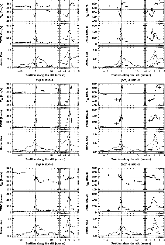
Figure 6: Heliocentric velocities ($\,\mathrm{km}$$\,\mathrm{s}$^-1), FWHM ($\,\mathrm{km}$$\,\mathrm{s}$^-1) and fluxes (arbitrary units) plotted as a function of the position along the slit (arcsec) for $\mathrm{Pa}\beta$ and $[\mathrm{Fe}\,\textsc{ii}]$. The dotted lines are drawn for $s=0$ and $V_{\mathrm{Hel}}=535\,\mathrm{km}\,\mathrm{s}^{-1}$. The dashed lines in the ”flux” panels represent the continuum flux along the slit.

Heliocentric velocities, FWHM (Full Width at Half Maximum) and fluxes measured along each of the slits are shown in Fig. 6, 7 and 8. The corresponding slit positions are described in Table 1 and shown in Fig. 1. In the rest of the paper, we will refer to $s$ as the coordinate describing the position along the slit. In $K$ the zero point of $s$ is defined by the position of the near-IR peak which marks the nucleus of the galaxy (Paper I and II). In $J$ the zero point is also located by fitting the rotation curve. The $+$ or $-$ sign of $s$ is also indicated in Fig. 1 to help associate velocities with locations in the galaxy.

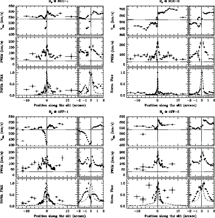
Figure 8: $\mathrm{H}_{2}$ plots (same notation and layout as in Fig. 6).

The ionized gas rotation curves can be decomposed into two distinct velocity systems. The first is an extended component ($|s|>2\arcsec$), characterized by small velocity gradients and a FWHM close to the instrumental resolution (30$\,\mathrm{km}$$\,\mathrm{s}$^-1 in J and 33$\,\mathrm{km}$$\,\mathrm{s}$^-1 in K). The second velocity system is confined within the central $|s|<2\arcsec$ and is characterized by large velocity amplitudes and gradients, FWHMs which rise sharply close to $s=0$ and peak at $\sim 600\,\mathrm{km}\,\mathrm{s}^{-1}$, and by a flux much larger than that of the extended region. We refer to this as the nuclear component. These components can be traced also in the molecular gas but, in addition, a further extended kinematical component is seen in $\mathrm{H}_{2}$ at NUC-2, as shown in Fig. 8 and 9; this component is not present in the ionized gas.

3.3.1 The extended component

The velocity field of the extended component of the ionized gas (cf. at all three slit positions of the $\mathrm{Pa}\beta$ data) has small gradients and a quite regular structure which can be followed out to $\sim 15\arcsec$ from the nucleus.

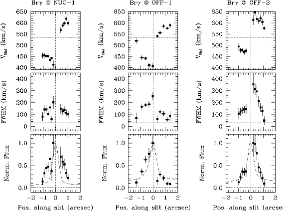
Figure 7: $\mathrm{Br}\gamma$ plots in the inner 2″ (same notation as in Fig. 6).

Our data can be compared with the analysis by NBT92 performed using optical lines. Their data, covering most of the dust lane, are well accounted for by a model in which the gas is distributed in an optically thin warped disk. Using the full two dimensional information, NBT92 determined the kinematic line of nodes for this ionized gas disk which is found to bend, following the warping of the dust lane. In the inner 15″ (the region covered by our data) the kinematic line of nodes has a PA $\sim 90^{\circ}$. This is consistent with the fact that the velocity gradient in our data increases from PA $33^{\circ}$ to PA $-45^{\circ}$, reaching a maximum value of 4$\,\mathrm{km}$$\,\mathrm{s}$^-1/arcsec at PA $84^{\circ}$. This value agrees well with the $\sim 3.7\,\mathrm{km}\,\mathrm{s}^{-1}$/arcsec that we derive from Fig. 7 of NBT92. At the distance of Cen A (3.5Mpc), it corresponds to 235 $\,\mathrm{km}$$\,\mathrm{s}$^-1$\,\mathrm{kpc}$^-1. Note that, NBT92 did not find high velocity gas or line widths larger than 40$\,\mathrm{km}$$\,\mathrm{s}$^-1 at the nucleus of Cen A. This is very likely due to reddening within the inner 2″  where any nuclear $\mathrm{H}\alpha$+$[\mathrm{N}\,\textsc{ii}]$ emission can be completely hidden ($A_{\mathrm{V}}>5$mag, see Paper II).

The kinematics of the extended gas component can also be studied from the molecular gas as traced by the $\mathrm{H}_{2}$ line. While at NUC-1 the $\mathrm{Pa}\beta$ and $\mathrm{H}_{2}$ velocity curves are very similar, at NUC-2, the $\mathrm{H}_{2}$ velocity shows a sharp linear rise between $3\arcsec<s<6\arcsec$, with a peak to peak amplitude of $\sim 300\,\mathrm{km}\,\mathrm{s}^{-1}$ at $\pm 6\arcsec$, and then a smooth decrease out to $10\arcsec$ where the velocity drops to its systemic value. It traces the kinematics of the molecular gas alone, as it is not observed in $\mathrm{Pa}\beta$ and $[\mathrm{Fe}\,\textsc{ii}]$. This velocity structure is symmetric with respect to the zero point (i.e. $V=V_{sys}$ and $s=0$) and is suggestive of the rotation curve of a ring, with an inner ”solid body rotation” and an outer keplerian decrease. The origin of this kinematical feature will be discussed in Section 5.3.

3.3.2 The nuclear component

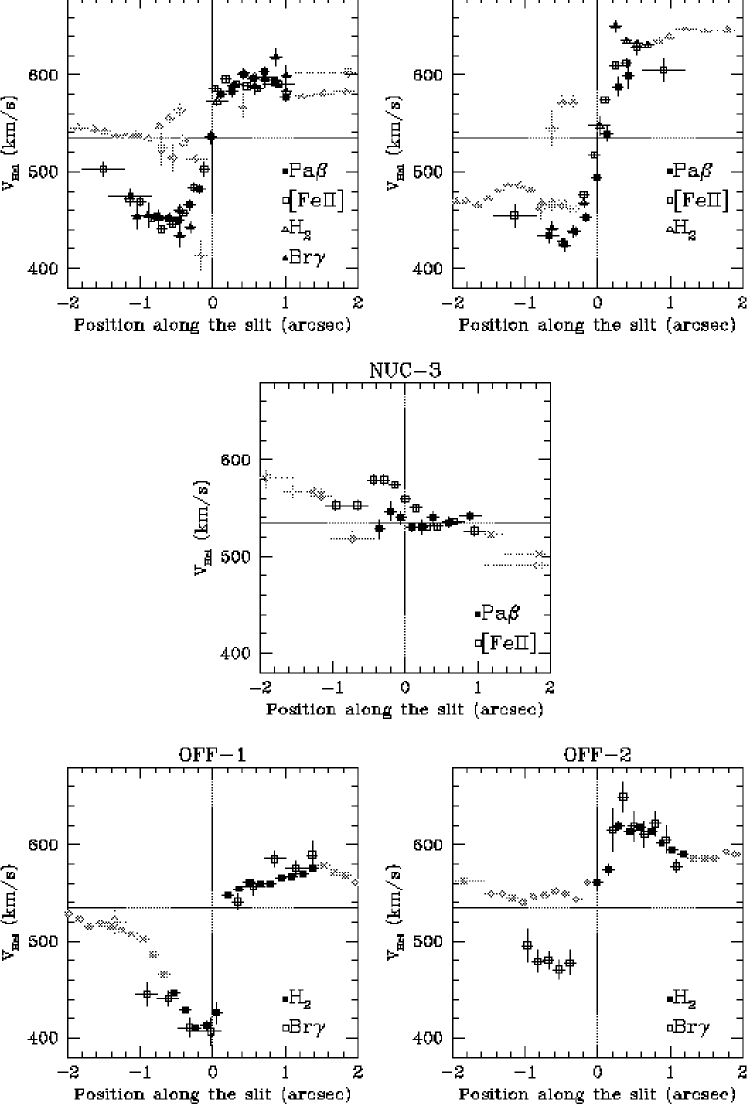
Figure 10: Comparison of velocities in the inner 2″. The grey color marks the points ”contaminated” by the extended component which are not used in the fit.

At the positions NUC-1 and 2, the ionized gas shows a well defined S-shaped velocity curve with peak to peak amplitudes up to $\sim 200\,\mathrm{km}\,\mathrm{s}^{-1}$. Velocities from different lines in the inner 2″ are compared in Fig. 10. The $\mathrm{Pa}\beta$, $[\mathrm{Fe}\,\textsc{ii}]$ and $\mathrm{Br}\gamma$ data agree remarkably well at all slit positions. There is a region of small discrepancy at 0$\farcs$5 seen in the NUC-2 spectrum probably caused by contamination from the extended component as discussed below. The $\mathrm{Br}\gamma$ equivalent width drops dramatically within the central 0$\farcs$5 due to the strong nuclear continuum making velocity measurements impossible with the present data.

These velocity curves are strongly suggestive of gas rotation within a thin disk. This interpretation is supported by comparing the velocity curves at position angles 33°and -45° with that at PA 84°. The latter has a very small amplitude as expected if that position angle for the slit is almost perpendicular to the line of nodes of the disk which, therefore, should be oriented close to North-South. At all positions, we find a sharp increase in FWHM near the nucleus, the expected consequence of unresolved rotation close to the nucleus: it is not possible to trace the rotation curve within a spatial resolution element from the nucleus, and the mixing of high velocity components broadens the line profile. We will return to this in Sec. 4.1.

The $\mathrm{H}_{2}$ rotation curves in the inner 2″ are also compared with those of the ionized gas in Fig. 10. The amplitude of the $\mathrm{H}_{2}$ rotation curve, particularly at NUC-1, is smaller than those of $\mathrm{Pa}\beta$, $[\mathrm{Fe}\,\textsc{ii}]$ and $\mathrm{Br}\gamma$. Note, however, the double $\mathrm{H}_{2}$ line profiles between $-1\arcsec<s<-0\farcs 4$ (Fig. 11). When accurate deblending is possible, the blueshifted velocity component agrees with the velocities measured from the ionized gas (Fig. 10). In the adjacent points, where deblending is impossible, the width of the lines is larger ($\sim 100\,\mathrm{km}\,\mathrm{s}$) and the measured velocity is an intensity weighted average of the two components. The ”contamination” from the extended component is particularly evident for $s<0\arcsec$, i.e. south of the nucleus (cf. Fig. 1), at NUC-1 and OFF-2. It is also responsible for the sharp decrease in $\mathrm{H}_{2}$ velocity observed at OFF-1 below $-0\farcs 6$. The discrepant $[\mathrm{Fe}\,\textsc{ii}]$ velocities at NUC-2 are also likely caused by mixing of these 2 velocity components and the increased $[\mathrm{Fe}\,\textsc{ii}]$ line widths at this location support this interpretation.

The high velocity components are thus present also in the molecular lines but they are partly hidden by the superposition with the extended component. However, when deblending is possible, velocities from the rotating disk can still be measured and they are in agreement with those from the ionized gas. This ”contamination” is likely to be present also in the other lines but their extended components are much weaker with respect to the nuclear ones (see the line fluxes along the slit in the figures) and do not affect the velocity determination in the inner 2″.

4 Kinematical Models of the nuclear rotation curves

The nuclear velocity curves described in the previous section clearly suggest gas rotating in a disk around a compact mass. We now investigate if they are indeed quantitatively consistent with this interpretation. Under the hypothesis of a thin gaseous disk circularly rotating in the gravitational potential of a point mass $M$, the rotation curve at a given slit position can be written as (Macchetto et al., 1997)

$$V=V_{sys}-(GM)^{0.5}\sin i\frac{X}{R^{1.5}}$$ (1)

where $R$ is the deprojected radial distance, $X$ is the distance from the disk minor axis and $i$ is the disk inclination with respect to the line of sight ($i=0$ is the face-on case). The geometry and definitions are also summarized in Fig. 19 and in the Appendix.

This formula provides the velocity along a thin slit but is not immediately applicable since the finite spatial resolution of the observations smears the velocity cusps of the rotation curve. Moreover, the measured velocities are intensity weighted averages over apertures determined by the slit size and the number of pixels integrated along the slit. To simulate the effects of seeing, we convolve with a gaussian PSF (Point Spread Function) with FWHM equal to the seeing of the observations ($0\farcs 5$). We then integrate over the slit size to derive the expected velocity $V_{psf}$ as a function of the slit coordinate $s$.

The observations provide us with several datasets, each from a given line ($\mathrm{Pa}\beta$, $[\mathrm{Fe}\,\textsc{ii}]$  $\mathrm{H}_{2}$ or $\mathrm{Br}\gamma$) at a given slit position (NUC-1, NUC-2, NUC-3, OFF-1 and OFF-2). Each data set $k$ comprises $n_{k}$ points and each point is characterized by its position along the slit $x_{i}$ (in pixels, i.e. detector coordinates) and its velocity $V_{i}$ (in $\,\mathrm{km}$$\,\mathrm{s}$^-1) derived from the line fitting procedure. Three free parameters are associated with each dataset:

• $x_{0k}$, the pixel at which $s=0$;

• $b$_k, the distance of the center of the slit from the nucleus;

• $\theta$_k, the angle between the slit and the line of nodes of the disk;

$x_{0k}$ is fixed at the position of the continuum peak. In the K band, the continuum peak undoubtedly identifies the location of the nucleus, given its strength relative to the surrounding emission from the galaxy. In the J band, however, the continuum peak has an intensity comparable with that of the extended emission: any asymmetry in the galaxy emission (due, e.g., to an extinction gradient) could shift the peak of the continuum with respect to the position of the nucleus. Therefore $x_{0}$_k must be allowed to vary with respect to the position of the flux peak by the same amount for lines from the same spectrum. Once $x_{0k}$ and the pixel size are set, the coordinate $s$ along the slit is given by $s_{i}=0\farcs 147\times(x_{i}-x_{0k})$.

For the nuclear positions NUC-1,2 and 3, $b$_k is set to 0, given that the acquisition procedure and the telescope guiding accuracy is well below 0$\farcs$1. For the off-nuclear position, $b$${}_{k}=\pm 0\farcs 3$.

Since the relative orientation of each pair of slit positions is fixed by the observational strategy, all values of $\theta_{k}$ are determined by a single value $\theta$, the angle between the line of nodes and the North-South direction.

The ”global” free parameters are:

• $i$, the inclination of the disk;

• $M_{\bullet}$, the black hole mass;

• $V_{\mathrm{Sys}}$, the systemic velocity.

We fit the free parameters by minimizing $\chi_{\mathrm{Red}}^{2}$:

$$\chi_{\mathrm{Red}}^{2}=\frac{1}{\sum_{k=1}^{N}n_{k}-f}\sum_{k=1}^{N}\sum_{j=1}^{n_{k}}\frac{\left(V_{j}-V_{psf}(x_{j};x_{0k},\theta,i,M_{\bullet},V_{\mathrm{Sys}})\right)^{2}}{\Delta V_{j}^{2}}$$ (2)

where N is the total number of datasets and $f$ is the number of free parameters.

Since, as shown in the previous section, the $\mathrm{H}_{2}$ rotation curves of the nuclear component are contaminated by the extended component, and the signal-to-noise and spatial sampling of the $\mathrm{Br}\gamma$ data is poorer than that of $[\mathrm{Fe}\,\textsc{ii}]$ and $\mathrm{Pa}\beta$, we fit only the latter two lines. The $\mathrm{H}_{2}$ and $\mathrm{Br}\gamma$ data are used only as a consistency check after performing the fit. The velocity points excluded from the fit are drawn in grey color in Fig. 10.

The best fits for fixed values of the disk inclination are shown in Figs. 12 and 13; the resulting parameters are given in Tab. 2. The agreement between the data and the models is good for all three slit positions at disk inclinations below 60°. The residuals do not show any systematic trend and their rms is typically $\sim 10$ $\,\mathrm{km}$$\,\mathrm{s}$^-1.

Although the best fit models trace the data well, the minimum $\chi_{\mathrm{Red}}^{2}$ values are far larger than expected for a good fit. This discrepancy probably arises from the fitted data points not being statistically independent. From a visual inspection of the fits, we estimate typical uncertainties on fit parameters as $\Delta\theta\pm 5\arcdeg$, $\Delta V_{\mathrm{Sys}}\pm 5\,\mathrm{km}\,\mathrm{s}^{-1}$, and $\Delta M_{\bullet}/M_{\bullet}\pm 20\%$.

We assess the validity of our results by comparing the model rotation curves with the observed $\mathrm{H}_{2}$ and $\mathrm{Br}\gamma$ curves (see Fig. 14). In particular, the asymmetric behaviour of the off-nuclear rotation curves measured from the $\mathrm{H}_{2}$ and $\mathrm{Br}\gamma$ lines, typical of the impact parameter being not zero, is naturally accounted for.

We examined the effects of varying the disk inclination on the determination of the value of the central mass; these two parameters are strongly coupled, since the amplitude of the rotation curve is proportional to $M_{\bullet}^{0.5}(\sin i)$. A weaker dependence on $i$ alone is also present, as the deprojected radius $R$ depends on $\cos i$ (see the Appendix). We find that the signal-to-noise of our data is sufficient to reject all values of $i$ ($>60\arcdeg$), since the model is not able to reproduce the observed velocity amplitude at NUC-1 and NUC-2 at the same time. For such large values of inclination, varying the angle with the disk line of nodes maps very different radial distances $R$ into similar slit coordinates $s$, thus requiring different masses to reproduce a given velocity. Conversely, all values of inclination $i\lesssim 60\arcdeg$ produce acceptable fits. The minimum dynamical mass required by the data is $\sim 9\times 10^{7}\mathrm{M}_{\odot}$; this estimate obviously increases with decreasing disk inclination.

It is clear from inspection of Tab. 2 that regardless of inclination, the systemic velocity is well determined at $V_{\mathrm{Sys}}=532\pm 5\,\mathrm{km}\,\mathrm{s}^{-1}$, in agreement with published values. Similarly, the position angle of the line of nodes is well constrained, in the range $-10\arcdeg\div-14\arcdeg$. Note that the kinematic line of nodes (PA=-14°) determined from our velocity curves differs from the axis of elongation of the $\mathrm{Pa}\alpha$ disk (PA=33°) seen with NICMOS. This can be explained if only a part of the disk is ionized and lies within the ionization cone (the jet axis projected on the sky has PA $\simeq 55\arcdeg$); the ionized portion is then visible in $\mathrm{Pa}\beta$ and $[\mathrm{Fe}\,\textsc{ii}]$. Another possibility is that the disk density, and thus the emission measure, is very low outside of the region observed with NICMOS in $\mathrm{Pa}\alpha$.

4.1 The nuclear line profiles

The line flux profile along the slit in the inner $|s|<0\farcs 5$ is strongly peaked and unresolved; its FWHM is comparable to the seeing ($\sim 0\farcs 5$) and is the same regardless of slit orientation. We conclude that the line luminosity profile along the slit has a FWHM less than 0$\farcs$1; otherwise it would appear spatially resolved. The actual surface brightness distribution of the line around the nucleus is unknown. If we assume a double exponential profile extending down to a minimum radius $r_{h}$

$$I(r)=\left\{\begin{array}[]{ll}I_{0}\,\mbox{e}^{-\frac{r}{r_{0}}}+I_{1}\,\mbox{e}^{-\frac{r}{r_{1}}}&r\geq r_{h}\\ 0&r<r_{h}\end{array}\right.$$ (3)

where $r_{0}$ and $r_{1}$ are the scale radii, the values $r_{0}=0\farcs 08$, $r_{1}=1\arcsec$, $r_{h}=0\farcs 08$ and $I_{1}/I_{0}=0.015$ match the line flux distributions along the slit.

Performing the fit with an intensity profile does not significantly changes the results as shown in Tab. 2 and parameters relative uncertainties are also the same as before. A fit example is shown in Fig. 15. All the parameters agree within uncertainties with the estimates performed with a constant surface brightness. The only significant difference is a slightly worse value of $\chi_{\mathrm{Red}}^{2}$. Note that, though within the 20% uncertainty, the masses are slightly lower than in the case with constant light distribution. The reason is that the adopted light distribution places more weighting to the points closer to the nucleus and a given velocity amplitude can be reproduced with a smaller mass. However, we have also verified that surface brightness distributions which are strongly peaked toward the center are excluded because they give too much weight to the high velocity components. This explains why a ”hole” in line emission around the nucleus is required.

With this assumption on the surface brightness line distribution, we compute the line profiles expected from a rotating disk and compare them with the observed ones. The detailed formula is given in the appendix. Assuming pure gravitational motion of the gas, differing line profiles are the consequence of unresolved rotation in the inner parts. Therefore, a crucial test for the keplerian rotation assumption is verifying that the observed line widths are consistent with unresolved rotation and not the result of non-gravitational motions.

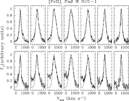
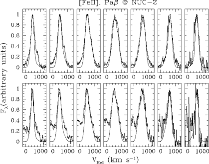
Figure 16: Expected line profiles obtained from a disk in keplerian rotation around a point mass compared with the observed ones. The inclination of the disk is $i$=45°, the surface brightness line distribution is a double exponential (see Table 2 for the values of the model parameters).

In Figure 16, we compare the model profiles with the observations. We have assumed intrinsic gaussian line profiles, with FWHM increasing linearly from 50$\,\mathrm{km}$$\,\mathrm{s}$^-1 at 1″ from the nucleus to 250$\,\mathrm{km}$$\,\mathrm{s}$^-1 at 0$\farcs$1. The line profiles are computed for $i$=45° with the corresponding parameters as in Table 2. There is reasonable agreement between the model profiles and the observed data which could be improved further by optimizing the intrinsic FWHM of the line profiles. In Sec. 3.1 we showed that the slit positioning was stable during the observations by comparing rotation curves obtained from independent observations. Though a small movement of the slit does not produce any appreciable change in the line centroid, it can change the line profiles. Therefore, some differences between model and observed line profiles can be accounted for by small movements of the slit. Another point to be considered is the dependence of the line profiles on the assumed surface brightness distribution. The most important point is that at all slit positions, unresolved rotation can fully account for the observed FWHM of the lines and we can reproduce the observed line profiles. A more detailed analysis of this kind requires higher spatial resolution. Planned HST observations should be characterized by higher resolution and better stability in slit positioning.

4.2 Stellar contribution to the dynamical mass

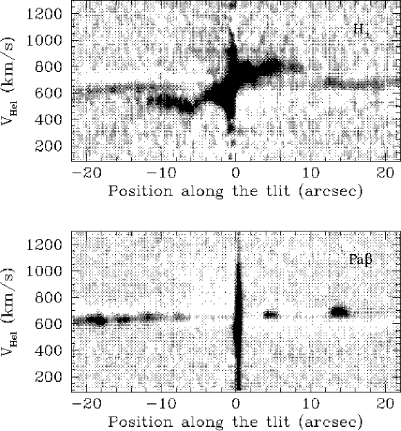
Figure 9: Grey scales of $\mathrm{H}_{2}$ and $\mathrm{Pa}\beta$ position-velocity diagrams at NUC-2.

The observed rotation curves require a mass of $M_{\bullet}>6\times 10^{7}\mathrm{M}_{\odot}$ within $R<0\farcs 25$, as set by the spatial resolution of our observations. It is crucial to determine if this large mass can be accounted for by stars. In Paper II, we reconstructed the nuclear light profile in the V band (assuming a color-based reddening correction and no color gradients in V-K and V-H) and showed that it can be well fitted with a Nuker law with a break occurring at $r_{b}\sim 4\arcsec$ (see Fig. 9 in Paper II and Fig. 18a). For the inner $R<10\arcsec$, we used the NICMOS F222M image whose isophotes (after reddening correction) are characterized by small ellipticities ($<0.1$) and are therefore consistent with a spherical stellar system. When a system is characterized by a spherical light density ${\cal J}(R)$ the observed surface brightness is given by

$$\Sigma(r)=2\int_{r}^{+\infty}\frac{{\cal J}(R)RdR}{\sqrt{R^{2}-r^{2}}}$$ (4)

where $r$ is the projected radius onto the plane of the sky and $R$ is the distance from the nucleus. Once $\Sigma(r)$ is obtained from observation, the above equation can be inverted to derive ${\cal J}(R)$ using Abel’s formula:

$${\cal J}(R)=-\frac{1}{\pi}\int_{R}^{+\infty}\frac{d\Sigma(r)}{dr}\frac{dr}{\sqrt{r^{2}-R^{2}}}$$ (5)

The mass density is then given by $\rho(R)=4\pi\,\Upsilon{\cal J}(R)$ where $\Upsilon$ is the mass-to-light ratio, and the mass enclosed within the radius $R$ can be computed. In Fig. 18a, we plot the reddening corrected K band surface brightness points along with the best fit nuker-law profile presented in Paper II (solid line). The dashed line represents the nuker law with the steepest profile consistent with the data. In Fig. 18b we show the derived luminosity density ($\mathrm{L}_{\mathrm{K}\odot}$ is the solar luminosity in the K band) and, finally, in Fig. 18c, we show the enclosed mass within a given radius $R$ for a Mass-To-Light ratio, $\Upsilon=1\mathrm{M}_{\odot}/\mathrm{L}_{\mathrm{K}\odot}$. Note that the steepness of the nuclear cusp is fundamental to estimating the enclosed mass at small radii.

Within $R=0\farcs 25$, the scale probed by our observations, the Mass-to-Light ratio required to account for the rotation curve of the ionized disk is $>20\mathrm{M}_{\odot}/\mathrm{L}_{\mathrm{K}\odot}$ ($>6\mathrm{M}_{\odot}/\mathrm{L}_{\mathrm{K}\odot}$ with the steepest nuclear cusp consistent with the data). The observed mass-to-light ratio of elliptical galaxies with total mass around $10^{11}$$\mathrm{M}_{\odot}$ lies in the range $\Upsilon=0.15-0.5\mathrm{M}_{\odot}/\mathrm{L}_{\mathrm{K}\odot}$ (Mobasher et al., 1999) and in bulges of early type spiral galaxies is typically $\Upsilon\simeq 0.6\mathrm{M}_{\odot}/\mathrm{L}_{\mathrm{K}\odot}$ (Moriondo, Giovanardi & Hunt, 1998). According to stellar population synthesis models, mass-to-light ratios up to $\Upsilon\sim 1.3$ at $t=15$ Gyr can be obtained with a Salpeter Initial Mass Function (Maraston, 1998). Though with a very steep IMF the stellar population can reach $\Upsilon\simeq 4\mathrm{M}_{\odot}/\mathrm{L}_{\mathrm{K}\odot}$ after 15 Gyr, it is clear that the mass-to-light ratio required by our observations is incompatible with a ”normal” stellar system and suggests the presence of a dark mass concentration.

The central mass density is $\simeq 3\times 10^{5}M_{8}\,\mathrm{M}_{\odot}\,\mathrm{pc}^{-3}$ ($M_{8}$ is the mass in units of $10^{8}$$\mathrm{M}_{\odot}$) and similarly high mass densities have been observed in a few core-collapsed globular clusters (Pryor & Meylan, 1993). We therefore cannot strictly rule out that the central dark mass concentration is an ”exotic” object such as a massive cluster of neutron stars or other dark objects; an extensive discussion of such possibilities has been given by van der Marel et al. (1997). However we concur with their general conclusion that these alternatives are both implausible and contrived. We believe that the more conservative explanation for the central mass concentration observed in Centaurus A is indeed a supermassive black-hole.

To summarize, the observed stellar light profile cannot explain the observed rotation curves for any reasonable choice of M/L, leading us to conclude that a dark mass of $M_{\bullet}>6\times 10^{7}\mathrm{M}_{\odot}$ is required. The lower limit for the Black Hole mass in Cen A is directly constrained by the observed rotation curves, but the upper bound is essentially unconstrained (e.g., for $i=5\arcdeg$, we would obtain a mass value two orders of magnitude larger). Nonetheless, a very small inclination can be reasonably excluded by the properties of the radio jet in Cen A, whose direction is thought to be very close to the plane of the sky. From VLBI observations, Tingay et al. (1998) derived a value for jet inclination with respect to the line of sight of 50°–80°. Near-IR polarimetry of Cen A with NICMOS (Capetti et al., 2000) indicates that emission from the nucleus escapes within a light cone, visible in polarized light. This is possible only if the the line of sight is outside the cone, whose axis must then be close to the plane of the sky. Although there might be a misalignment between the jet and the ionized disk, it appears very unlikely that a jet in the plane of the sky could be associated with a face-on disk. Excluding only the smallest disk inclinations ($i<15\arcdeg$), an upper limit on the BH mass can be set at $M_{\bullet}=5\times 10^{8}\mathrm{M}_{\odot}$. We conclude that the black hole mass estimate is $M_{\bullet}=2^{+3.0}_{-1.4}\times 10^{8}\mathrm{M}_{\odot}$.

5 Discussion

The observations presented above provide strong evidence for a dark mass concentration, very likely a supermassive black hole, at the nucleus of Cen A. The BH sphere of influence has an outer radius

$$r_{\bullet}\simeq\frac{GM_{\bullet}}{\sigma^{2}}=11\,\mathrm{pc}\left(\frac{M_{\bullet}}{10^{8}\mathrm{M}_{\odot}}\right)\left(\frac{\sigma}{200\,\mathrm{km}\,\mathrm{s}^{-1}}\right)^{-2}$$ (6)

where $G$ is the gravitational constant and $\sigma$ is the velocity dispersion of the stars. In Cen A, the velocity dispersion has a mean value of $\simeq 120\,\mathrm{km}\,\mathrm{s}^{-1}$ between 40″ and 80″ from the centre with a nuclear value of $\sim 150\,\mathrm{km}\,\mathrm{s}^{-1}$ (Wilkinson et al., 1986). With the caveat that extinction could lead to an underestimate of the nuclear value, the radius of influence of the BH would then be $r_{\bullet}\sim 20M_{8}\,\mathrm{pc}$ i.e. $\sim 1.1\arcsec M_{8}$. Indeed the nuclear rotation curves within 2″ of the nucleus do not show any evidence of an extended mass distribution. The radius of influence of the BH could also be estimated as the radius where the enclosed stellar mass equals $M_{\bullet}$. From Fig. 18c, for $\Upsilon=1\mathrm{M}_{\odot}/\mathrm{L}_{\mathrm{K}\odot}$ this takes place at $R\sim 1\arcsec$, or 17pc, (for $M_{\bullet}$=$10^{8}$$\mathrm{M}_{\odot}$), consistent with the above estimate.

The presence of a supermassive BH at the nucleus of Cen A has implications for the energetics of the active nucleus and for the general BH-mass vs bulge-mass relationship.

5.1 BH mass and AGN activity

In the 2-10$\,\mathrm{keV}$ range, the nucleus of Centaurus A has an unabsorbed X-ray luminosity of 6$\times 10^{41}$$\,\mathrm{erg}$$\,\mathrm{s}$^-1  with a power law spectrum typical of normal AGNs - $\Gamma=1.96\pm 0.1$ (Turner et al., 1997). For a typical quasar, $L_{X}(2-10\,\mathrm{keV})/L_{\mathrm{bol}}\sim 0.03$ (Elvis et al., 1994); assuming that Cen A has a similar Spectral Energy Distribution (SED), its expected bolometric luminosity is $\simeq 2\times 10^{43}\,\mathrm{erg}\,\mathrm{s}^{-1}$, in agreement with other estimates presented in literature (e.g. Kinzer et al., 1995). This value indicates that Cen A is radiating well below its Eddington luminosity as $L_{\mathrm{bol}}/L_{Edd}\simeq 2.4\times 10^{-3}M_{8}^{-1}$, where $M_{8}^{-1}$ is the BH mass in units of $10^{8}$$\mathrm{M}_{\odot}$. This is similar to the case of M87, another well-studied radio galaxy characterized by a prominent jet and a supermassive BH (c.f. Macchetto et al., 1997). The HST survey of nuclei of FR I radio-galaxies by Chiaberge, Capetti & Celotti (1999) indicates that sub-Eddington luminosities are typical of this class of sources to which Cen A belongs.

Luminosities much below the Eddington limit are the result either of a very low accretion rate or of an inefficient radiation process. In the latter case it has been suggested that the accretion is dominated by advection (Advection Dominated Accretion Flow - ADAF; e.g. Narayan, Kato & Honma, 1997) in which case the continuum emitted by the AGN lacks the UV ”big-blue bump” emitted by the standard thin accretion disk (e.g. Kurpiewski & Jaroszynski, 2000; Di Matteo et al., 2000).

Using ISO LWS spectra, Unger, Clegg & Stacey (2000) have shown that the total FIR luminosity of Cen A in a 70″ beam centered on the nucleus is $L_{\mathrm{FIR}}=3.2\times 10^{9}\mathrm{L}_{\odot}$, comparable to the luminosity expected from the AGN, $L_{\mathrm{AGN}}\simeq 5\times 10^{9}\mathrm{L}_{\odot}$, if it has the typical spectrum of a quasar. If the latter assumption is true, the sub-Eddington luminosities are the consequence of a low accretion rate. However, since FIR emission lines have excitation and equivalent widths typical of starburst galaxies, Unger, Clegg & Stacey (2000) suggest that the total FIR luminosity of Cen A is dominated by star formation instead of AGN activity. In this case the bolometric correction applied to the AGN X-ray emission is overestimated by a large factor (a factor of 10 would imply $L_{\mathrm{AGN}}/L_{\mathrm{FIR}}\simeq 0.15$) suggesting that the big blue bump is weak or absent as it happens in the ADAF regime. Indeed, in Paper II we showed that the extrapolation of the X-ray power law to the optical and near IR can fully account for the observed nuclear emission.

5.2 The BH-mass vs bulge-mass relationship

There is increasing evidence that black holes exist in most or all galaxies, and it has been suggested that a rough correlation exists between the mass of the black hole and the mass of the bulge of the host galaxy (e.g. Kormendy & Richstone, 1995; Richstone et al., 1998). In this framework, we can compare the central dark mass concentration in Cen A with the total mass of the galaxy.

The total mass of Cen A has been derived by photometrical and kinematical studies. Hui et al. (1993) and Mathieu & Dejonghe (1999) find $M_{\mathrm{sph}}=(4\pm 1)\times 10^{11}\mathrm{M}_{\odot}$. However, in the BH-bulge mass relationships, the spheroid mass is usually determined by assuming a mass-to-light ratio from the spheroid luminosity in a certain band (usually V or B). To compare Cen A with existing BH-bulge relationships, we thus have to verify that the photometry results are compatible with the kinematics. Indeed, the total V mag of Cen A is V=5.75mag (from Dufour et al. (1979), after correcting for the nuclear light profile - Paper II), which corresponds to $M_{\mathrm{V}}$=-21.95mag. Therefore $\log(L/\mathrm{L}_{\mathrm{V}\odot})=0.4(-M_{\mathrm{V}}+4.83)=10.7$. For normal galaxies, $M/L_{\mathrm{V}}=5(L/10^{10}\mathrm{L}_{\mathrm{V}\odot})^{0.2}$ in solar units, and therefore the expected mass of Cen A is $M\sim 3\times 10^{11}\mathrm{M}_{\odot}$ in good agreement with the kinematical determination.

For Cen A, then:

$$\frac{M_{\bullet}}{M_{\mathrm{sph}}}\simeq 2.5\times 10^{-4}M_{8}$$ (7)

where $M_{8}$ is the BH mass in units of $10^{8}$$\mathrm{M}_{\odot}$. The well known BH-mass vs bulge-mass relationship (Richstone et al., 1998) shows that $\log(M_{\bullet}/M_{\mathrm{sph}})$ has a roughly gaussian distribution, with an average of -2.27 (i.e. a 0.005 ratio) and standard deviation of 0.5. The expected relationship from Quasar light is $\simeq 6\times 10^{-4}$, a factor ten lower. This apparent discrepancy suggests that AGN accretion is less efficient than previously thought or that most of AGN activity is obscured (Fabian & Iwasawa, 1999). Note however that the large observed value of 0.005 is based on the Magorrian et al. (1998) paper where, given the simplified assumptions on the stellar systems and the low spatial resolution of the spectroscopic data, BH masses are likely overestimated. Indeed Cen A is almost 2.5$\sigma$ (in log) below the average of the Richstone et al. and Magorrian et al. papers while it is in good agreement with the expectation from Quasar light. The observed $M_{\bullet}/M_{\mathrm{sph}}$ for Cen A is also in agreement with the same ratio determined by Wandel (1999) for Seyfert 1 galaxies from reverberation mapping.

5.3 The $\mathrm{H}_{2}$ ”ring”

We have showed that while the $\mathrm{H}_{2}$ rotation curve well fits our picture of a fast rotating disk around a SMBH within the central 2″, at larger radii the $\mathrm{H}_{2}$ velocities at NUC-2 are very different from those of the ionized gas. From the inspection of Fig. 9, the large scale velocity structure of the $\mathrm{H}_{2}$ shows two distinct velocity components. One has a constant velocity gradient and corresponds to the extended rotating structure also seen in the ionized gas. The second velocity component, only seen in $\mathrm{H}_{2}$ between 2″ and 10″, is reminiscent of a rotating ring with an inner radius of 6″ and a keplerian fall-off. Fig. 8 shows that the $\mathrm{H}_{2}$ flux at NUC-1 within 2″ has two secondary maxima at $\simeq 1\arcsec$ on both sides from the nucleus, as expected from a circumnuclear ring. The same two maxima, however, are not observed at NUC-2. Comparing the projected radius at NUC-1 and the kinematical inner radius at NUC-2, the ”ring” must be almost edge-on ($i>80\arcdeg$), in agreement with the absence of the high velocity $\mathrm{H}_{2}$ components at NUC-1, OFF-1 and OFF-2 where the slit PA is perpendicular.

In summary, this putative molecular ”ring” has an inner radius of $\simeq 100\,\mathrm{pc}$, is almost edge on ($i>80\arcdeg$) and, from the velocity amplitude, includes a mass $M=0.6-2.5\times 10^{9}\mathrm{M}_{\odot}$. The uncertainty on the mass derives from the uncertainties on the inclination and the inner radius of ring.

This high velocity component is the $\mathrm{H}_{2}$ counterpart of the 100$\,\mathrm{pc}$-scale molecular ring previously identified by several authors in CO and FIR (Israel et al., 1990, 1991; Rydbeck et al., 1993; Hawarden et al., 1986). In CO, its major axis is oriented perpendicularly to the jet at PA$\sim 145\arcdeg$, its radius ranges between 80 and 140$\,\mathrm{pc}$ and its rotational velocity ($\simeq 220\,\mathrm{km}\,\mathrm{s}^{-1}$ at $\sim 120\,\mathrm{pc}$, rescaling from 3$\,\mathrm{Mpc}$ to 3.5$\,\mathrm{Mpc}$ distance) results in an apparent dynamical enclosed mass of 1.5$\times 10^{9}$$\mathrm{M}_{\odot}$ (Rydbeck et al., 1993).

A problem with the ring picture is that the $\mathrm{H}_{2}$ velocity decrease observed between 6″ and 10″ cannot be ascribed to circular keplerian motions. The luminosity density plotted in Fig. 18b and a Mass-to-Light ratio $\Upsilon\sim 1\mathrm{M}_{\odot}/\mathrm{L}_{\mathrm{K}\odot}$ naturally explain the mass enclosed by the $\mathrm{H}_{2}$ ring within $R=6\arcsec$. However, the mass distribution plotted in Figure 18c is inconsistent with the observed velocity decrease between 6″ and 10″ from the nucleus, which would require negligible mass distributed in that range. Furthermore this model does not explain the presence of the other extended component.

The observed velocity field could be readily understood in terms of the gas dynamics of the gaseous bar observed by Mirabel et al. (1999). We note that the two $\mathrm{H}_{2}$ velocity components form an approximate ”figure-of-8” shape in the position-velocity diagram of Fig. 9. Similar velocity structures have been observed in edge-on spiral galaxies believed to contain barred potentials (Merrifield & Kuijken, 1999; Bureau & Freeman, 1999). Hydrodynamical and N-body simulations (Athanassoula & Bureau, 2000; Bureau & Athanassoula, 2000) suggest that these characteristic velocity fields originate in weak barred potentials which support both the $x_{1}$ and $x_{2}$ families of orbits. The slowly rotating component, seen in both ionized and molecular gas, is likely produced by the gas in the disk outside the bar, in combination with gas streaming along the $x_{1}$ family aligned with the axis of the bar. The ”anomalous” $\mathrm{H}_{2}$ component is generated by gas within the Inner Lindblad Resonance (ILR) corresponding to the $x_{2}$ family of orbits. In most of the models, a gas pseudo-ring forms at or close to the location of the outer ILR (i.e. in our case the ring structure seen in $\mathrm{H}_{2}$ and CO). These models however do not include a BH. In the presence of a weakly barred potential and a supermassive BH, Wada (1994) and Shloshman, Frank & Begelman (1989) have shown that an additional nuclear Lindblad resonance (NLR) is formed close to the nucleus. Numerical results show that, on a dynamical time-scale, the gas is accumulated into a nuclear ring within the NLR (Fukuda, Wada & Habe, 1998). The gas ring becomes gravitationally unstable when the surface density of the gas reaches a critical value, fragments and forms a nuclear gas disk of several 10$\,\mathrm{pc}$-radius (Fukuda, Habe & Wada, 2000). This could provide a natural explanation for the rapidly rotating nuclear disk we see within the central 2″ of Cen A, possibly accounting for the discrepancy between the apparent line of nodes observed in $\mathrm{Pa}\alpha$ and the kinematical one (end of Sec. 4).

A problem for the bar picture could arise from the fact that the bar is not seen in the near infrared isophotes. As shown above, the ”ring” system is close to edge-on and, depending on its actual shape, the barred potential might not be readily identified from the isophotes. In this case, it has been suggested that boxy or peanut-shaped bulges in edge-on systems can be associated to bars (e.g. Merrifield & Kuijken, 1999; Bureau & Athanassoula, 2000). However, even in the near-IR, the analysis of Cen A isophotes is hindered by the high reddening and no definite conclusion can be drawn. Another possibility is that the bar is a transient phenomenon, visible only in gas, as in the case of the Circinus galaxy (Maiolino et al., 2000). This fact was suggested as a way to fuel an active galactic nucleus (Shloshman, Frank & Begelman, 1989).

Though the explanation involving a gaseous bar is very appealing, nonetheless we cannot exclude that the $\mathrm{H}_{2}$ kinematics could be explained with a warped thin disk as in the models by NBT92 and Q92: in this case the velocity decrease of the ring-like $\mathrm{H}_{2}$ rotation curve at NUC-2 might be ascribed to the twisting of the disk line of nodes and/or changing inclination. The $\mathrm{H}_{2}$ ring thus represents the inner edge of the dust lane and the inner radius of the ring might be identified with the tidal disruption radius of a molecular clouds in the nuclear gravitational potential. The radius for tidal disruption of a spherical cloud in circular rotation around a spherical mass M is simply

$$R_{\mathrm{tidal}}=\left(3\frac{M}{m_{\mathrm{c}}}\right)^{\frac{1}{3}}r_{\mathrm{c}}=\left(\frac{9M}{4\pi\rho_{\mathrm{c}}}\right)^{\frac{1}{3}}=134\,\mathrm{pc}\left(\frac{M_{9}}{n_{4}}\right)^{\frac{1}{3}}$$ (8)

where $m_{\mathrm{c}}$, $r_{\mathrm{c}}$ and $\rho_{\mathrm{c}}$ are the mass, radius and density of the cloud, $M_{9}$ is the mass in units of $10^{9}$$\mathrm{M}_{\odot}$ and $n_{4}$ is the particle number density in units of $10^{4}$$\,\mathrm{cm}$^-3. Since the mass enclosed within the ring is around $M_{9}\simeq 1$, the tidal radius of a $\simeq 10^{4}\,\mathrm{cm}^{-3}$ cloud is in excellent agreement with the observed inner radius of the ring. This molecular gas density, apart for being a reasonable value for a molecular cloud, is also similar to the value inferred by Israel et al. (1990) from modeling the $\mathrm{H}_{2}$ emission.

In summary, even if the gaseous bar picture is very appealing in the framework of the fueling of the AGN, the warped disk explanation cannot be excluded and more data are required to prove the existence of a bar.

6 Summary

New high spatial resolution, near-IR spectroscopy at several position angles and locations within the central 20″ of the nearest radio galaxy Centaurus A have allowed us to derive velocities of ionized and molecular gas ($[\mathrm{Fe}\,\textsc{ii}]$, $\mathrm{Pa}\beta$, $\mathrm{Br}\gamma$ and $\mathrm{H}_{2}$) that are not compromised by excitation effects or obscuration. We have identified three distinct kinematical systems: (i) a ”nuclear” rotating disk of ionized gas, confined within the inner 2″, which is the counterpart of the $\mathrm{Pa}\alpha$ feature previously revealed by NICMOS imaging on the HST; (ii) a ”ring-like” system with a $\sim 6\arcsec$ inner radius detected only in $\mathrm{H}_{2}$  the counterpart of the 100$\,\mathrm{pc}$ scale ”torus” detected in CO by other authors; (iii) a normal, ”extended” component of gas rotating in the galactic potential.

The nuclear ”disk”, characterized by a low excitation spectrum, has an electron density in the range 3.5-4.5$\,\mathrm{cm}$^-3 (in log) and its mass in ionized gas is $\sim 10^{3}\mathrm{M}_{\odot}$. We have detected emission in the high ionization line $[\mathrm{S}\,\textsc{ix}]$$\lambda$12523.5Å; this is the first detection of a coronal line from an object characterized by a low excitation spectrum.

The nuclear rotation curves are well modeled by a thin disk in keplerian rotation around a central mass concentration. The line widths are consistent with unresolved rotation of the disk and there is no evidence for strong non-gravitational motions. The rotation curves suggest a central mass concentration that is dark ($M/L\simeq 20\,\mathrm{M}_{\odot}/\mathrm{L}_{\mathrm{K}\odot}$) and point-like at the spatial resolution of the data ($R<0\farcs 25\sim 4\,\mathrm{pc}$) which we interpret as a supermassive black hole. The minimum dynamical mass is $M_{\bullet}>6\times 10^{7}\mathrm{M}_{\odot}$. If we use the radio jet observations to exclude the case of a face-on nuclear disk ($i<15\arcdeg$), we can constrain the mass to the range $M_{\bullet}=2^{+3.0}_{-1.4}\times 10^{8}\mathrm{M}_{\odot}$.

The active nucleus in Centaurus A is accreting well below the Eddington limit, as found in other FR-I radio sources. A comparison between the X-ray luminosity and the FIR luminosity suggests that the AGN continuum lacks the big blue bump, a feature which, together with the low accretion efficiency, suggests an advection dominated accretion flow (ADAF).

The ratio of the BH mass to the galaxy mass is a factor of ten below the average of values directly measured in other galaxies suggesting either that it is overestimated or that it is characterized by a large spread. However, the BH mass over galaxy mass ratio of Centaurus A agrees with predictions derived from integrated quasar light and the same value measured for a sample of Seyfert 1 galaxies from reverberation mapping.

The ring-like system appears characterized by non-circular motions and a ”figure-of-8” pattern observed in the $\mathrm{H}_{2}$ position-velocity diagram might provide kinematical evidence for the presence of a nuclear bar. However, with the present data, we cannot exclude that the same velocity systems could be explained with a warped-disk geometry.

Centaurus A is the nearest example of an active galaxy whose nucleus is heavily obscured by gas and dust. Thus, despite its relative proximity, it has not been possible to use high resolution optical spectroscopy to study the kinematics of the gas near the putative black hole at the center of Cen A. The advent of high sensitivity, high spatial resolution near-IR spectroscopy on 8m-class telescopes has made it possible to resolve the multiple velocity components of the gas in the vicinity of the nucleus, and to obtain a dynamical BH mass estimate for this obscured nucleus. Since dust obscuration is relatively common, and is likely to be even more so at higher redshifts, even higher spatial resolution near-IR spectroscopy, either from space or via adaptive optics on the ground, will be essential to extend this work to other obscured AGNs.

Appendix A Appendix: Analytical formula for the rotation curve along the slit

At a given slit position, the rotation curve can be written as a simple analytical expression assuming negligible slit width and a thin gaseous disk circularly rotating in a spherical gravitational potential $\Phi$. The derivation of the formula is described in detail in Sec. 7 of Macchetto et al. (1997). The geometry and definitions are summarized in their Fig. 11 which we reproduce in Fig. 19.

Briefly, we choose a reference frame $XY$ on the plane of the sky, such that $X$ is aligned along the line of nodes of the disk which has an inclination $i$ with respect to the line of sight ($i=0$ is the face-on case); the slit forms an angle $\theta$ with the line of nodes and is at distance $b$ from the center of the disk (projected on the sky). If $s$ is the coordinate along the slit and its zero point O is defined as the point closer to the disk center, the $X$ and $Y$ coordinates on the plane of the sky of a point on the slit are given by:

$$X = -b\sin\theta+s\cos\theta$$

$$Y = ~{}b\cos\theta+s\sin\theta$$ (A1)

and the deprojected radial distance from the disk center $R$ is

$$R^{2}=X^{2}+\frac{Y^{2}}{(\cos i)^{2}}$$ (A2)

With a spherical gravitational potential $\Phi(R)$ the velocity for circular orbits at distance $R$ from the nucleus is

$$V_{\circ}(R)=\left|R\frac{d\Phi}{dR}\right|^{\frac{1}{2}}=\left(\frac{GM(R)}{R}\right)^{\frac{1}{2}}$$ (A3)

where $M(R)$ is the mass enclosed at radius $R$, a constant value $M$ in case of a point mass. Therefore the expression for the velocity at a given slit position $s$ is

$$V=V_{sys}-V_{\circ}(R)\sin i\frac{X}{R}=V_{sys}-(GM)^{0.5}\sin i\frac{X}{R^{1.5}}$$ (A4)

This simple formula can also be used to obtain the expected velocity along the slit when taking into account the spatial resolution of the observations and the finite slit width. Choosing the reference frame described by $s$ and $b$ i.e. the coordinate along the slit and the impact parameter, we obtain the model rotation curve $V_{psf}$:

$$V_{psf}(S)=\frac{\int_{S-\Delta S}^{S+\Delta S}ds\int_{B-h}^{B+h}db\int\int_{-\infty}^{+\infty}db^{\prime}ds^{\prime}V(s^{\prime},b^{\prime})I(s^{\prime},b^{\prime})P(s-s^{\prime},b-b^{\prime})}{\int_{S-\Delta S}^{S+\Delta S}ds\int_{B-h}^{B+h}db\int\int_{-\infty}^{+\infty}db^{\prime}ds^{\prime}I(s^{\prime},b^{\prime})P(s-s^{\prime},b-b^{\prime})}$$ (A5)

where $V(s^{\prime},b^{\prime})$ is the keplerian velocity from eq. A4, $I(s^{\prime},b^{\prime})$ is the intrinsic luminosity distribution of the line, $P(s^{\prime}-s,b^{\prime}-b)$ is the spatial PSF along the slit direction. $B$ is the impact parameter (measured at the center of the slit) and $2h$ is the slit size, S is the position along the slit at which the velocity is computed and $2\Delta S$ is the pixel size. For the PSF we can assume a gaussian with FWHM equal to the seeing of observations $\sigma$ i.e.

$$P(s-s^{\prime},b-b^{\prime})=\frac{1}{\sqrt{2\pi\sigma^{2}}}\exp\left(-\frac{1}{2}\frac{(s-s^{\prime})^{2}}{\sigma^{2}}-\frac{1}{2}\frac{(b-b^{\prime})^{2}}{\sigma^{2}}\right)$$ (A6)

Note that the rotation curve obtained with a disk inclination $i$ and an angle between the slit and the line of nodes $\theta$, can also be obtained with angles $180\arcdeg-i$ and $180\arcdeg+\theta$.

A similar formula gives the line profiles:

$$\Phi(v;S)=\frac{\int_{S-\Delta S}^{S+\Delta S}ds\int_{B-h}^{B+h}db\int\int_{-\infty}^{+\infty}db^{\prime}ds^{\prime}\phi[v-V(s^{\prime},b^{\prime})]I(s^{\prime},b^{\prime})P(s-s^{\prime},b-b^{\prime})}{\int_{S-\Delta S}^{S+\Delta S}ds\int_{B-h}^{B+h}db\int\int_{-\infty}^{+\infty}db^{\prime}ds^{\prime}I(s^{\prime},b^{\prime})P(s-s^{\prime},b-b^{\prime})}$$ (A7)

where $\phi(v)$ is the convolution of the intrinsic line profile with the instrumental response.

Figure 2: Comparison of the rotation curves obtained at different times on the same position. The filled squares are the velocities obtained with the best seeing (cf. Tab. 1).

Figure 3: Comparison of the rotation curves obtained at NUC-1 from each single $\mathrm{H}_{2}$ observation. All velocities agree within the errors.

Figure 4: Averaged spectra extracted from $0\farcs 6\times 0\farcs 3$ apertures centered on the nucleus. The X axis is the observed wavelength, the Y axis is flux per wavelength band in arbitrary units. Lines of interest are marked at the wavelength corresponding to a redshift of 540$\,\mathrm{km}$$\,\mathrm{s}$^-1. See text for more details.

Figure 5: $[\mathrm{Fe}\,\textsc{ii}]$ $\lambda$ 12566.8Å/$\lambda$ 12942.6Å ratio as a function of electron density ($N_{\mathrm{e}}$) and temperature ($T_{\mathrm{e}}$). The thin lines are the loci of constant ratio whose represented values range from -1.6 (in log) in the lower left corner to -0.6 in the upper right corner with step of 0.2dex. The thick lines are the lower and upper limit of the observed value ($0.15\pm 0.05$, i.e. -1.0 and -0.7 in log) and the dashed area shows the permitted values for $N_{\mathrm{e}}$ and $T_{\mathrm{e}}$. Note that the electron density is $\log N_{\mathrm{e}}\sim 3.5-4.5\,\mathrm{cm}^{-3}$ regardless of temperature.

Figure 11: $\mathrm{H}_{2}$ line profiles along the slit at NUC-1 (the number in the upper right corner of each panel is the detector coordinate at which the profile was extracted) showing the presence of two different components. The blue one is the ”nuclear” component.

Figure 12: Observed nuclear rotation curves (solid squares are for $\mathrm{Pa}\beta$, empty squares for $[\mathrm{Fe}\,\textsc{ii}]$) with model fit (solid line). The lower insets in each panel are the residuals. The label at the top of each panel indicates the assumed inclination and reduced $\chi_{\mathrm{Red}}^{2}$ value.

Figure 13: As in Fig. 12 but for values of the disk inclination which do not give acceptable fits.

Figure 14: Model rotation curves compared with $\mathrm{Br}\gamma$ and $\mathrm{H}_{2}$ data which were not used to constrain the fit.

Figure 15: Fit with the double exponential surface brightness distribution for $i=45\arcdeg$. Symbols as in Fig. 12.

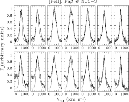
Figure 17: As in previous figure.

Figure 18: From left to right: a) nuker-law fit of the observed K-band surface brightness profile from Paper II (solid line). The dashed line is a fit with the steepest nuclear slope consistent with the data. The empty squares are the observed K band points. The filled squares are the same points after reddening correction. b) corresponding deprojected luminosity densities and c) masses enclosed within radius $r$ with $\Upsilon=1\mathrm{M}_{\odot}/\mathrm{L}_{\mathrm{K}\odot}$. The dashed area on the left represents the observed mass within 0$\farcs$25 radius and the other dashed area is the enclosed mass within 6″ required to explain the $\mathrm{H}_{2}$ rotation curve of the ring-like feature at NUC-2 with a keplerian rotation.

Figure 19: Schematic representation of the reference frames used in the determination of the keplerian rotation curve. $XY$ is the plane of the sky, $X$ is directed along the major axis of the disk, and $Z$ is directed toward the observer. $X_{disk}Y_{disk}$ is the reference frame on the disk plane such that $X_{disk}=X$ (Figure from Macchetto et al. 1997).

Table 1: Log of observations.

Band	Lines	Target Name	PA (deg)	Date (1999)	Seeing (″)
K	$\mathrm{H}_{2}$, $\mathrm{Br}\gamma$	NUCLEUS-1	32.5	May 30	0$\farcs$5
K	$\mathrm{H}_{2}$, $\mathrm{Br}\gamma$	OFF-1	32.5	May 30	0$\farcs$6
K	$\mathrm{H}_{2}$, $\mathrm{Br}\gamma$	OFF-2	32.5	May 30	0$\farcs$7
K	$\mathrm{H}_{2}$, $\mathrm{Br}\gamma$	NUCLEUS-2	135.5	Jun 3	0$\farcs$4
K	$\mathrm{H}_{2}$, $\mathrm{Br}\gamma$	OFF-2	32.5	Jun 3	0$\farcs$6
J	$[\mathrm{Fe}\,\textsc{ii}]$, $\mathrm{Pa}\beta$	NUCLEUS-1	32.5	Jun 23	0$\farcs$6
J	$[\mathrm{Fe}\,\textsc{ii}]$, $\mathrm{Pa}\beta$	NUCLEUS-1	32.5	Jul 22	0$\farcs$4
J	$[\mathrm{Fe}\,\textsc{ii}]$, $\mathrm{Pa}\beta$	NUCLEUS-2	-44.5	Jul 22	0$\farcs$4
J	$[\mathrm{Fe}\,\textsc{ii}]$, $\mathrm{Pa}\beta$	NUCLEUS-3	83.5	Jul 22	0$\farcs$5

Table 2: Fit Results.

$i$	$M_{\bullet}$	PA LoN	$V_{\mathrm{Sys}}$	$\chi_{\mathrm{Red}}^{2}$			$i$	$M_{\bullet}$	PA LoN	$V_{\mathrm{Sys}}$	$\chi_{\mathrm{Red}}^{2}$
Constant line surface brightness							Double Exponential line surface brightness
5	4357	-14.1	532	6.0			5	3832	-15.0	532	8.4
15	507	-14.3	532	6.0			15	470	-15.4	532	9.2
25	202	-14.0	532	6.1			25	177	-16.0	532	8.7
35	122	-13.6	532	6.3			35	102	-16.1	532	8.7
45	93	-13.2	532	6.7			45	72	-15.5	532	9.1
55	89	-11.8	533	7.5			55	59	-13.5	533	10.0
65	105	-10.6	533	9.3			65	55	-14.0	534	12.5
75	181	-7.8	533	13.5			75	59	-11.5	535	15.4
85	813	-2.6	533	23.3			85	68	-17.2	535	24.4

References

- Alonso-Herrero et al. (1997) Alonso-Herrero A., Rieke M.J., Rieke G.H., Ruiz M., 1997 ApJ, 482, 747
- Athanassoula & Bureau (2000) Athanassoula E., Bureau M., 2000, ApJ, 522, 699
- Bland, Taylor & Atherton (1987) Bland J., Taylor K., Atherton P.D., 1987, MNRAS, 228, 595
- Binette (1998) Binette L., 1998, MNRAS, 294, L47
- Bureau & Freeman (1999) Bureau M., Freeman K.C., 1999, AJ, 118, 126
- Bureau & Athanassoula (2000) Bureau M., Athanassoula E., 2000, ApJ, 522, 686
- Capetti et al. (2000) Capetti A., Schreier E.J., Axon D.J., Young S., Hough J.H., Clark S., Marconi A., Macchetto F.D., Packham C., 2000, ApJ, in press
- Chiaberge, Capetti & Celotti (1999) Chiaberge M., Capetti A., Celotti A., 1999, A&A, 349, 77
- De Koff et al. (1996) De Koff S. , Baum S.A., Sparks W.B., Biretta J., Golombek D., Macchetto F.D., McCarthy P., and Miley G.K., 1996, ApJS 107, 621
- Devillard (1997) Devillard, N., 1997, The Messenger 87, 19
- Di Matteo et al. (2000) Di Matteo T., Quataert E., Allen S.W., Narayan R., Fabian A.C., 2000, MNRAS311, 507
- Dufour et al. (1979) Dufour R.J., van den Bergh S., Harvel C.A., et al, 1979 AJ, 84, 284
- Eckart et al. (1990) Eckart A., Cameron M., Rothermel H., et al, 1990, ApJ, 363, 451
- Elvis et al. (1994) Elvis M., Wilkes B.J., McDowel J.C., et al, 1994, ApJS, 95, 1
- Fabian & Iwasawa (1999) Fabian A.C., Iwasawa K., 1999, MNRAS, 303, L34
- Ford et al. (1997) Ford H.C., Tsvetanov Z.I., Ferrarese L., Jaffe W., 1997, in IAU Symp. 184 ”The Central Regions of the Galaxy and Galaxies”, ed. Yoshiaki Sofue, (Dordrecht: Kluwer), p. 377
- Fukuda, Wada & Habe (1998) Fukuda H., Wada K., Habe A., 1998, MNRAS, 295, 463
- Fukuda, Habe & Wada (2000) Fukuda H., Habe A., Wada K., 2000, ApJ, 529, 109
- Hawarden et al. (1986) Hawarden T.G., Sandell G., Matthews H.E., et al, 1993, MNRAS, 260, 844
- Ho (1998) Ho L.C., 1998, in ”Observational Evidence for Black Holes in the Universe”, ed. S.K. Chakrabarti (Dordrecht: Kluwer), p. 157
- Hui et al. (1993) Hui X., Ford H.C., Ciardullo R., Jacoby G.H., 1993 ApJ, 414, 463
- Kinzer et al. (1995) Kinzer R.L., Johnson W.N., Dermer C.D., et al, 1995, ApJ, 449, 105
- Kurpiewski & Jaroszynski (2000) Kurpiewski A., Jaroszynski M., 2000, ACTA Astr. in press (astro-ph/0003418)
- Israel et al. (1990) Israel F.P., van Dishoeck E.F., Baas F., et al, 1990, A&A, 227, 342
- Israel et al. (1991) Israel F.P., van Dishoeck E.F., Baas F., et al, 1991, A&A, 245, L13
- Israel (1998) Israel F.P., 1998 A&A Rev., 8, 237
- Kormendy & Richstone (1995) Kormendy J., Richstone D., 1995, ARA&A, 33, 581
- Macchetto et al. (1997) Macchetto F.D., Marconi A., Axon D.J., Capetti A., Sparks W.B., Crane P., 1997, ApJ, 489, 579
- Macchetto (1999) Macchetto F.D., 1999, in ”Towards a New Millennium in Galaxy Morphology”, D.L. Block et al. eds. (Kluwer:Dordrecht), in press (astro-ph/9910089)
- Magorrian et al. (1998) Magorrian J., Tremaine S., Richstone D., et al, 1998, AJ, 115, 2285
- Maiolino et al. (2000) Maiolino R., Alonso-Herrero A., Anders S., et al, 2000, ApJ, 531, 219
- Malkan, Gorjian & Tam (1998) Malkan M.A., Gorjian V., Tam R., 1998, ApJS, 117, 25
- Maraston (1998) Maraston C., 1998, MNRAS, 300, 872
- Marconi et al. (1996) Marconi A., van der Werf P.P., Moorwood A.F.M., Oliva E., 1996, A&A, 315, 335
- Marconi et al. (2000) Marconi A., Schreier E.J., Koekemoer A., Capetti A., Axon D.J., Macchetto F.D., Caon N., 2000, ApJ, 528, 276
- Martel et al. (1999) Martel A.R., Baum S.A., Sparks W.B., Wyckoff E., Biretta J.A., Golombek D., Macchetto F.D., de Koff S., McCarthy P.J., Miley G.K., 1999, ApJS 122, 81
- Mathieu & Dejonghe (1999) Mathieu A., Dejonghe H., 1999, MNRAS, 303, 455
- Merrifield & Kuijken (1999) Merrifield M.R., Kuijken K., 1999, A&A, 345, L47
- Merrifield, Forbes & Terlevich (2000) Merrifield M.R., Forbes D.A., Terlevich A.I., 2000 MNRAS, 313, L29
- Mirabel et al. (1999) Mirabel I.F., Laurent O., Sanders D.B., et al, 1999 A&A, 341, 667
- Mobasher et al. (1999) Mobasher B., Guzman R., Aragon-Salamanca A., Zepf S., 1999, MNRAS, 304, 225
- Moorwood & Oliva (1988) Moorwood A.F.M., Oliva E., 1988 A&A, 203, 278
- Moorwood et al. (1999) Moorwood A.F.M., et al, 1999, The Messenger 95, 1
- Moriondo, Giovanardi & Hunt (1998) Moriondo G., Giovanardi C., Hunt L.K., 1998, A&A, 339, 409
- Narayan, Kato & Honma (1997) Narayan R. Kato S., Honma F., 1997, ApJ476, 49
- Nicholson, Bland-Hawthorn & Taylor (1992) Nicholson R.A., Bland-Hawthorn J., Taylor K., 1992, ApJ, 387, 503 (NBT92)
- Oliva & Origlia (1992) Oliva E., Origlia L. 1992, A&A, 254, 466
- Oliva (1997) Oliva E., 1997, in IAU Colloquium 159 ”Emission lines in active galaxies: new methods and techniques” ASP Conf. Ser. 113, B.M. Peterson, F.Z. Cheng A.S. Wilson eds., p. 288
- Oliva et al. (1994) Oliva E., Salvati M., Moorwood A.F.M., Marconi A., 1994, A&A, 288, 457
- Pryor & Meylan (1993) Pryor C., Meylan G., 1993, in ASP Conf. 150, ”Structure and Dynamics of Globular Clusters”, eds. S.G. Djorgovski, G. Meylan (San Francisco ASP), 357
- Quillen et al. (1992) Quillen A.C., de Zeeuw P.T., Phinney E.S., Phillips T.G., 1992 ApJ, 391, 121 (Q92)
- Quillen, Graham & Frogel (1993) Quillen A.C., Graham J.R., Frogel J.A., 1993 ApJ, 412, 550
- Regan & Mulchaey (1999) Regan M.W., Mulchaey J.S., 1999, AJ, 117, 267
- Richstone et al. (1998) Richstone D., Ajhar E.A., Bender R., et al, 1998, Nature, 395, A14
- Rydbeck et al. (1993) Rydbeck G., Wiklind T., Cameron M., et al, 1993, A&A, 270, L13
- Schreier et al. (1996) Schreier E.J., Capetti A., Macchetto F., Sparks W.B., Ford H.J., 1996 ApJ, 459, 535
- Schreier et al. (1998) Schreier E.J., Marconi A., Axon D.J., Caon N., Macchetto D., Capetti A., Hough J.H., Young S., Packham C., 1998, ApJ, 499, L143 (Paper I)
- Shloshman, Frank & Begelman (1989) Shloshman I., Frank J., Begelman M.C., 1989, Nature, 338, 45
- Soria et al. (1996) Soria R., Mould J.R., Watson A.M., et al, 1996, ApJ, 465, 79
- Tingay et al. (1998) Tingay S.J., Jauncey D.L., Reynolds J.E., et al, 1998, AJ, 115, 960
- Tonry (1991) Tonry J.L., 1991, ApJ373, L1
- Turner et al. (1997) Turner T.J., George I.M., Mushotzky R.F., Nandra K., 1997, ApJ, 475, 118
- Unger, Clegg & Stacey (2000) Unger S.J., Clegg P.E., Stacey G.J., 2000, A&A, 355, 885
- van der Marel et al. (1997) van der Marel R.P., de Zeeuw P.T., Rix H.W., Quinlan G.D., 1997, Nature385, 610
- van der Marel (1997) van der Marel R.P., 1997, in ”Galaxy Interactions at Low and High Redshift”, IAU Symposium 186, D.B. Sanders, J. Barnes eds, Kluwer Academic Publishers, p. 333
- van der Marel (1999) van der Marel R.P., 1999 AJ, 117, 744
- Wada (1994) Wada K., 1994, PASJ, 46, 165
- Wandel (1999) Wandel A., 1999, ApJ, 519, L39
- Wilkins & Axon (1992) Wilkins T.W., Axon D.J., 1992, in ASP Conf. 25, Astronomical Data Analysis Software and Systems I, eds. D.M. Worral, C. Biemesderfer, & J. Barnes (San Francisco: ASP), 427
- Wilkinson et al. (1986) Wilkinson A., Sharples R.M, Fosbury R.A.E., Wallace P.T., 1986, MNRAS218, 297
- Zhang & Pradhan (1995) Zhang H.L., Pradhan A.K., 1995, A&A, 293, 953