Time dependent cosmic–ray shock acceleration with self–consistent injection

Abstract

One of the key questions to understanding the efficiency of diffusive shock acceleration of the cosmic rays (CRs) is the injection process from thermal particles. A self–consistent injection model based on the interactions of the suprathermal particles with self–generated magneto–hydrodynamic waves has been developed recently by Malkov ([1998]). By adopting this analytic solution, a numerical treatment of the plasma–physical injection model at a strong quasi–parallel shock has been devised and incorporated into the combined gas dynamics and the CR diffusion–convection code. In order to investigate self–consistently the injection and acceleration efficiencies, we have applied this code to the CR modified shocks of both high and low Mach numbers ($M=30$ and $M=2.24$) with a Bohm type diffusion model. Both simulations have been carried out until the maximum momentum $(p_{\rm max}/m_{\rm p}c)\sim 1$ is achieved to illustrate early evolution of a Bohm type diffusion. We find the injection process is self–regulated in such a way that the injection rate reaches and stays at a nearly stable value after quick initial adjustment. For both shocks about $10^{-3}$ of the incoming thermal particles are injected into the CRs. For the weak shock, the shock has reached a steady state within our integration time and $\sim 10\%$ of the total available shock energy is transfered into the CR energy density. The strong shock has achieved a higher acceleration efficiency of $\sim 20\%$ by the end of our simulation, but has not yet reached a steady–state. With such efficiencies shocks do not become CR–dominated or smoothed completely during the early stages when the particles are only mildly relativistic. Later, as the CR pressure becomes dominated by highly relativistic particles that situation should change, but is difficult to compute, since the maximum CR momentum increases approximately linearly with time for this model. In the near future we intend to extend such shock simulations as these to include much higher CR momenta using an adaptive mesh refinement technique currently under development.

1 Introduction

The non–thermal energy distributions of cosmic ray ions or source distributions of electrons emitting synchrotron radiation in various astrophysical objects are commonly described as produced by the first order Fermi acceleration process at shocks (for reviews see Drury [1983]; Blandford & Eichler [1987]; Kirk et al. [1994]).

When particles diffuse off the moving scattering centers in a region divided by a velocity discontinuity (shock), these particles can be accelerated if their mean free paths exceed the shock thickness. The relative momentum gain for a cycle of two crossings of the shock is then proportional to the velocity difference across the shock, i.e. of first order with respect to the shock velocity (Bell [1978]). In astrophysical collisionless plasmas an electro–magnetic field must be present to change the energy of particles. Waves or irregularities in this field provide particle scattering, which leads to diffusion. Consider a shock with velocity $u_{\rm s}>0$ propagating into a plasma at rest with density $\rho$ and with a homogeneous magnetic field $B_{0}$ in the direction of the shock normal. The plasma is compressed to the density $\rho_{\rm d}$ by the shock, and flows downstream with the velocity $u_{\rm d}=u_{\rm s}(1-1/r)$, where $r=\rho_{\rm d}/\rho$ is the compression ratio. Particles with the mean downstream velocity $\langle v\rangle=u_{\rm d}$ cannot cross the shock from downstream to upstream, because $\langle v\rangle<u_{\rm s}$. In addition the shock may not be a discontinuity for a particle at this energy, because the gyro radius of the thermal particles is of the order of the shock thickness, leading to adiabatic energy change while crossing the shock. Because the plasma is also heated downstream of the shock, some supra–thermal particles in the high energy tail of the Maxwellian velocity distribution may gain energies and have velocities that allow them to re–cross the shock. In a homogeneous magnetic field, due to lack of scattering centers these particles would escape upstream without returning to the shock. Then, the acceleration mechanism would not apply. However, the population of particles that can move upstream provide a seed particle beam, which generates Alfvén waves responsible for scattering and, therefore, diffusion, which is an essential element of the first order Fermi acceleration process.

The problem of particle acceleration from thermal energies up to relativistic particle energies is highly non–linear, as first pointed out by Eichler ([1979]). First, the energy transferred from the bulk of the plasma to the sub–population of accelerated particles can change the thermodynamic properties of the plasma like the temperature and density. In addition, the accelerated particles provide their own pressure in the system, which, since it differs from the thermal pressure, modifies the velocity structure of the shock transition. Second, the waves generated by particles escaping upstream determine the transport properties of the plasma, and, therefore, regulate this wave generating escape itself. The manner in which the wave–particle interactions control the fraction of plasma particles that can escape upstream to participate in the Fermi process is commonly called injection. This is a basic aspect of the plasma of collisionless shocks and is itself highly non–linear. This injection problem is fundamentally related to the question of the efficiency of particle acceleration at shocks by the Fermi process.

Different numerical methods have been used to treat the injection problem of CR modified shocks. In Monte–Carlo simulations of non–linear particle acceleration the details of a posited scattering law provide an injection parameter, but one not determined self–consistently from the particle wave interaction (e.g. Ellison et al. [1996]; Baring et al. [1999]). In contrast to pure kinematical effects from shock velocity, particle speed and inclination angle of magnetic field and shock, the waves responsible for particle scattering depend on plasma properties like temperature and the beam strength of the wave generating particles itself. These coupled and time dependent effects are not easy to incorporate into a Monte–Carlo approach. Time dependent Monte–Carlo simulations have been presented by Knerr et al. ([1996]), but still with a prescribed scattering law, as a parameterization of injection.

In the two–fluid approach the cosmic rays are treated as a diffusive gas without following their momentum distribution. The energy transfer into CRs in these models is based on a fraction of the upstream gas particles, that are instantaneously accelerated at the shock (Dorfi [1990]), around the shock (Jones & Kang [1990]) or at velocity gradients (Zank et al. [1993]). In practical terms, because the shock is the most prominent velocity gradient in the system, these techniques are very closely related, as pointed out by Kang & Jones ([1995]). Essentially the same parameterization is also used in the numerical solution of the hydro–dynamical equations coupled to the momentum dependent cosmic–ray transport equation (e.g. Falle & Giddings [1987]; Kang & Jones [1991]; Berezhko et al. [1994]).

Kang & Jones ([1995]) used a numerical injection model with two essentially free parameters which describe boundaries in momentum at which particles can be accelerated ($p_{1}=c_{1}\cdot p_{\scriptscriptstyle\rm th}$ where $p_{\scriptscriptstyle\rm th}$ is the peak momentum of the Maxwell distribution) and from which these contribute to the cosmic–ray pressure ($p_{2}=c_{2}\cdot p_{\scriptscriptstyle\rm th}$). Still, these momentum boundaries are free parameters, which can be translated into a particle fraction of the upstream gas. However, models that incorporate more details of the plasma physics of the background plasma, and, therefore, the CRs at injection energies are really necessary to constrain the phase–space function and therefore determine these parameters. In this way we can incorporate self–consistent plasma physical models into numerical simulations of CR acceleration.

Such a plasma physical model based on non–linear interactions of particles with self–generated waves in a shocked plasma has been investigated numerically by solving the kinetic equations of ions in a magnetic field, and treating the electrons as a background fluid (Quest [1988]). These simulations show that ions can be scattered back and forth across the shock by self–generated waves, and Quest ([1988]) also points out that these scattered ions can provide a seed population of cosmic rays.

Recently, the kinetic equations of ions were solved analytically for non–linear wave–fields near strong parallel shocks by Malkov & Völk ([1995]) and Malkov ([1998]). These authors were able to constrain the fraction of phase–space of the background plasma that can be injected into the acceleration process as a result of the self–regulating interaction between wave generation and particle streaming. Here we incorporate this self–consistent analytical result in numerical solutions of the hydro–dynamical equations together with the cosmic–ray transport equation. Our simulations, therefore, provide the first time dependent solution of the problem of modified shocks that includes a self–consistent plasma physical injection model. This technique enables us to determine the level of shock modification and acceleration efficiency in an evolving shock without a free parameter for the injection process (Gieseler et al. [1999]).

We describe the plasma physical injection model in some more detail in Sect. 2 before we outline the coupled set of dynamical equations of the plasma and cosmic rays in Sect. 3, together with details of the numerical method we used to solve these equations. The results are presented in Sect. 4 and Sect. 5, consisting of the time dependent evolution of the plasma properties, showing especially the modification of the velocity profile and the momentum distributions of thermal and relativistic cosmic–ray particles. In addition we present our results in the form of a particle injection efficiency and an energy transfer efficiency at modified strong shocks.

2 Injection Model

2.1 Wave–particle interaction at parallel shocks

In supernova remnants (SNRs) the relative orientation of magnetic field and shock front can be very diverse, even in one single object. For example, if a spherically symmetric shock front expands in a region of homogeneous magnetic field, the directions of the shock normal and the magnetic field change over the shock surface from parallel to perpendicular. For nearly perpendicular shocks the acceleration process can be very fast and effective due to reflections upstream of the shock (Naito & Takahara [1995]). However, the velocity of the intersection point of shock and magnetic field in highly oblique shocks can be close to light velocity. This can suppress the injection efficiency of thermal particles, which are effectively tied to magnetic field lines. That is because the velocity distribution function of thermal protons, which we shall assume to be Maxwellian, drops sharply towards high energies. This purely kinematical effect has been investigated by Baring et al. ([1993]). Therefore, regions of SNRs where quasi–parallel shocks exist, are likely to be where the most effective injection occurs. On the other hand, effective acceleration, i.e. short acceleration time scales and hard spectra, may be realized in other parts of a SNR, where an oblique geometry of magnetic field and shock normal is found.

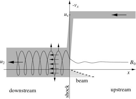
Figure 1: Cartoon of the injection model in the shock–frame phase–space. Plasma is moving towards $-x$ into the shock with velocity $-u_{\rm s}$ and gets compressed, heated and decelerated to the downstream velocity $-u_{2}$. Particles with positive velocity can stream back to upstream along the magnetic field $B_{0}$. These particles provide the beam, which generates the magnetic field waves. The magnetic field wave is shown schematically in configuration space. The wave amplitude, frequency, and damping length is shown only qualitatively.

For quasi–parallel shocks, where the shock propagates along the mean magnetic field ($x$–direction), the transport properties along the mean field direction are most important. We will assume this case, with the field $\vec{B}_{0}$ parallel to the shock normal. The spatial diffusion of particles is produced by magneto–hydrodynamic waves, which are in turn generated by particles streaming along the magnetic field, $\vec{B}_{0}$. We refer to Malkov ([1998]) for an extended analytical description of the particle–wave interaction for low–momentum particles, and we describe here only the results which are relevant for the implication of this model in our simulations of the time dependent acceleration at modified shocks. When particles are streaming along the magnetic field in the upstream direction, waves are generated due to the ion cyclotron instability. The resulting upstream magnetic field, which corresponds to a circularly polarized wave, can be written as

$$\vec{B}=B_{0}\vec{e}_{x}+B_{\scriptscriptstyle\bot}(\vec{e}_{y}\cos k_{0}x-\vec{e}_{z}\sin k_{0}x).$$ (1)

The amplitude $B_{\scriptscriptstyle\bot}$ will be amplified downstream of the shocks by a factor $r=\rho_{\rm d}/\rho$. The downstream field can be described by a parameter $\epsilon$, for which, following Malkov, we assume $\epsilon:=B_{0}/B_{\scriptscriptstyle\bot}\ll 1$, in the case of strong shocks. Note that the perpendicular component of the magnetic field leads effectively to an alternating field downstream of the shock for particles moving along the shock normal (see Fig. 1).

2.2 Thermal leakage model

The particles with a large enough gyro radius

$$r_{{\rm g}\scriptscriptstyle\bot}=p\,c\,\sin\alpha/(eB_{\scriptscriptstyle\bot})>1/k_{0}$$ (2)

can have an effective velocity with respect to the wave frame, i.e. the downstream plasma would be transparent. Some of these particles that are in the appropriate part of the phase space (depending on the shock speed) would be able to cross the shock from downstream to upstream. For the protons of the plasma, the resonance condition for the cyclotron generation of the Alfvén waves gives $k_{0}\langle v\rangle\approx\omega_{0}=\omega_{\scriptscriptstyle\bot}B_{0}/B_{\scriptscriptstyle\bot}$, where the cyclotron frequency of protons is given by $\omega_{\scriptscriptstyle\bot}=eB_{\scriptscriptstyle\bot}/(m_{\rm p}c)$, and $\langle v\rangle$ is the mean downstream thermal velocity of the protons. We now have for the thermal protons $k_{0}r_{{\rm g}\scriptscriptstyle\bot}\approx\epsilon\ll 1$. This means that most of the downstream thermal protons would be confined by the wave, and only particles with higher velocity in the tail of the Maxwellian distribution are able to leak through the shock. Ions with mass–to–charge ratio higher than protons have a proportionally larger gyro radius, so that the injection efficiency of protons would yield a lower limit for the less magnetized ions. On the other hand, for thermal electrons a plasma with such proton generated waves would have a reduced transparency due to the smaller gyro radius of the electrons. However, reflection of electrons (and protons) off the shock could become efficient with increasing wave amplitude and possibly aid in their injection (e.g. Levinson [1996]; McClements et al. [1997]). In the following we will focus on the protons, which carry most of the energy and momentum of the plasma.

2.3 Transparency function

Figure 2: Transparency function Eq. (3) vs. the normalized particle velocity $\tilde{v}=vk_{0}/\omega_{\scriptscriptstyle\bot}$ for $\epsilon=0.35$ (solid line). Shown as a dashed line is the transparency function given in Fig. 2 of Malkov & Völk (1998).

To find the part of the thermal distribution for which the magnetized plasma is transparent, and, which, therefore, forms the “injection pool”, Malkov ([1998]) solves analytically the equations of motion for protons in self–generated waves. He finds a transparency function $\tau_{\rm\scriptscriptstyle esc}$, which expresses the fraction of particles that are able to leak through the magnetic waves, divided by the part of the phase space for which particles would be able to cross from downstream to upstream when no waves are present. For the adiabatic wave particle interaction the transparency function is given by Malkov ([1998]) Eq. (33), with $\tau_{\rm\scriptscriptstyle esc}=2\,\nu_{\rm\scriptscriptstyle esc}/(1-u_{2}/v)$, where $v$ is the particle velocity $v$ and $u_{2}=u_{\rm s}/r$ is the velocity of the shock in the downstream plasma frame. Here $\nu_{\rm\scriptscriptstyle esc}$ is the fraction of the particles streaming back from downstream to upstream. This quantity is divided by the fraction of particles that would be able to escape upstream in the absence of waves. In order not to further increase the complexity of our numerical simulation, we use here the following approximation of the representation given in Malkov ([1998]):

$$\tau_{\rm\scriptscriptstyle esc}(v,u_{2}) = H\left[\tilde{v}-(1+\epsilon)\right]\left(1-\frac{u_{2}}{v}\right)^{-1}\,\left(1-\frac{1}{\tilde{v}}\right)$$ (3)

$$\cdot\exp\left\{-\left[\tilde{v}-(1+\epsilon)\right]^{-2}\right\}\,,$$

where the particle velocity is normalized to $\tilde{v}=vk_{0}/\omega_{\scriptscriptstyle\bot}$ and $H$ is the Heaviside step function. We argued above that $\omega_{\scriptscriptstyle\bot}/k_{0}\simeq u_{2}/\epsilon$ (see Malkov [1998], Eq. 42). The transparency function now solely depends on the shock velocity in the downstream flow frame, $u_{2}$, the particle velocity, $v$, and the relative amplitude of the wave, $\epsilon$.

The calculation of the transparency function and the wave–amplitude $\epsilon$ uses the ergodicity of the downstream phase–space for the randomized motion of particles in the high–amplitude wave field. The upstream wave field is generated by a beam of leaking particles whose energy density is calculated from the corresponding area of the downstream phase–space. From the energy density of this beam the upstream magnetic–field wave amplitude is determined self–consistently (Malkov [1998]). Because of this feedback Malkov was able to constrain the quantity $\epsilon$ as $0.3\la\epsilon\la 0.4$, leaving essentially no free parameter.

Figure 3: Transparency function Eq. (3) vs. the normalized particle velocity $\tilde{v}=v/u_{2}$ for different values of $\epsilon$. We used the relation $\omega_{\scriptscriptstyle\bot}/k_{0}\simeq u_{2}/\epsilon$ (see text).

Comparison with hybrid plasma simulations suggests $0.25\la\epsilon\la 0.35$ (Malkov & Völk [1998]), consistent with their analytical results. This constraint on the wave–amplitude $B_{\scriptscriptstyle\bot}/B_{0}=1/\epsilon$ defines the level to which the particle–wave interaction adjusts. With the estimation of this amplitude there is no free parameter describing the level of the beam strength for the injection, and, therefore, the injection efficiency. The advantage of our approach presented here is that quantities like the plasma velocity and particle momentum distribution are calculated self–consistently by solving simultaneously the hydro–dynamical equations together with the cosmic–ray transport equation (see Sect. 3.1).

The function (3) is plotted in Fig. 2 for $\epsilon=0.35$ vs. the particle velocity normalized to $\tilde{v}=vk_{0}/\omega_{\scriptscriptstyle\bot}$. In Fig. 2 we have also reproduced this function as given in Fig. 2 of Malkov & Völk ([1998]) to allow a direct comparison. The strong velocity dependence and also the asymptotic behavior is modeled reasonably well by the representation Eq. (3). In the normalization of Fig. 2, the dependence on $\epsilon$ is very weak, and, therefore, not shown. To illustrate the dependence of the transparency function on small variations of the field amplitude, it is better to choose a different normalization. Therefore, the transparency function Eq. (3) is shown in Fig. 3 vs. the velocity normalized to $\tilde{v}=v/u_{2}$ for the maximal allowed range in $\epsilon$, as described above.

3 Model

3.1 Dynamical equations

The standard hydro–dynamical equations of mass, momentum and energy conservation for a gas with velocity $u(x,t)$, and density $\rho(x,t)$, corrected for CR pressure effects are given by

$$\frac{{\rm d}\rho}{{\rm d}t} = -\rho\frac{\partial u}{\partial x}\,,$$ (4)

$$\rho\frac{{\rm d}u}{{\rm d}t} = -\frac{\partial}{\partial x}(P_{\rm g}+P_{\rm c})\,,$$ (5)

$$\rho\frac{{\rm d}e_{\rm g}}{{\rm d}t} = -\frac{\partial}{\partial x}\left[u(P_{\rm g}+P_{\rm c})\right]+P_{\rm c}\frac{\partial u}{\partial x}-S(x,t)\,,$$ (6)

where $P_{\rm g}$ and $P_{\rm c}$ are the gas and the CR pressure, respectively, and $e_{\rm g}={P_{\rm g}}/{\rho}(\gamma_{\rm g}-1)+u^{2}/2$ is the total energy density of the gas per unit mass. Here ${{\rm d}}/{{\rm d}t}\equiv{\partial}/{\partial t}+u{\partial}/{\partial x}\,$ is the total Lagrangian time derivative. We assume $\gamma_{\rm g}=5/3$ for the thermal gas adiabatic index throughout this work. The injection energy loss term $S(x,t)$ accounts for the energy transferred to high energy particles and will be discussed later. Equations (4)–(6) are solved using a Total Variation Diminishing (TVD) code based on the scheme of Harten ([1983]).

We assume that the shock Mach number $M=u_{\rm s}/c_{\rm s}$ (with $c_{\rm s}=(\gamma P/\rho)^{1/2}$ the upstream sound speed) exceeds the Alfvén Mach number $M_{\rm A}=u_{\rm s}/c_{\scriptscriptstyle\rm A}\ll M$ (with $c_{\scriptscriptstyle\rm A}=B/(4\pi\rho)^{1/2}$ the upstream Alfvén speed). Then the diffusion–convection equation, which describes the time evolution of the phase–space density $f(p,x,t)$ of the high energy CRs (e.g. Skilling [1975]), takes the form:

$$\frac{{\rm d}f}{{\rm d}t} = \frac{1}{3}\frac{\partial u}{\partial x}p\,\frac{\partial f}{\partial p}+\frac{\partial}{\partial x}\left(\kappa(x,p)\frac{\partial}{\partial x}f\right)\,.$$ (7)

The diffusion coefficient $\kappa(p,x)$ is assumed to be a scalar. Transforming to the variables $y:=\ln(p)$ and $g(y,x,t):=p^{4}f(p,x,t)$ (cf. Falle & Giddings [1987]; Kang & Jones [1991]), Eq. (7) can be written as

$$\frac{{\rm d}g}{{\rm d}t} = \frac{1}{3}\frac{\partial u}{\partial x}\left(\frac{\partial g}{\partial y}-4g\right)+\frac{\partial}{\partial x}\left(\kappa(y,x)\frac{\partial}{\partial x}g\right)\,.$$ (8)

This equation is solved using an implicit Crank–Nicholson scheme, which is second order in space and time (see e.g. Falle & Giddings [1987]).

The high energy particles provide an additional pressure to the system that has to be included in the set of hydro–dynamical equations (with $p$ normalized to the proton momentum $p/m_{\rm p}c\to p$):

$$P_{\rm c} = \frac{4}{3}\pi m_{\rm\scriptscriptstyle p}c^{2}\int\limits_{0}^{\infty}(f-f_{\scriptscriptstyle\rm M})\,p^{4}\frac{{\rm d}p}{\sqrt{p^{2}+1}}\,.$$ (9)

This definition of the CR pressure $P_{\rm c}$ includes the difference of the phase–space density from the Maxwellian distribution $f_{\scriptscriptstyle\rm M}$ and defines the sub–population which we identify as CRs. The CR energy density is defined as

$$E_{\rm c} = 4\pi m_{\rm\scriptscriptstyle p}c^{2}\int\limits_{0}^{\infty}(f-f_{\scriptscriptstyle\rm M})\,p^{2}(\sqrt{p^{2}+1}-1)\,{\rm d}p\,.$$ (10)

3.2 Injection scheme

We do not include an additional injection term in Eq. (8), because in our model injection is described self–consistently from the thermal distribution. Therefore, the lower boundary of the momentum distribution of the CR population must match the upper boundary of the momentum distribution of the gas. The distinction between these populations is, of course, only technical, and defined by the validity of the relevant dynamical equations. We use a Maxwell distribution according to the actual density and temperature of the plasma. Instead of a fixed momentum boundary we use here the transparency function $\tau_{\rm\scriptscriptstyle esc}$ to define where the lower boundary of the CR momentum distribution matches the momentum distribution of the bulk plasma. The injection into the high energy part of the phase–space distribution (i.e. the CRs) is then directly provided by the bulk of the plasma.

The initial Maxwellian phase–space density $f_{\scriptscriptstyle\rm M}(p,x,t)$ is given by:

$$g_{\scriptscriptstyle\rm M}(p,x,t) = p^{4}f_{\scriptscriptstyle\rm M}(p,x,t)$$ (11)

$$= \frac{n(x,t)p^{4}}{(2\pi m_{\rm p}\,k_{\rm\scriptscriptstyle B}T)^{3/2}}\exp\left(\frac{-p^{2}}{2m_{\rm p}\,k_{\rm\scriptscriptstyle B}T}\right),$$

where $n(x,t)=\rho/m_{\rm p}$ is the particle number density, and the temperature is defined by the local gas pressure $P_{\rm g}$ and density $\rho$ according to $T=\mu m_{\rm p}P_{\rm g}/\rho k_{\rm\scriptscriptstyle B}$. Here $\mu$ is the mean molecular weight which is assumed to be one, and $k_{\rm\scriptscriptstyle B}$ is the Boltzmann constant. The details of how the momentum distribution is calculated in a time step from $t-\Delta t$ to $t$ are as follows. First we define the CR part of the momentum distribution by $g_{\scriptscriptstyle\rm CR}(t-\Delta t)=g(t-\Delta t)-g_{\scriptscriptstyle\rm M}(t-\Delta t)$. Now the CR diffusion–convection equation (Eq. 8) is solved for the entire momentum space, including the thermal Maxwell distribution, to find the updated distribution function $\tilde{g}(p,x,t)$. For momenta below the critical momentum of $\tau_{\rm\scriptscriptstyle esc}(p_{\rm crit})\equiv 0$ any particle acceleration must be suppressed, and therefore the result of Eq. (8) is rejected by restoring the Maxwellian distribution given in Eq. (11). For momenta above the critical momentum and upstream of the shock, we use the transparency function as a filter for $\tilde{g}(p,x,t)$ as described below, since $\tau_{\rm\scriptscriptstyle esc}(p,t)$ corresponds to the fraction of the phase–space density at a given momentum that can cross the shock from downstream to upstream. The final distribution at time $t$ is then given by $g(p,x,t)$ in the following way:

$$\tilde{g}_{\scriptscriptstyle\rm CR}(p,x,t) = \tilde{g}(p,x,t)-g_{\scriptscriptstyle\rm M}(p,x,t)\,,$$ (12)

$$g_{\scriptscriptstyle\rm CR}(p,x,t) = g_{\scriptscriptstyle\rm CR}(p,x,t-\Delta t)+\tau_{\rm esc}(p,t)$$ (13)

$$\cdot\left[\tilde{g}_{\scriptscriptstyle\rm CR}(p,x,t)-g_{\scriptscriptstyle\rm CR}(p,x,t-\Delta t)\right]\,,$$

$$g(p,x,t) = g_{\scriptscriptstyle\rm CR}(p,x,t)+g_{\scriptscriptstyle\rm M}(p,x,t)\,.$$ (14)

So effectively at the lower momentum limit where $\tau_{\rm\scriptscriptstyle esc}(p)\equiv 0$ the Eq. (8) has no effect at all, while at the higher momentum limit where $\tau_{\rm\scriptscriptstyle esc}(p)\equiv 1$ the result of Eq. (8) is used without further modification. Only in the intermediate momentum regime where $0<\tau_{\rm\scriptscriptstyle esc}(p)<1$, the transparency function represents the injection process (i.e. thermal leakage). Thus the transparency function defines self–consistently the momentum boundary above which the particle acceleration mechanism can work, and also defines the transition region between thermal plasma and accelerated particles.

The particle injection rate into the CR population can be estimated from the adiabatic change of the momentum due to the velocity gradient of the flow:

$$Q(p,x,t) = 4\pi\,p^{2}f(p,x,t)\,\left(\frac{\partial p^{\prime}}{\partial t}\right)_{p}$$ (15)

$$= -\frac{4\pi}{3}p^{3}f(p,x,t)\frac{\partial u}{\partial x}\,.$$

Then the energy loss rate of the gas can be written as

$$S(x,t) = \frac{1}{2}m_{\rm p}c^{2}\int\limits_{0}^{\infty}\frac{\partial\tau_{\rm\scriptscriptstyle esc}(p,t)}{\partial p}p^{2}Q(p,x,t)\,{\rm d}p\,,$$

$$= -\frac{2}{3}\pi\,m_{\rm p}c^{2}\,\frac{\partial u}{\partial x}\int\limits_{0}^{\infty}\frac{\partial\tau_{\rm\scriptscriptstyle esc}(p,t)}{\partial p}p^{5}f(p,x,t)\,{\rm d}p\,.$$

Note here the condition ${\partial\tau_{\rm\scriptscriptstyle esc}(p,t)}/{\partial p}\not=0$ in fact defines the “injection pool” where the thermal leakage takes place. Due to the steep dependence of both the Maxwell distribution and the transparency function on the particle momentum, the momentum range of the injection pool is well restricted. Either below or above this momentum range $\tau_{\rm\scriptscriptstyle esc}(p)=$ constant, so ${\partial\tau_{\rm\scriptscriptstyle esc}(p,t)}/{\partial p}=0$. If the transparency function is given by a step function $\tau_{\rm\scriptscriptstyle esc}(p)=H(p-p_{\scriptscriptstyle\rm inj})$, it becomes the injection scheme adopted by Kang & Jones ([1995], [1997]) in which the injection takes place at a single injection momentum rather than an extended momentum range.

The transparency function $\tau_{\rm\scriptscriptstyle esc}$ given by Eq. (3) depends on the downstream plasma velocity, which is averaged over the diffusion length of the particles with momentum at the injection threshold. This dependence is also important for the injection efficiency, and leads to a regulation mechanism similar to the above beam wave interaction. If the initial injection is so strong that a significant amount of energy is transferred from the gas to high energy particles, the downstream plasma cools, and, in addition, the downstream bulk velocity decreases in the shock frame due to the shock modification of the cosmic–ray population. Because the injection pool is in the high energy tail of the Maxwellian distribution of the gas, the cooling decreases significantly the injection rate. However, the deceleration, in turn, allows for a modest increase of the phase–space of particles that can be injected. This is expressed by the $u_{2}$ dependence of Eq. (3). This velocity dependence balances partly the reduction of injection due to the cooling of the plasma. Remarkably, these two effects lead to a very weak dependence of the injection efficiency on $\epsilon$ in the vicinity of $\epsilon\approx 0.35$.

3.3 Diffusion model

Since the injection process is included self–consistently, the diffusion coefficient is the only remaining free parameter in our model. We assume the particle diffusion is based on the scattering off the self–generated waves which have a field component perpendicular to the plasma flow. The compression of the plasma leads to an amplification of these waves, which is described by scaling the diffusion coefficient as $\kappa\propto 1/\rho$. In our one dimensional model we have to describe diffusion along the mean magnetic field. The lower limit for the diffusion coefficient is the Bohm diffusion coefficient $\kappa_{\rm\scriptscriptstyle B}(p)=(3\cdot 10^{22}~{}{{\rm cm}^{2}}/{\rm s}/B_{\mu{\rm G}})~{}{p^{2}}/{(1+p^{2})^{1/2}}\,,$ where $B_{\mu{\rm G}}$ is the magnetic field strength in units of micro–gauss. For the present calculations we assume the diffusion coefficient is simply related to Bohm diffusion as

$$\kappa(p)=\zeta\,~{}\kappa_{\rm\scriptscriptstyle B}\,\rho_{0}/\rho(x)\,.$$ (17)

We have introduced the factor $\zeta$ to account for the higher diffusion in the direction of the mean magnetic field, because this direction is parallel to the shock normal, and, therefore, relevant for the acceleration process at quasi–parallel shocks. Although the time scale for the cosmic–ray acceleration does depend on the diffusion coefficient, the basic self regulation process for the injection problem which we investigate here is not dependent on the choice of $\zeta$. Therefore, since our study intends to focus on the general time dependent behavior of this injection model, we do not include a completely self–consistent scattering model, where the diffusion coefficient is coupled to the spectrum of the Alfvén waves.

3.4 Initial and boundary conditions

We assume there is no pre–existing CR population, so the initial particle distribution is purely Maxwellian with the local plasma temperature and density. We use open boundary conditions for the description of the thermal plasma in our simulations. In momentum space, the lower boundary is provided by the Maxwell distribution as discussed above. At the highest momentum and also at the upstream boundary in configuration–space we use a ‘free escape’ boundary. Downstream we use a ‘no diffusive flux’ boundary, where the cosmic–ray density is always kept constant across the boundary. However, the grid size was chosen so large in the simulations we present here, that the cosmic–ray pressure is at all times essentially zero at both boundaries.

4 Results for strong shocks

First we consider a strong shock with an initial Mach number of $M=30$. Unlike an ordinary hydrodynamic simulation, the simulation of the CR shock acceleration requires specification of three physical parameters, $u_{0}/c$, $\rho_{0}/m_{\rm p}$, and the shock Mach number in addition to the diffusion coefficient. We adopted the following nominal physical scales for physical parameters: $u_{0}=5000\,{\rm km\,s}^{-1}$, $\rho_{0}/m_{\rm p}=0.03\,{\rm cm}^{-3}$, $t_{0}=4.0\cdot 10^{4}$ s, $x_{0}=2.0\cdot 10^{13}$ cm, $P_{\rm g0}=\rho_{0}u_{0}^{2}=1.25\cdot 10^{-8}\,{\rm erg\,cm}^{-3}$. We use $\zeta=100$ for the simulations presented here, and a magnetic field of $B=3\mu$G. The initial conditions are specified as follows: $\rho_{\rm up}=\rho_{0}$, $u_{\rm up}=-u_{0}$, and $P_{\rm g,up}=6.667\cdot 10^{-4}P_{\rm g0}$ in the upstream region, while $\rho_{\rm d}=3.987\rho_{0}$, $u_{2}=-0.25u_{0}$, $P_{\rm g,d}=0.75P_{\rm g0}$ downstream. These values reflect the shock jump conditions in the rest–frame of the shock.

We define the diffusion length and time at a given momentum as $l_{\rm d}(p)=\kappa(p)/u_{0}$ and $t_{\rm d}(p)=\kappa(p)/u_{0}^{2}$. For a proper convergence, the spatial grid size should be smaller than the diffusion length of the injection pool particles ($l_{\rm d}/x_{0}\sim 0.04$ in upstream for $p_{\scriptscriptstyle\rm inj}\sim 0.02$). On the other hand, the spatial region of the calculation in upstream and downstream should be larger than the diffusion length–scale of the particles with the highest energies reached at the end of our simulation period ($l_{\rm d}/x_{0}\sim 230$ for $p_{\rm max}\sim 2.5$). So we used 51200 uniform grid zones for $x/x_{0}=[-250,250]$, with the shock initially at $x=0$ and the grid size $\Delta x/x_{0}=0.01=0.25\cdot l_{\rm d}(p_{\scriptscriptstyle\rm inj})/x_{0}$. We use 128 uniform grid zones in $\log(p)$ for $\log(p)=[-3.0,0.477]$. We integrate the solutions until $t=240t_{0}$ which corresponds to $t_{\rm d}$ for $p_{\rm max}\sim 2.5$, so the CR particles became only mildly relativistic by the end of our simulations.

Figure 4: Gas density $\rho/\rho_{0}$, pressure $P_{\rm g}/P_{\rm g0}$, velocity $u/u_{0}$, and cosmic–ray pressure $P_{\rm c}/P_{\rm g0}$, at times $t=0$ (dotted), $t=120\,t_{0}$ (dashed) and $t=240\,t_{0}$ (solid line). The shock Mach number is $M=30.0$, $\epsilon=0.35$ and $\zeta=100$. The initial upstream gas pressure is $P=6.667\cdot 10^{-4}P_{\rm g0}$.

4.1 Dynamical evolution

Figure 4 shows the normalized gas density $\rho(x)$, gas pressure $P_{\rm g}(x)$, plasma velocity $u(x)$ and the cosmic–ray pressure $P_{\rm c}(x)$ over the spatial length $x$, for different times. This shows clearly the basic features of the shock modification by a diffusive component; that is, the adiabatic precursor compression and the sub–shock. The CR pressure $P_{\rm c}$ is responsible for the deceleration and compression of the plasma flow in the precursor region upstream of the sub–shock, which still remains strong. As a result, the gas is compressed to higher density downstream of the sub–shock.

The cosmic–ray pressure immediately downstream of the sub–shock has not reached a steady state yet. The reason is that for a the non–thermal particles with a momentum distribution $f\propto p^{-s}$ with $s\leq 4$, the energy density is an increasing function of $p_{\rm max}$. This applies even if the injection is shut down completely, like for an $\delta$–function type injection in time, as shown by Drury ([1983]). We expect that $P_{\rm c}$ will continue to increase after our integration time $t=240t_{0}$, which leads to a significant modification of the shock structure and to the steepening of the power–law distribution of suprathermal particles. The simulations of such non–linear evolution, however, require much greater spatial region and grid zones and also longer integration time than what we could afford in our simulations.

In real astrophysical shocks, the energy density is limited by radiation losses in the case of electrons or more generally by particle escape due to the finite extent of the acceleration region. For the maximum energy of particles ($p_{\rm max}\sim 2.5$) achieved by $t=240\,t_{0}$ in this simulation, neither effect is important, and, therefore, not included.

4.2 Energy distribution

Figure 5: Phase–space density $g=p^{4}f$ vs. proton momentum immediately downstream of the sub–shock. Also shown is the transparency function $\tau_{\rm\scriptscriptstyle esc}$. Both functions are presented for $t=0$ (dotted), $t=10\,t_{0}$ (dot–dashed), $t=120\,t_{0}$ (dashed), and $t=240\,t_{0}$ (solid line). For the parameters used see Fig. 4 and corresponding text.

The phase–space distribution $g(p,x,t)\equiv p^{4}\,f(p,x,t)$ immediately (three zones) behind the sub–shock is shown in Fig. 5 for three different times. Initially this distribution is given by a Maxwell distribution, as shown by the dotted line. At the thermal part of the distribution the cooling of the postshock gas due to the energy flux into the CR particles is responsible for the shift of the Maxwellian distribution towards lower energies. We have also plotted the transparency function $\tau_{\rm\scriptscriptstyle esc}$ at the same simulation times. According to Eq. (3.2) the injection rate into the non–thermal distribution depends on overlap of ${\partial\tau_{\rm\scriptscriptstyle esc}}/{\partial p}$ and $g(p)$ that determines the injection pool. One can see that initially the injection rate is high and so the postshock gas cools quickly, resulting in narrowing down of the injection pool. This causes the injection rate to decrease. But then the transparency function also shifts toward lower momenta, because the downstream plasma velocity $u_{2}$ decreases as the postshock gas cools. The combination of the shift of $\tau_{\rm\scriptscriptstyle esc}$ toward lower momenta and the decrease of the particles in the Maxwellian tail due to the gas cooling leads to the self–regulation of the injection rate at a quite stable value. According to the plot of $g(p)$ at $t=120\,t_{0}$ and $t=240\,t_{0}$, the Maxwell distribution turns into a power–law at an almost constant “effective injection momentum” which determines the magnitude of the CR distribution function $g(p)$ at a stable value (about $1/200$ of the thermal peak). The value of this constant effective injection momentum can be translated into the parameter $c_{1}=p_{\scriptscriptstyle\rm inj}/p_{\scriptscriptstyle\rm th}\sim 2.3$ (where $p_{\scriptscriptstyle\rm th}=2\sqrt{m_{\rm p}k_{\rm\scriptscriptstyle B}T}$) defined by Kang & Jones ([1995]). But this is somewhat larger than what they used ($c_{1}=1.9-1.95$).

Figure 6: Omni–directional flux vs. proton kinetic energy, for $t=0$ (dotted), $t=10\,t_{0}$ (dot–dashed), $t=120\,t_{0}$ (dashed), and $t=240\,t_{0}$ (solid line). These distributions are identical to those shown in Fig. 5. For the parameters used see Fig. 4 and corresponding text.

The narrow injection pool also leads to a rather sharp transition from the Maxwell distribution to the non–thermal part starting shortly above the effective injection momentum (see Fig. 5). The canonical result in the test particle limit, $g(p)=p^{4}\,f(p)=p^{4}\,p^{-s}=$ constant, for a strong shock with $s=3r/(r-1)=4$ is reproduced very well in our simulations. The same energy spectrum is shown in Fig. 6 in the form of the omni–directional flux $F(E){\rm d}E\propto v\,p^{2}f(p){\rm d}p$ vs. proton kinetic energy downstream of the shock normalized to $t=0$. At energies above the injection pool we expect, for the strong shock ($r\simeq 4$) simulated here, the result $F(E)\propto E^{-\sigma}$, with $\sigma=\{(r+2)/(r-1)\}/2=1$, which is reproduced with high accuracy.

In using the standard cosmic–ray transport equation, we have, of course, made use of the diffusion approximation, which may introduce an error especially for $v\simeq u_{2}$. Using an eigenfunction method, Kirk & Schneider ([1989]) have explicitly calculated the angular distribution of accelerated particles and accounted for effects of a strong anisotropy especially at low particle velocities. They were able to calculate the injection efficiency without recourse to the diffusion approximation, and found always lower efficiencies compared to those in the diffusion approximation. Using the initial thermal distribution, we have estimated an effective injection momentum from the peak of the distribution function, $g_{\scriptscriptstyle\rm M}(p)\tau_{\rm\scriptscriptstyle esc}(p)$. For the shock parameters considered here and for $\epsilon=0.35$ we get an effective initial injection velocity of about $6700\,{\rm km\,s}^{-1}$ (in the shock frame). For this injection velocity, $r=4$ and $u_{0}=5000\,{\rm km\,s}^{-1}$, they estimate a reduction effect of $\approx 8\%$, leaving the diffusion approximation as quite reasonable even in this regime.

4.3 Injection and acceleration efficiencies

To describe the injection efficiency often a parameter $\xi$ is used for the fraction of the in–flowing plasma particles that are instantaneously accelerated to a fixed injection momentum $p_{\scriptscriptstyle\rm inj}$ (e.g. Falle & Giddings [1987]; Dorfi [1990]; Jones & Kang [1990]; Zank et al. [1993]; Berezhko et al. [1994]). The injection energy flux $I$ transferred to CRs is then given by

$$I=\xi\,\frac{\rho_{1}u_{1}}{m}\,\frac{p_{\scriptscriptstyle\rm inj}^{2}}{2m}\,,$$ (18)

where $u_{1}$ is the upstream plasma velocity in the shock frame, and $\rho_{1}$ is the upstream density. From the fact that the injected energy flux $I$ must be equal to the spatial integral of the injection energy loss term $S(x)$, that is, $I=\int S(x)\,{\rm d}x$ and by assuming momentarily a step function for the transparency $\tau_{\rm\scriptscriptstyle esc}(p)=H(p-p_{\scriptscriptstyle\rm inj})$, we get:

$$\xi(t)=-\frac{4\pi}{3}\,\int\frac{\partial u}{\partial x}\frac{p_{\scriptscriptstyle\rm inj}^{3}f(p_{\scriptscriptstyle\rm inj})}{n_{1}\,u_{1}}\,{\rm d}x\,,$$ (19)

where $n_{1}=\rho_{1}/m$ is the upstream number density. This is equivalent to the injection parameter used by Kang & Jones ([1995]). The so–defined injection parameter $\xi$ is, however, not an exact measure of the number of particles contributing to the population of cosmic rays, because the acceleration process cannot be described by shifting particles instantaneous from thermal energies to an injection momentum $p_{\scriptscriptstyle\rm inj}$. Furthermore, $\xi$ depends strongly on the chosen injection momentum $p_{\scriptscriptstyle\rm inj}$, which is not a fixed single parameter in our numerical simulation.

A method to measure the injection efficiency without specifying the injection momentum, is to compare the number of particles in the CR part to the number of particles swept through the shock. According to our definition of the CR population we can write for the CR number density

$$n_{\scriptscriptstyle\rm CR}(x,t) = \int f_{\scriptscriptstyle\rm CR}(p,x,t){\rm d}^{3}p$$ (20)

$$\equiv \int\left(f(p,x,t)-f_{\scriptscriptstyle\rm M}(p,x,t)\right){\rm d}^{3}p\,.$$

The fraction of particles that has been swept through the shock after the time $t$, and then injected into the cosmic–ray distribution is then given by

$$\xi^{*}(t)=\frac{\int n_{\scriptscriptstyle\rm CR}(x,t){\rm d}x}{n_{1}u_{1}\,t}\,.$$ (21)

The time development of this injection efficiency is plotted in Fig. 7 for three values of the inverse wave amplitude $\epsilon$. Recall that Malkov ([1998]) found $0.3\la\epsilon\la 0.4$.

Figure 7: Energy efficiency $\eta(t)$ and the fraction of cosmic–ray particles $\xi^{*}(t)$ for three values of the inverse wave–amplitude $\epsilon$ at a strong, $M=30$, shock. For the parameters used see Fig. 4 and corresponding text.

In the very beginning of the simulation the injection does depend strongly on the wave–amplitude, because of the very steep dependence of the Maxwell distribution at the injection energies. However, as described above, a strong initial injection leads to a temperature decrease of the plasma, and to a shift of the Maxwell distribution, which balances this effect. Therefore at later times the fraction of injected particles, $\xi^{*}$, does not depend strongly on the initial wave–amplitude. At time $t/t_{0}=250$ (or $t=1.0\cdot 10^{7}$s) we get a fraction of injected particles of $\xi^{*}=(1.5\pm 0.4)\cdot 10^{-3}$ for the interval $\epsilon=0.35\pm 0.5$.

To measure the efficiency of the particle acceleration at a shock front, we compare the energy flux in cosmic rays to the total energy which is available from the downstream plasma flow. This energy consists of the sum of kinetic energy and the gas enthalpy. The fraction of this initial energy flux, which is transferred to CRs is given by

$$\eta(t) = \frac{\frac{\gamma_{\scriptscriptstyle\rm c}(t)}{\gamma_{\scriptscriptstyle\rm c}(t)-1}u_{\rm d}(t)P_{\rm c}(t)}{\frac{1}{2}\rho_{\rm d}u_{\rm d}^{3}+\frac{\gamma_{\scriptscriptstyle\rm g}}{\gamma_{\scriptscriptstyle\rm g}-1}u_{\rm d}P_{\rm g,d}}\,,$$ (22)

where $u_{\rm d}=u_{\rm s}(1-1/r)$ is the initial downstream plasma velocity in the upstream rest frame. The definition of the efficiency $\eta(t)$ is similar to the definition from Völk et al. ([1984]). However, Eq. (22) compares the energy flux in CRs not only to the kinetic energy flux of the gas, but also includes the gas enthalpy flux. We measure the CR pressure immediately downstream of the sub–shock, where it will first reach the constant downstream value, in case a steady state does exist (see below). The time dependent values are averaged over the interval $x/x_{0}=[-0.5u_{2}t,\dots,0]$ in the shock frame to avoid influence of small scale modifications of the cosmic–ray pressure and plasma velocity on the injection efficiency. When the quantities $u_{2}$, $P_{\rm c}$ and $\gamma_{\rm c}$ have reached steady–state distributions downstream of the sub–shock, $\eta(t)$ is also no longer time dependent.

The evolution of the energy efficiency, $\eta(t)$, is plotted in Fig. 7 for three different magnetic–field wave amplitudes. See Fig. 4 and the description in Sect. 4 for the corresponding parameters. The case $\epsilon=0.4$ corresponds to the highest injection efficiency and therefore leads to the highest cosmic–ray pressure. To assure a vanishing value of the cosmic–ray pressure at the spatial grid boundaries at all times, the calculation for $\epsilon=0.4$ was done on a somewhat larger grid with 60416 uniform zones for $x/x_{0}=[-300,300]$. For the value $\epsilon=0.35$, which was calculated by Malkov ([1998]), we see that about 20% of the available energy in this shock is transferred into the cosmic–ray population. The acceleration efficiency has, however, not reached a real steady state value, but is increasing with $\eta(t)\propto t^{\alpha}$ with $\alpha\approx 0.1$. The acceleration efficiency achieved by this time is given by $\eta=(18\pm 5)\%$ for $\epsilon=0.35\pm 0.5$. Thus a substantial amount of the initial energy flux at a shock front can be transferred to a high energy part of the distribution, during the relatively short time we have simulated here.

5 Results for weak shocks

When the initial compression ratio decreases for a weak shock, the injection process is influenced in several ways by the change in the plasma and magnetic field properties. To investigate the effects of a lower compression ratio and lower Mach number on the injection process we will consider an example with $r=2.5$ and $M=2.24$. At such a shock, the phase space for which the downstream particles can re–cross the shock to upstream is decreased compared to the strong shock case, because the shock velocity in the downstream rest frame $u_{2}=u_{\rm s}/r$ is inversely proportional to the compression ratio. At the same time the plasma is heated less, because the transformation of kinetic energy to thermal energy depends also on the compression ratio; $\Delta k_{\rm\scriptscriptstyle B}T\propto m_{\rm\scriptscriptstyle P}u_{\rm s}^{2}(1-1/r^{2})$. This shifts the downstream Maxwell distribution to lower energies, as compared to higher compression, and, therefore, influences strongly the number of particles in the momentum range making the potential injection pool.

Figure 8: Gas density $\rho/\rho_{0}$, pressure $P_{\rm g}/P_{\rm g0}$, velocity $u/u_{0}$, and cosmic–ray pressure $P_{\rm c}/P_{\rm g0}$, at times $t=0$ (dotted), $t=70\,t_{0}$ (dashed) and $t=140\,t_{0}$ (solid line). The shock Mach number is $M=2.24$, $\epsilon=0.6$, and $\zeta=100$. The initial upstream gas pressure is $P=0.12P_{\rm g0}$.

On the other hand, at quasi–parallel shocks, the amplitude of the magnetic field wave spectrum $B_{\scriptscriptstyle\bot}$ is amplified downstream by the factor $r$. For a decreasing compression ratio, the downstream plasma becomes more transparent. This balances the effects of the phase space and temperature changes described above. The initial downstream (inverse) wave–amplitude $\epsilon=B_{0}/B_{\scriptscriptstyle\bot}$ was calculated to be in the interval $\epsilon\approx[0.3,\dots,0.4]$ in the limit of strong shocks (Malkov [1998]; Malkov & Völk [1998]). An extrapolation to weak shocks with $r=2.5$ of this interval by multiplying $\epsilon$ with the factor of (4/2.5) gives $\epsilon\approx[0.48,\dots,0.64]$. However, the calculation of the transparency function was based on the assumption of an high amplitude wave spectrum downstream ($\epsilon\ll 1$). With decreasing wave amplitude the velocity dependence of the transparency function changes towards its asymptotic function, defined by particle kinematics without a wave field: $\tau(v)=0$ for $v<u_{2}$ and $\tau(v)=1$ for $v\geq u_{2}$. On the other hand, this limit may be reached in reality only if the resulting beam from downstream to upstream is too weak to produce a magnetic field instability.

As an initial exploration of this behavior, we will present here results for the spatial and momentum distributions and the energy and particle injection efficiency for an inverse magnetic fields amplitude parameter $\epsilon$ in the range $\epsilon=[0.4,\dots,0.7]$. We have included the value $\epsilon=0.4$ to compare the results directly to the strong shock case. This can demonstrate the principal effect of weaker shocks on the injection process. The resulting injection efficiencies and shock modifications for all values of $\epsilon$ shown here should be considered as lower limits for the weak shock with $r=2.5$ ($M=2.24$) as described above.

Figure 9: Phase–space density $g=p^{4}f$ vs. proton momentum immediately downstream of the sub–shock. Also shown is the transparency function $\tau_{\rm\scriptscriptstyle esc}$. Both functions are presented for $t=0$ (dotted), $t=10\,t_{0}$ (dot–dashed), $t=70\,t_{0}$ (dashed), and $t=140\,t_{0}$ (solid line). For the parameters used see Fig. 8 and corresponding text.

The physical scales are specified as follows: $t_{0}=1.11\cdot 10^{5}$ s, $x_{0}=3.33\cdot 10^{13}$ cm, $u_{0}=3000\,{\rm km\,s}^{-1}$, $\rho_{0}/m_{\rm p}=0.03\,{\rm cm}^{-3}$, $P_{\rm g0}=4.52\cdot 10^{-9}\,{\rm erg\,cm}^{-3}$. We use $\zeta=100$ for the simulations presented here, and a magnetic field of $B=3\mu$G. The initial values for the $M=2.24$ case are $\rho_{\rm up}=\rho_{0}$, $u_{\rm up}=-u_{0}$, and $P_{\rm g,up}=0.12P_{\rm g0}$ in the upstream region, while $\rho_{\rm d}=2.5\rho_{0}$, $u_{2}=-0.4u_{0}$, and $P_{\rm g,d}=0.72P_{\rm g0}$ in the downstream. We have used 44032 uniform grid zones for $x/x_{0}=[-170,130]$, with the shock initially at $x=0$, and 128 uniform grid zones in $\log(p)$ for $\log(p)=[-3.0,0]$. The corresponding Mach number is $M=2.24$.

Figure 8 shows the normalized gas density $\rho(x)$, gas pressure $P_{\rm g}(x)$, plasma velocity $u(x)$ and the cosmic–ray pressure $P_{\rm c}(x)$ over the spatial length $x$, for different times. Because the resulting non–thermal spectrum produced as a result of the injection and particle acceleration is steeper than in the strong shock case, the pressure $P_{\rm c}$ in this distribution remains small compared to the gas pressure at all times. As a result, the shock is modified only slightly. Also the temperature of the downstream plasma remains almost constant. Furthermore, because the energy density in non–thermal particles is not an increasing function in time, the shock modification can reach a steady state earlier, as compared to the strong shock case. In fact, at time $t=140t_{0}$, shown in Fig. 8, the pressure $P_{\rm g}$, $P_{\rm c}$, the velocity $u$ and the density $\rho$ immediately downstream has reached almost a steady state.

Figure 10: Energy efficiency $\eta(t)$ and the fraction of cosmic–ray particles $\xi^{*}(t)$ for four values of the inverse wave–amplitude $\epsilon$ at a weak shock. For the parameters used see Fig. 8 and corresponding text.

The downstream momentum distribution in Fig. 9 shows clearly the steeper spectrum of the non–thermal part, which asymptotes to the standard result $g(p)\propto p^{-s+4}$ with $s=3r/(r-1)=5$ for $r=2.5$. It can be seen also, that the thermal part of the distribution is not as much modified as in the strong shock case (compare Fig. 5). Because the modification of the transparency function over time depends only on changes in the downstream plasma velocity, it remains essentially unchanged.

The energy efficiency $\eta(t)$, as defined in Eq. (22), is lower roughly by a factor of two compared to the strong shock case, because of the steeper non–thermal spectrum and the resulting energy density (compare Fig. 7 and Fig. 10). Our results for the wave amplitude, $0.5\leq\epsilon\leq 0.7$, give the injection efficiency, $\xi^{*}=(2.5\pm 0.7)\cdot 10^{-3}$ at time $t=140t_{0}=1.55\cdot 10^{7}$s, where the time evolution can be considered as almost a steady state. The number of particles, which are in the non–thermal part is comparable to the strong shock considered above at this time. In addition, we point out that the application of the above described injection model to weak shocks is an extrapolation, and we believe would yield lower limits on the injection efficiency.

6 Conclusions

We have developed a numerical method to include self–consistently the injection of the supra–thermal particles into the cosmic–ray population at quasi–parallel shocks according to the analytic solution of Malkov ([1998]). Toward this end, we have adopted the “transparency function” $\tau_{\rm\scriptscriptstyle esc}(v,u_{2})$ which expresses the probability that supra–thermal particles at a given velocity can leak upstream through the magnetic waves, based on non–linear particle interactions with self–generated waves. We have incorporated the transparency function into the existing numerical code which solves the cosmic–ray transport equation along with the gas dynamics equations. In order to investigate the interaction of high energy particles, accelerated by the Fermi process, with the underlying plasma flow without using a free parameter for the injection efficiency, we have applied our code with the new injection scheme to both strong ($M=30$) and weak ($M=2.24$) parallel shocks.

The main conclusions from the simulation results are as follows:

1. The injection process is regulated by the overlap of the population of supra–thermal particles in the injection pool and the function ${\partial\tau_{\rm\scriptscriptstyle esc}(p,t)}/{\partial p}$. As being in the high energy tail of the Maxwell velocity distribution, the population in the injection pool depends strongly on the gas temperature and the particle momentum. The function ${\partial\tau_{\rm\scriptscriptstyle esc}(p,t)}/{\partial p}$ behaves like a delta–function defined near a narrow injection pool. As the postshock gas cools due to high initial injection, the Maxwell distribution shifts to lower momenta. But the transparency function also shifts to lower momenta, as well, due to its dependence on the postshock flow velocity. As a result, the injection rate reaches and stays at a stable value after a quick initial adjustment, and also depends only weakly on the initial conditions. This self–regulated injection may imply a broad application of our simulation methods.

2. The fraction of the background particles that are accelerated to form the non–thermal part of the distribution turns out to be in the range $1.2\cdot 10^{-3}\la\xi^{*}\la 1.9\cdot 10^{-3}$ for the range of initial wave–amplitudes $0.3\leq\epsilon\leq 0.4$ at a $M=30$ shock. For a $M=2.24$ shock, a slightly higher injection is achieved at $\xi^{*}=(2.5\pm 0.7)\cdot 10^{-3}$, but this could be a lower limit. Such values for the particle injection efficiency have been used as a parameter for spherically expanding SNRs by several authors (Dorfi [1990]; Jones & Kang [1992]; Berezhko et al. [1995]; Berezhko & Völk [2000]). These values are well above the “critical injection rate” of $\eta_{\rm crit}\sim 10^{-4}$ above which spherical shocks of this Mach number are CR dominated according to Berezhko et al. ([1995]).

3. Due to computational limitations of using a Bohm type diffusion model, we have integrated our models until the maximum momentum reaches about $(p_{\rm max}/m_{\rm p}c)\sim 1$. For the $M=30$ shock model, the energy flux in the total CR distribution was about $18\%\pm 5\%$ of the energy flux in the thermal plasma and shocks didn’t become CR dominated and smoothed completely by the end of our simulations. For the $M=2.24$ shock model, the acceleration efficiency is lower by a factor of two compared to the high Mach shock because of the smaller velocity jump across the shock.

4. Just above the injection pool, the distribution function changes sharply from a Maxwell distribution to an approximate power–law whose index is close to the test–particle slope. We estimated this critical momentum as $p_{\scriptscriptstyle\rm inj}\sim(2.2-2.3)\cdot p_{\scriptscriptstyle\rm th}$ where $p_{\scriptscriptstyle\rm th}=2\sqrt{m_{\rm p}k_{\rm\scriptscriptstyle B}T}$. This determines the number of particles in the injection pool by $f(p_{\scriptscriptstyle\rm inj})\propto\exp(-p_{\scriptscriptstyle\rm inj}^{2}/2m_{\rm p}k_{\rm\scriptscriptstyle B}T)$. For strong shocks this translates into a distribution function at injection energies of $g(p_{\scriptscriptstyle\rm inj})\sim(1/100-1/200)g(p_{\scriptscriptstyle\rm th})$.

While the weak shock model of $M=2.24$ reaches a steady–state, the strong shock model of $M=30$ has not reached a steady–state by the end of our simulation. We expect for the strong shock that the CR pressure continues to increase and the shock becomes CR dominated, leading to the greater total velocity jump and more efficient acceleration. In realistic shocks such as SNRs, however, escaping particles due to non–planar geometry or lack of scattering at high momentum are likely to become important. To resolve this non–linear evolution, much longer physical time scales have to be simulated, until CRs reach energies where escape is likely to be important. The key problem here is the range in configuration and momentum space that has to be computed. Our method uses a grid with uniform cells in configuration space, chosen fine enough to capture the evolution of $g(x,p)$ at near–thermal momenta where the diffusion coefficient is proportional to $p^{2}$ (Bohm diffusion). This leads to a computationally extremely expensive calculation, especially because the grid has to be large enough to contain the diffusion length scale of the highest momentum CRs. The problem can be solved on a much larger time scale by using an adaptive mesh refinement (AMR) code with the shock tracking techniques (Kang & Jones [1999]). In the near future we plan to incorporate the injection model presented here into the powerful shock tracking AMR–code, to calculate the evolution of the phase–space distribution of the plasma during different phases of SNRs. This would allow us to investigate with a plasma–physical based injection model how the slowly growing cosmic–ray pressure at a strong shock eventually modifies the shock structure. A strong modification will cause the velocity jump across the subshock to decrease and the distribution function of the suprathermal particles to steepens. This might have further back reaction on the injection efficiency. Also the CR distribution will deviate from a simple power–law. For a calculation up to the highest energy CRs, also the spherical geometry of a SNR should be taken into account. Such an approach could lead to a consistent calculation of the complete phase–space distribution at quasi–parallel shocks, and should be a promising step towards a calculation of the overall efficiency of SNRs in producing CRs during their evolution.

For oblique shocks, the injection efficiencies calculated here for a parallel shock should define an upper limit, because the statistical probability of a particle to cross the shock from downstream to upstream decreases with the intersection velocity of magnetic field and shock front. This kinematical effect was investigated by Baring et al. ([1993]) with the use of Monte–Carlo simulations. However, in the model we have incorporated here, the injection is already suppressed strongly (compared to the purely kinematical model) by the reduced transparency of the plasma due to the high amplitude Alfvén waves. We point out, that for oblique shocks, the filtering due to Alfvén waves may be reduced due to the decreased downstream amplification of the wave amplitude. This would allow lower energy particles to be injected, and the kinematical effect could be partly balanced. As a result, we speculate that the dependence on the obliquity might be significantly weaker than calculated by Baring et al. ([1993]). Resolution of that important question must await more complete understanding of the injection physics.

In summary, we have shown that the process of particle acceleration under consideration of a plasma physical injection model underlies a rather effective self–regulation. Apart from the direct particle–wave interaction described by the injection model itself, also the energetic feedback of the energy transfer between thermal plasma and cosmic–rays keeps the fraction of particles in the non–thermal distribution at roughly $10^{-3}$ of the particles swept through the shock. These self–regulation mechanisms lead to a quite stable injection efficiency, which depends weakly on the initial conditions.

7 Acknowledgments

We are grateful to M.A. Malkov for very helpful discussions. This work was supported by the University of Minnesota Supercomputing Institute, by NSF grant AST-9619438 and by NASA grant NAG5-5055. HK’s work was supported by Korea Research Foundation Grant (KRF99-015-DI0114).

References

- [1999] Baring M.G., 1999, Proc. 26th Int. Cosmic Ray Conf., Salt Lake City, Invited, Rapporteur, and Highlight Papers, ed. B. L. Dingus, D. Kieda & M. H. Salamon (New York: American Institute of Physics), p 153.
- [1993] Baring M.G., Ellison D.C., Jones F.C., 1993, ApJ 409, 327
- [1999] Baring M.G., Ellison D.C., Reynolds S.P., Grenier I.A., Goret P., 1999, ApJ 513, 311
- [1978] Bell A.R., 1978, MNRAS 182, 147
- [2000] Berezhko E.G., Völk H.J., 2000, A&A 357, 283
- [1994] Berezhko E.G., Yelshin V.K., Ksenofontov L.T., 1994, Astropart. Phys. 2, 215
- [1995] Berezhko E.G., Ksenofontov L.T., Yelshin V.K., 1995, Nuclear Physics B (Proc. Suppl.) 39A, 171
- [1987] Blandford R.D., Eichler D., 1987, Physics Reports 154, 1
- [1990] Dorfi E.A., 1990, A&A 234, 419
- [1983] Drury L. O’C., 1983, Rep. Prog. Phys. 46, 973
- [1979] Eichler D., 1979, ApJ 229, 419
- [1996] Ellison D.C., Baring M.G., Jones F.C., 1996, ApJ 473, 1029
- [1987] Falle S.A.E.G., Giddings J.R., 1987, MNRAS 225, 339
- [1999] Gieseler U.D.J., Jones T.W., Kang H., 1999, Proc. 26th Int. Cosmic Ray Conf., Salt Lake City, 4, 419
- [1983] Harten A., 1983, J. Comput. Phys. 49, 357
- [1990] Jones T.W., Kang H., 1990, ApJ 363, 499
- [1992] Jones T.W., Kang H., 1992, ApJ 396, 575
- [1991] Kang H., Jones T.W., 1991, MNRAS 249, 439
- [1995] Kang H., Jones T.W., 1995, ApJ 447, 944
- [1997] Kang H., Jones T.W., 1997, ApJ 476, 875
- [1999] Kang H., Jones T.W., 1999, Proc. 26th Int. Cosmic Ray Conf., Salt Lake City, 4, 455
- [1989] Kirk J.G., Schneider P., 1989, A&A 225, 559
- [1994] Kirk J.G., Melrose D.B., Priest E.R., 1994, Plasma Astrophysics, Saas–Fee Advanced Course 24, Editors: A.O. Benz and T.J.–L. Courvoisier, Springer–Verlag, Berlin
- [1996] Knerr J.M., Jokipii J.R., Ellison D.C., 1996, ApJ 458, 641
- [1996] Levinson A., 1996, MNRAS 278, 1018
- [1998] Malkov M.A., 1998, Phys. Rev. E 58, 4911
- [1995] Malkov M.A., Völk H.J., 1995, A&A 300, 605
- [1998] Malkov M.A., Völk H.J., 1998, Adv. Space Res. 21, 551
- [1997] McClements K.G., Dendy R.O., Bingham R., Kirk J.G., Drury L. O’C., 1997, MNRAS 291, 241
- [1995] Naito T., Takahara F., 1995, MNRAS 275, 1077
- [1988] Quest K.B., 1988, J. Geophys. Res. 93, 9649
- [1975] Skilling J., 1975, MNRAS 172, 557
- [1984] Völk H.J., Drury L. O’C., McKenzie J.F., 1984, A&A 130, 19
- [1993] Zank G.P., Webb G.M., Donohue D.J., 1993, ApJ 406, 67