The M 31 double nucleus probed with OASIS and HST

Abstract

We present observations with the adaptive optics assisted integral field spectrograph OASIS of the M 31 double nucleus in the spectral domain around the Calcium triplet at a spatial resolution better than $0\aas@@fstack{\prime\prime}5$ FWHM. These data are used to derive the two-dimensional stellar kinematics within the central 2″. Archival WFPC2/HST images in the F300W, F555W and F814W bands are revisited to perform a photometric decomposition of the nuclear region. We also present STIS/HST kinematics obtained from the archive.

The luminosity distribution of the central region is well separated into the respective contributions of the bulge, the nucleus including P1 and P2, and the so-called UV peak. We then show, using the OASIS kinematical maps, that the axis joining P1 and P2, the two local surface brightness maxima, does not coincide with the kinematic major-axis, which is also the major-axis of the nuclear isophotes (excluding P1). We also confirm that the velocity dispersion peak is offset by $\sim 0\aas@@fstack{\prime\prime}2$ from the UV peak, assumed to mark the location of the supermassive black hole. The newly reduced STIS/HST velocity and dispersion profiles are then compared to OASIS and other published kinematics. We find significant offsets with previously published data. Simple parametric models are then built to successfully reconcile all the available kinematics.

We finally interpret the observations using new N-body simulations. The nearly keplerian nuclear disk of M31 is subject to a natural $m=1$ mode, with a very slow pattern speed (3 km/s/pc for $M_{\rm BH}=7\,10^{7}$ $\mbox{M}_{\sun}$), that can be maintained during more than a thousand dynamical times. The resulting morphology and kinematics of the mode can reproduce the M 31 nuclear-disk photometry and mean stellar velocity, including the observed asymmetries. It requires a central mass concentration and a cold disk system representing between 20 and 40% of its mass. Such a slow mode could be excited when interstellar clouds from the more external gaseous disk infall towards the centre. Nuclear disks formed from accreted gas are possible candidates for the precursors of these types of structure, and may be common in central regions of galaxies.

1 Introduction

The role of supermassive black holes (hereafter SBHs) as power sources for active galactic nuclei is now widely accepted. The number of SBH candidates is growing rapidly and with more than 20 objects with good black hole mass estimates, one can start to search for statistical relationships between the black hole mass and the surrounding galaxy (de Zeeuw Zee00 (2000) and references therein). Preliminary studies indicate that the SBH mass is correlated with the luminosity of the host galaxy (Magorrian et al. Mag98 (1998)) and, with much less scatter, with its velocity dispersion (Ferrarese & Merritt Fer00 (2000), Gebhardt et al. Geb00 (2000)). This suggests that the SBH mass is of the order of $10^{-3}$ times the mass of the bulges (Merritt & Ferrarese Mer00 (2000)). If this relationship is confirmed, it would have important implications on our understanding of the formation of SBHs in galaxies. However the statistics is still biased to high SBH mass because of observational as well as modeling limitations. Extending the study to a larger number of objects and to lower SBH mass will require a large observational effort.

Detailed study of individual objects is fundamental not only to better constrain the SBH mass, but also to provide observational support on the origin of a possible relation between the SBH and global properties of the host galaxy. Theoretical work suggests that SBHs may influence the central morphology of galaxies through scattering of centrophilic stars (see e.g. the review by Merritt Mer99 (1999)). Nuclear bars or spirals have been observed in the central region of galaxies, and thus proposed as a triggering mechanism for the growth of SBHs. Although this does not solve the problem of driving the dissipative component within the central parsec, it strongly suggests that the hypothesis of axisymmetry and steady-state widely used to model galaxy cores and constrain the SBH mass may not be adequate.

In this paper we will focus our attention on the nucleus of M 31, which is an ideal case for such a detailed study: it is well resolved with a diameter of approximately 4″ ($\sim 15$ pc), even at ground-based spatial resolution, it is bright ($m_{V}\sim 13$), does not suffer from dust absorption (contrarily to the Galactic centre) and has a favourable inclination ($i\sim 70\degr$). There is a long history of kinematical observations of this nucleus, with first evidence for a $\sim 10^{7}$ $\mbox{M}_{\sun}$ central SBH by Kormendy (Kor88 (1988)) and Dressler & Richstone (DR88 (1988)). It stood out then as one of the most convincing cases, since it was inferred from stellar kinematics obtained from high signal-to-noise ratio spectroscopic observation at 4 pc ($\sim 1\arcsec$) resolution. However the modeling was based on the unrealistic assumption of spherical symmetry. Upgrading the modeling to an axisymmetric (or triaxial) geometry would have been possible, but it was already known since the Stratoscope II observations (Light et al. LDS74 (1974)), that the light distribution was not even symmetric. This asymmetry was resolved in an intriguing double structure by Lauer et al. (Lau93 (1993)) using the HST (pre-COSTAR) WFPC imaging capabilities. In the HST original and post-COSTAR images (Lauer et al. Lau98 (1998)), the double nucleus appears as a bright peak (P1) offset by $\sim 0\aas@@fstack{\prime\prime}5$ from a secondary fainter peak (P2), nearly coinciding with the bulge photometric centre, and the suggested location of the SBH inferred from the previous spectroscopic observations (see the discussion in Kormendy & Bender KB99 (1999)). HST images from the far-UV to near-IR (King et al. Kin95 (1995); Davidge et al. Dav97 (1997)) and long-slit spectra (Kormendy & Bender KB99 (1999)) all demonstrate that P1 has the same stellar population as the rest of the nucleus, and that a nearly point-like source produces a UV excess close to P2 (King et al. Kin95 (1995)).

The first available two-dimensional maps of the stellar kinematics of M 31, obtained by Bacon et al. (Bac94 (1994)) with the TIGER integral field spectrograph, showed another unexpected feature: while the stellar velocity field is roughly centred on P2, the peak in the velocity dispersion map is offset by $\sim 0\aas@@fstack{\prime\prime}7$ on the anti-P1 side. Further HST spectrographic observations were conducted with FOS, as well as FOC (Statler et al. Sta99b (1999)). In the following we will solely refer to the long-slit FOC observations of Statler et al. (Sta99b (1999)) as they are the only published data. At the HST resolution, the velocity curve presents a strong gradient and the zero velocity point is offset by $\sim 0\aas@@fstack{\prime\prime}16$ from P2 towards P1. The velocity dispersion peak reaches a value of $\sigma$ with $440\pm 70$ km s^-1 (to be compared with the best corresponding ground-based value of $\sim 248$ km s^-1, Kormendy & Bender KB99 (1999)). In the Statler et al. (Sta99b (1999)) data, the dispersion peak is nearly centred on P2 (within 0$\aas@@fstack{\prime\prime}$06). The FOC measurements however suffer from a low signal-to-noise ratio (S/N hereafter) ($\sim 14$ per pixel at P1/P2), and were obtained via a complex data reduction procedure to palliate some calibration problems. The shapes of the velocity and velocity dispersion curves should thus be confirmed with better S/N data. Such data have been obtained by Kormendy & Bender (KB99 (1999)) using the SIS/CFHT spectrograph although with a significantly lower spatial resolution of $0\aas@@fstack{\prime\prime}64$ FWHM. They confirmed that the dispersion peak is offset by $\sim 0\aas@@fstack{\prime\prime}2$ (in the direction opposite to P1) from their assumed velocity centre, and that the nucleus is significantly colder than the surrounding bulge.

On the modeling and theoretical fronts, the situation remains uncertain. There is a consensus regarding the existence of a SBH of a few $10^{7}$ $\mbox{M}_{\sun}$ although published values range from 3 to $10\,10^{7}$ $\mbox{M}_{\sun}$. Such a black hole mass is needed to explain the high value of the velocity dispersion and the fast rotating stellar disk. Note however that the precise SBH mass cannot be accurately derived since we do not yet have a self-consistent model that can account for the observed properties. The SBH is assumed to coincide with the centre of the UV peak, near P2, and possibly with the recently uncovered hard X-ray emission detected by Chandra (Garcia et al. Gar00 (2000)). In that scheme the position of the velocity dispersion peak should coincide with the location of the SBH, roughly consistent with the kinematics presented by Statler et al. (Sta99b (1999)), but not with the ground-based observations of Bacon et al. (Bac94 (1994)) and Kormendy & Bender (KB99 (1999)).

The nature of P1 and the observed dynamical pecularities remain a puzzle. While various possibilities have been discussed, only two hypotheses have been studied in some detail. Tremaine (Tre95 (1995)) first proposed a model where an eccentric disk of stars orbiting the SBH at P2 produced the observed accumulation of light at P1. This parametric model was able to reproduce the light distribution and some of the kinematical features. Emsellem & Combes (EC97 (1997)) built the first (and still only) self-consistent models for the nucleus of M 31, via N-body simulations. They performed simulations of a stellar cluster captured in the SBH potential and showed that the available observational properties could be reproduced well with properly tuned orbital elements for the falling cluster. However the timescale for the disruption of the cluster is quite small ($\sim$ 10⁵ years), significantly weakening this scenario. More problematic is the observed homogeneity in the colours of P2 and P1 whose explanation would require some more fine tuning of the stellar population of the cluster.

As emphasized by Statler et al. (Sta99b (1999)) and Kormendy & Bender (KB99 (1999)), the Tremaine (Tre95 (1995)) model then remained the only attractive solution: it naturally predicts the same stellar population for P1 and the rest of the nucleus and seems to be, at least qualitatively, compatible with the observed kinematics. Statler (Sta99a (1999)) noted that it may also help to explain a wiggle observed in the FOC velocity profile near the location of P1. In Tremaine’s original paper, some preliminary suggestions were given for the possible formation of such an eccentric disk. These ideas have yet to be confirmed by more realistic self-consistent models. Such an investigation is also important to determine if eccentric disks are common in SBH environments.

The goal of this paper is twofold: (i) add more observational constraints to the photometry and kinematics of M 31 nucleus and eliminate the uncertainty regarding the location of the velocity dispersion peak; (ii) investigate Tremaine’s model or alternative solutions in more detail.

To achieve these goals, we have performed new observations with the adaptive optics assisted integral field spectrograph OASIS (Section 3). Although these new kinematical maps have a factor two better spatial resolution than previous two-dimensional spectroscopic data (Bacon et al. Bac94 (1994)), they cannot compete with the HST spatial resolution. The relative centring and orientation of the various key features observed in the nucleus are also critical. We therefore performed a detailed analysis of the photometry using archival HST/WFPC2 images (Sect. 2). We thus combined them with new velocity and velocity dispersion profiles derived from the recently released STIS/HST data (Section 4). Together, these data provide new constraints on the dynamics of M 31 (Sect. 5). We finally interpret the observations in terms of slow $m=1$ modes and present new N-body simulations to support this scenario in Section 6. Conclusions are given in Sect. 7.

2 HST/WFPC2 photometry

The nucleus of M 31 is a photometrically and dynamically decoupled stellar system with respect to the surrounding bulge: it clearly stands out and shows no clear colour gradient from the UV to 1 $\mu$m except for a marginally resolved central UV excess interpreted as a compact stellar cluster (see e.g. Lauer et al. Lau98 (1998)). The detailed understanding of these observed structures first requires us to reconcile the miscellaneous published photometric and kinematical data sets. In this context, the WFPC2/HST images are keystones in the study of the morphology of the nucleus of M 31. These data are now publicly available in a number of different bands. Photometric decomposition was done by Kormendy & Bender (KB99 (1999), hereafter KB99) and Lauer et al. (Lau98 (1998)). We however decided to revisit the surface brightness decomposition to provide new quantitative estimates regarding the respective contribution and colours of the bulge, the nucleus and the UV peak. An accurate centring of these structures is critical for the kinematical study conducted in the following Sections.

2.1 The data

We used WFPC2 images retrieved from the ST/ECF archives in the three following bands: F300W, F555W and F814W (PI Westphal, 5236). The individual PC2 exposures were combined via a drizzling technique (drizzle2) available under IRAF and implemented by H.-M. Adorf and R. Hook. This led to a pixel size of $0\aas@@fstack{\prime\prime}022775$, half a standard PC2 pixel. This had the advantage of correcting for the spatial distortions and partially solve the undersampling problem. The drizzling routine was applied to all images using a new pixel fraction (set with the “pixfrac” parameter) of 0.6, except for the F300W exposure for which we kept a value of 1 as the individual PC2 images were not dithered. The output Point Spread Function (hereafter PSF) is roughly a quadratic sum of three contributions: the optical PSF, the input pixel size and the ”pixfrac” parameter. The shorter wavelength of the F300W image thus compensates for the higher ”pixfrac” value and gives an output PSF width comparable to the F555W drizzled image (about 1.6 PC2 pixels). All images were carefully centred, normalised using the most recent PHOTFLAM values to convert the F300W, F555W and F814W into the VEGAMAG system. In the following we will simply write of the $U$, $V$ and $I$ images instead of the F300W, F555W and F814W respectively. We finally deconvolved these images with the corresponding PSFs (using a Lucy-Richardson algorithm available in IRAF), and reconvolved them to a common resolution of about $0\aas@@fstack{\prime\prime}06$ arcsecond, using a simple gaussian PSF. We checked that the residual differences in the final PSFs were small and do not affect the results presented below.

2.2 Decomposition: the bulge, the nucleus and the UV peak

As in Bacon et al. (Bac94 (1994)), we used the Multi-Gaussian Expansion formalism (Monnet et al. Mon92 (1992), Emsellem et al. Ems94 (1994)) to build a two-dimensional fit of the surface brightness distribution in the centre of M 31. We first obtained an excellent fit of the bulge light in the $I$ band using 3 Gaussians. This model is only intended to fit the bulge surface brightness in the PC field. We also assumed a flat central brightness profile for the bulge by masking out the central 2″ (where the nuclear light dominates) during the fitting process. The resulting parameters are presented in Table 1.

Table 1: Parameters for the MGE model of the bulge surface brightness in the PC field ($I$ band).

#	$I_{i}$	$\sigma_{i}$	$q$	PA
	[L⊙.pc-2]	[arcsec]		[deg]
1	11012.11	3.67	1.000	45.59
2	7709.34	8.61	0.667	45.59
3	22970.38	26.16	0.964	45.59

Figure 1: Upper panels: major- (left) and minor-axis (right) $V$ band surface brightness profiles with two models: our MGE fit (solid line), and KB99’s spherical model (dotted line). The lower panels show the corresponding residuals after subtraction of the MGE bulge model.

Our bulge representation differs from KB99’s as the former has a non-zero and varying ellipticity, and a surface brightness profile which flattens towards the centre. The contribution of the bulge inside 2″ is in fact impossible to quantify given the present data and should therefore be taken as an unknown free parameter of the model. We then normalised the $I$ band bulge model to the $U$ and $V$ bands (see the comparison with KB99’s model in Fig. 1) and subtracted its contribution, providing bulge-subtracted images (see Fig. 2). Assuming that the UV peak detected by King et al. (Kin95 (1995)) has a negligible contribution in the $I$ band, we normalised the nuclear $I$ band image and subtracted it from the (bulge-subtracted) $U$ and $V$ images (Fig. 3).

Figure 2: Bulge-subtracted isophotes of the nucleus of M 31 from the WFPC2/HST images (top right: F814W $I$; top left: F555W $V$ and bottom right: F300W $U$). The isophote step is 0.5 magnitude, and the faintest one is 15, 16.3 and 18.66 for $I$, $V$ and $U$ respectively. The F300W faintest isophotes are significantly disturbed due to the lower S/N and the presence of blue stars.

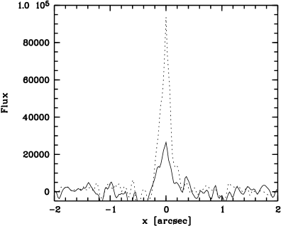
Figure 3: Deconvolved bulge$+$nucleus subtracted surface brightness profiles of the so-called “UV peak” in the nucleus of M 31 (WFPC2/HST) in $V$ (solid line) and $U$ (dashed line). Flux units are in $L_{\odot}$.pc^-2 in the corresponding band (corrected for galactic extinction).

It is surprising to see how well this simple decomposition procedure works: the only significant residuals in the $U$ band indeed come from the UV peak (also seen in the $V$ band) and from very blue (extreme horizontal branch?) stars clustering around the nucleus (Brown et al. Brown98 (1998)). This shows that our bulge model is adequate (keeping in mind that the exact bulge light contribution remains unknown in the central arcsecond). It accounts for the observed ellipticity and position angle of the isophotes in the central 20 arcseconds. It also confirms that the core of M 31 can indeed be decomposed into three distinct components: the bulge, the nucleus, including P1, and the UV peak. The obtained colours for the bulge and the nucleus are then (corrected for galactic extinction: $0.42$, $0.24$, and $0.1436$ mag in $U$, $V$ and $I$ respectively): $(V-I)_{B}=1.26$, $(U-V)_{B}=1.98$ and $(V-I)_{N}=1.30$, $(U-V)_{N}=2.36$. The UV peak has an average axis ratio of $\sim 0.7\pm 0.05$, a PA of $\sim 62\degr\pm 8$, a major-axis FWHM of $0\aas@@fstack{\prime\prime}21$, and has $(U-V)=-0.35$. We therefore find that the nucleus is redder than the bulge: this is in contradiction with the results of Lauer et al. (Lau98 (1998)) who found that the nuclear region is bluer than the bulge in the $U-V$ colour. We checked and confirm the robustness of this result by reexamining the original images. We thus cannot explain this discrepancy even considering the slight differences in the reduction process.

2.3 Centres and positioning

Following the photometric decomposition achieved in Sect. 2.2, we have chosen our reference centre, position $[0,0]$ throughout the paper, to correspond to the central UV maximum in the F300W image (see Fig. 3). This choice was motivated by the fact that the UV peak is very bright and just resolved in the WFPC2 images, allowing a very accurate determination of its centre. It is also thought to correspond to the true position of the presumed central massive black hole as discussed by KB99. KB99 defined their spatial zero radius $x_{\mbox{\tiny KB}}$ to be the velocity centre at the resolution of their SIS data. Comparing their surface brightness profile (their Fig. 8) with the F300W and F555W WFPC2 photometry, we find that $x_{\mbox{\tiny KB}}$ is $0\aas@@fstack{\prime\prime}031$ away (towards P1) from the position of the UV peak (our $[0,0]$). KB99 quoted a value of $0\aas@@fstack{\prime\prime}051\pm 0\aas@@fstack{\prime\prime}014$ between the UV peak and $x_{\mbox{\tiny KB}}$. This difference (of $0\aas@@fstack{\prime\prime}02$) is easily accounted by the fact that the contribution of the “UV peak” quickly decreases at longer wavelengths, the local maximum around P2 shifting away from P1, with an offset of about $0\aas@@fstack{\prime\prime}023$ already in the V band (roughly one dithered pixel). Throughout this paper, P2 is defined as the secondary surface brightness maximum in the $I$ band, where we assume that the UV excess has a negligible contribution. P2 is indeed not coincident with the location of the UV peak: it shows up (in the $I$ band) as an elongated structure, it centre being at about $0\aas@@fstack{\prime\prime}076$ from the UV peak (see Fig. 6).

The spatial zero radius of Statler et al. (Sta99b (1999), Sta+99) is about $-0\aas@@fstack{\prime\prime}025$ from the UV peak (away from P1), according to their approximate surface brightness long-slit profile (spectral domain from $\sim 4000$ to 5450 Å, see their Fig. 3). Their zero radius is therefore $0\aas@@fstack{\prime\prime}025+0\aas@@fstack{\prime\prime}031=0\aas@@fstack{\prime\prime}056$ from the one defined in KB99. However, careful inspection of Fig. 6 in Sta+99 shows that the kinematical data of KB99 has been uncorrectly shifted by $\sim 0\aas@@fstack{\prime\prime}13$ (towards P1) in order to be consistent with their FOC kinematics: this shift is then $\sim 0\aas@@fstack{\prime\prime}074$ larger than it should be. The fact that Sta+99 managed to roughly fit the kinematical data of KB99 comes partly from the way the extrapolation of their one-dimensional $V$ and $\sigma$ FOC profiles was achieved, assuming almost no dependency perpendicular to the slit (see Sect. 5.1 of Sta+99), and partly from this uncorrect spatial registering.

To summarize, the zero radius defined in Sta+99 and in KB99 are offset by $-0\aas@@fstack{\prime\prime}025$ and $0\aas@@fstack{\prime\prime}031$, respectively, with respect to our spatial zero point taken as the location of the UV peak in the F300W band (Fig. 6). We do not include here unknown (small) potential offsets perpendicular to their slits.

3 OASIS spectrographic data

3.1 Observations

We observed the nucleus of M 31 in December 98 using the OASIS integral field spectrograph attached to the CFHT adaptive focus bonnette (PUEO). OASIS is the successor of the TIGER integral field spectrograph successfully used at CFHT between 1987 and 1996. The instrument design follows the TIGER concept described in Bacon et al. (Bac95 (1995)), and includes a spectrographic mode, in which the spatial sampling is achieved via a microlens array, and an imaging mode. Various sampling sizes and spectral resolutions are available, from 0.04 arcsec to 0.16 arcsec per lens, and $400<R<4000$ respectively. OASIS has been designed and built at the Observatoire de Lyon and is operated at CFHT as a guest instrument.

We used the MR3 configuration covering the Ca triplet (8500 Å) region. This configuration was favoured against the classical Mg2 (5200 Å) wavelength range because PUEO, like all other adaptive optics systems, performs better at longer wavelength (Rigaut et al. Rig98 (1998)). The selected spatial sampling of $0\aas@@fstack{\prime\prime}11$ per (hexagonal) lens provides a field of view of 4$\times$3 arcsec². Details of the instrumental setup are given in Table 2.

A total of nine exposures, each 30 mn long, were obtained during a seven day period (December 17–24). The atmospheric conditions were photometric. Seeing conditions were generally good, but changed rapidly (see Sect. 3.2.2). All exposures were centred on the nucleus, with only small offsets (typically of the order of 1–2 sampling size). Neon arc lamp exposures were obtained before and after each object integration, and other required configurations exposures (bias, dome flatfield, micropupil) taken during daytime. Bright sky flatfields were also observed at dusk or dawn. The star HD 26162 (K2 III) was chosen as a kinematical template, and observed with the same instrumental setup.

Table 2: OASIS instrumental setup

PUEO
Loop mode	automatic
Loop gain	80
Beam splitter	I
OASIS
Spatial sampling	0.11 arcsec
Field of view	$4\times 3$ arcsec2
Number of spectra	1123
Spectral sampling	2.17 Å pixel-1
Instrumental broadening ($\sigma$)	69 km s-1
Wavelength interval	8351–9147 Å

3.2 Data reduction

The OASIS data were processed using the dedicated XOasis software (version 4.2) developed in Lyon. The standard OASIS reduction procedure includes CCD preprocessing (bias and dark subtraction), spectra extraction, wavelength calibration, spectro–spatial flatfielding, cosmic rays removal and flux calibration. Given the high surface brightness of the nucleus of M 31 and the small field of view, no sky subtraction was required.

3.2.1 Spectra extraction and calibration

The extraction of the spectra is the most critical phase of the reduction process. It uses a physical model of the instrument with finely tuned optical parameters, such as the rotation angle of the grating with respect to the CCD column, the tilt of the grism, the collimator and camera focal ratios, etc. The free parameters are fitted using a set of calibration exposures (micropupils – obtained without the grism –, arc and tungsten continuum frames) and saved in an extraction mask, later used to retrieve the precise (subpixel) location of each spectrum. Small shifts of the spectra location obtained at different airmass may occur due to mechanical flexures. These are corrected by including a global shift between the object exposure and the extraction mask. This offset is measured via the cross-correlation of the arc frame associated with the science exposure, and the one associated with the reference continuum exposure (used to build the extraction mask). Shifts are typically 0.1–0.2 pixel. Given that observations of M 31 were split over eight nights, we built two extraction masks from two sets of calibration exposures obtained at the start and end of the run respectively. These two masks were found to be almost identical, both giving an excellent fit (0.08 pixel RMS residuals between the model and the continuum exposure). Various extraction tests using each mask independently showed no significant differences, and we chose to use only the first mask. All spectra were extracted via an optimal extraction algorithm (Bacon et al. Bac01 (2001)) applied to each exposure (object and associated arcs), finally providing 9 science datacubes with 1123 spectra each.

These datacubes were then wavelength calibrated using the associated (nearest) arc exposure. The goodness of the optical model guarantees that the raw extracted spectra do already have a good wavelength precalibration. First order correction polynomials were thus sufficient to finalise the calibration, with typical RMS residual errors of 0.04–0.05 Å ($\sim 1.5$ km s^-1). After wavelength rebinning, the spectro-spatial flatfield correction was applied to each individual spectrum. This correction is obtained using a combination of a high S/N continuum datacube (tungsten lamp) and a twilight sky flat field datacube. The former is used to correct the spectral variations, while the latter allows to correct lens-to-lens flux variations. Cosmic rays are then detected via a comparison beween each spectrum and its neighbours, and removed. The overall fraction of pixels affected by cosmic rays is small, typically 0.2–0.3%. Finally, spectra are truncated to a common wavelength range (8361–8929 Å) covering the Ca absorption line triplet. No flux calibration was performed, since this is not required to measure the stellar kinematics.

3.2.2 PSF determination, and merging of the datacubes

PSF determination deserves special attention. Indeed, a precise knowledge of the spatial PSF is critical to be able to compare in detail datasets which span a rather large range in spatial resolution (from HST to ground-based long-slit observations).

Reconstructed images are computed by direct summation of spectra along the wavelength range followed by an interpolation on a square grid. As expected, the 9 reconstructed images present significantly different PSFs. We used the available HST/WFPC2 $I$ band images of the M 31 nucleus (see Sect. 2) to have an accurate estimate for each of them. Assuming a parametric shape for the PSF, we performed a simple least-squares fit between the convolved HST image and the equivalent reconstructed OASIS image. Free parameters for the fit also include the relative alignement and rotation between the two images, as well as the corresponding flux normalisation factor.

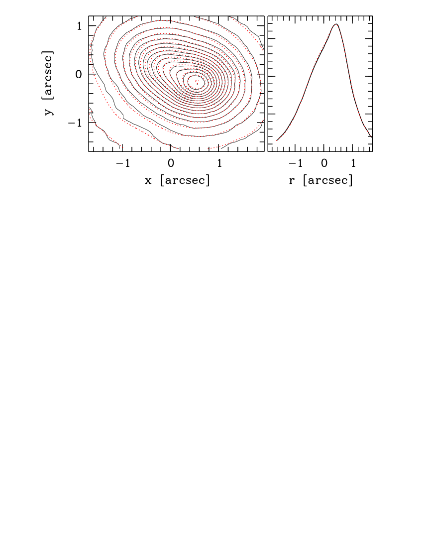
Figure 4: PSF fitting of OASIS exposure #6. Left panel: Contour plot of the reconstructed image (solid line) and the convolved HST image (dashed line). Right panel: photometric major-axis cut.

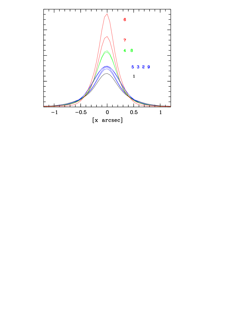
Figure 5: Fitted PSF of the nine OASIS exposures. FWHM range from 0$\aas@@fstack{\prime\prime}$79 (exposure #1) to 0$\aas@@fstack{\prime\prime}$39 (exposure #6)

Table 3: PSF parameters of the merged exposures

ID	Exp.	FWHM	$\sigma_{1}$	$\sigma_{2}$	$I_{2}/I_{1}$	$\sigma_{3}$	$I_{3}/I_{1}$
M2	6 – 7	0.41	0.15	0.29	0.98	0.448	0.023
M8	2 – 8	0.50	0.18	0.35	1.07	0.407	0.030

The reference HST/WFPC2 F814W ($I$) band filter covers a wavelength range which extends well beyond the spectral limits of the OASIS datacubes. However, colour gradients in the M 31 nucleus are very small in the visible, so we decided to neglect the effects due to the differences in the response curve: we checked that this had a negligible effect on the final PSFs parameters. The PUEO adaptive optics performance heavily depends on the “original” seeing conditions, the brightness of the guiding source and the wavelength range. OASIS observations of the M 31 nucleus are thus challenging for PUEO, given the low contrast and complex structure in the M 31 nucleus, and the relatively blue wavelength range of the observations (compared to the more classical near-infrared H or K bands). Typical PUEO PSFs at these wavelengths are not diffraction limited, but show a core of a few tenths of an arcsec surrounded by a large halo. A sum of $3$ gaussian functions provides a reasonable approximation. An illustration of the quality of the fit is given in Fig. 4. This procedure does not only provide PSF parameters but, as mentioned above, also the precise relative centring between the OASIS exposures and the HST/WFPC2 image.

All nine computed PSFs are displayed in Fig. 5. There are large differences in the resolutions of the nine exposures, which range from 0$\aas@@fstack{\prime\prime}$79 to 0$\aas@@fstack{\prime\prime}$39 FWHM. Two merged exposures have thus been created using two different sets of exposures ranked according to their resolution:

• the first one, hereafter called M2, with the highest spatial resolution is the combination of exposure #6 and #7 only.

• the second one, hereafter called M8, with a higher S/N but a corresponding lower spatial resolution, is the combination of all exposures except exposure #1.

The selected datacubes were merged using the accurate centring given by the PSF fitting procedure. Interpolation on a common square grid is performed before averaging the data. One lens located in the outer part of the nucleus was affected by a bad CCD column and was discarded before interpolation. The PSF fitting was subsequently performed on the merged datacube and the results are given in Table 3. The M2 and M8 exposures have cores FWHM of $0\aas@@fstack{\prime\prime}34$ and $0\aas@@fstack{\prime\prime}41$ respectively, both with extended wings giving a global FWHM of $0\aas@@fstack{\prime\prime}41$ and $0\aas@@fstack{\prime\prime}50$ respectively.

3.2.3 Computation of line-of-sight stellar velocity distributions

A velocity template spectrum was obtained using the reference star HD 26162 datacube, summed over an aperture of $1\arcsec$ to maximize the S/N. The spectrum was then continuum divided and rebinned in ln($\lambda$). The same procedure was applied to the merged datacubes of M 31. We used the Fourier Correlation Quotient (FCQ) method, originally developed by Bender (Bender90 (1990)), to derive the kinematical maps. The kinematics was parametrized using a simple Gaussian and complemented using third and fourth order Gauss-Hermite moments (van der Marel & Franx vdMF93 (1993)). All velocities were offset to heliocentric values. A systemic velocity of $308$ km s^-1 was deduced by comparing our data to the data of KB99 whose kinematics extends far enough to observe the slow rotation of the bulge (see Sect. 5).

3.2.4 Bulge subtraction

Since we are mostly interested in the kinematics of the nucleus of M 31, we would like to subtract the contribution of the bulge from the OASIS merged datacubes. This was performed using the photometric model derived in Sect. 2.2 (see KB99 for a similar approach). We extracted a mean bulge spectrum from the outer part of the OASIS field, which we fitted making use of a library of stellar templates to get a high S/N reference spectrum. We then used a simple Jeans dynamical model (see Emsellem et al. Ems94 (1994)) to derive the velocity and velocity dispersion of the bulge (taking into account the instrumental setup and seeing) in the OASIS field of view. The resulting spectra were finally directly subtracted from the OASIS datacubes (M2 and M8) after the proper luminosity normalisation. We checked that slight variations in the continuum shape or absorption line depths did not produce any significant differences on the final bulge-subtracted datacube spectra. The results do however weakly depend on the details of the dispersion model used for the bulge: the same subtraction procedure was therefore also applied using a constant dispersion of 150 km s^-1  for the bulge. The difference comes mainly from the higher assigned central dispersion to the bulge in the Jeans model. In Sect. 5.2, we will only discuss results from the bulge-subtracted M8 OASIS datacube, which has a significantly better S/N.

4 STIS/HST data

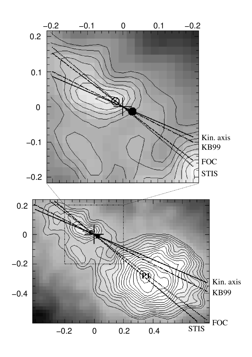
Figure 6: The central region of the deconvolved WFPC2 image in the $I$ band showing the location of P1, P2 and the UV peak. Isophotes are drawn from 11.79 to 12.49 with a step of 0.05 mag arcsec^-2. The UV peak, located at $[0,0]$, is marked by a cross. The solid line represents the kinematical major-axis, with which P2 elongation is well aligned. The slit axis for the SIS (KB99), STIS  (this paper) and FOC (Sta+99) data are represented by dotted-dashed, dashed and dotted lines, respectively. The filled and empty circles represent the location of the spatial zero point of the SIS and FOC long-slit data, respectively. The upper panel shows a zoom in the central $0\aas@@fstack{\prime\prime}2$. Note the distance between the maximum of P1 (marked with the text ”P1”) and the kinematical major-axis.

The nucleus of M 31 was observed with STIS at PA$=39\degr$ in July 1999, using the G750M grating and the $52\times 0\aas@@fstack{\prime\prime}1$ slit (Proposal 8018, PI Green). The spatial pixel was $0\aas@@fstack{\prime\prime}05071$, and the velocity resolution about 38 km s^-1. We have retrieved the 8 corresponding science exposures and calibration files from the ST/ECF archives in this configuration. After the data reduction provided via the ST/ECF pipeline using the best reference files, we corrected the individual frames for the residual fringing using the dedicated routines available under IRAF (Goudfrooij & Christensen Gou98 (1998)) and the available contemporaneous flat fields. We combined the individual exposures after careful recentring, and extracted individual spectra, which were rebinned in $\ln{(\lambda)}$ for the kinematical measurements. The spatial centre of the long-slit luminosity profile was then accurately determined taking the same reference zero point as in the WFPC2/HST data (see Sect. 2.3). Spectra were binned along the slit to increase the S/N outside $0\aas@@fstack{\prime\prime}85$ from the centre. We also retrieved STIS exposures from the K0III star HR 7615 (same configuration) from the archive to be used as a stellar template, and reduced them in the same way. The line-of-sight velocity distribution at each spatial location was finally derived using the Fourier Correlation Quotient method as in Sect. 3.2.3. We estimated a maximum velocity error of $\sim 8$ km s^-1 due to the slit effect using the present STIS characteristics (see Bacon et al. Bac95 (1995)). In the present paper, we will mainly focus on the first two moments, namely the velocity and velocity dispersion, only using the higher order Gauss-Hermite moments to derive an estimate of the first two true velocity moments. We finally performed the subtraction of the contribution of the bulge as in Sect. 3.2.4.

5 Results

5.1 OASIS stellar velocity maps

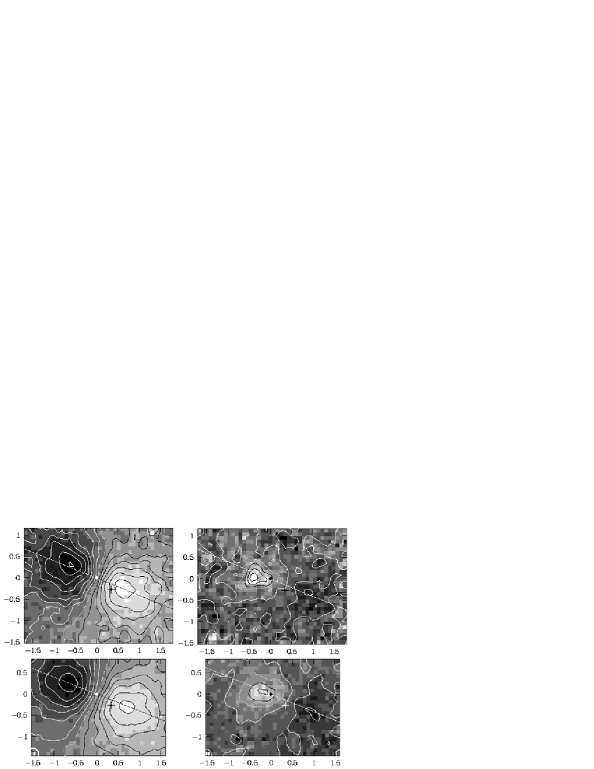
Figure 7: OASIS stellar kinematical maps: stellar velocities (left panels) and dispersions (right panels). The top and bottom panels correspond to the high spatial resolution datacube (M2) and the high S/N datacube (M8), respectively. The dotted white lines display the zero isovelocity contour and the 200 km s^-1  isovelocity dispersion. The step is 25 km s^-1  in all panels. The centre of the UV peak, our $[0,0]$, is marked by a filled circle, the cross marking the centre of P1. The dashed lines indicate the kinematical major-axis. North is at a PA of $192\degr$, East at its right, and the scale is in arcsecond.

In Fig. 7, we present the stellar velocity and velocity dispersion maps for the two final datasets M2 and M8. Both give similar results, as shown in Fig. 8, although the difference in spatial resolution can be seen in the central velocity gradient and velocity dispersion peak.

We compare these results with the KB99 kinematical profiles obtained with the SIS/CFHT spectrograph at a spatial resolution of $0\aas@@fstack{\prime\prime}65$ FWHM. The SIS slit position has been spatially shifted by $+0\aas@@fstack{\prime\prime}031$ to account for the small offset between the location of the UV peak and the velocity centre as defined by KB99 (see Sect. 2.3). A simulated OASIS slit was computed using the surface brightness weighted average of the kinematical quantities ($V$ and $\sqrt{V^{2}+\sigma^{2}}$) over an equivalent slit opening of $0\aas@@fstack{\prime\prime}35$ at PA$=52.5\degr$ (Fig. 9). The comparison was done using the M8 data set. The agreement is excellent, with 8 and 9 km s^-1  RMS residual in velocity and velocity dispersion, respectively. Note that the difference due to spatial resolution is largely smoothed by the averaging over the 0$\aas@@fstack{\prime\prime}$35 slit width.

The precise axis and centre of symmetry of the velocity field was estimated using a fit with a simple analytical function. In that model, the velocity field was parametrized as a sum of first order Gauss-Hermite-like functions $x^{\prime}\cdot\sum_{i}\;\mathrm{Gauss}_{i}(x^{\prime},y^{\prime})$ where $x^{\prime},y^{\prime}$ are cartesian coordinates on the sky. Free variables are the coordinates of the individual centres ($x_{0}^{i},y_{0}^{i}$), the principal axis angle ($\theta_{0}$), the Gaussian parameters ($\sigma_{i},I_{i},q_{i}$) and a zero velocity. Experiments show that the kinematic centre and tilt are insensitive to the details of the fitting functions provided it is antisymmetric. The two merged datacubes gives consistent results. A use of only two components provides a reasonable fit with 16 km s^-1  RMS residuals. The centre of symmetry is found at [0,0] within 20 mas and the kinematic axis with $\theta_{0}=56.4\pm 0.2\degr$. The velocity at [0,0] is not zero, but $\sim-9$ km s^-1.

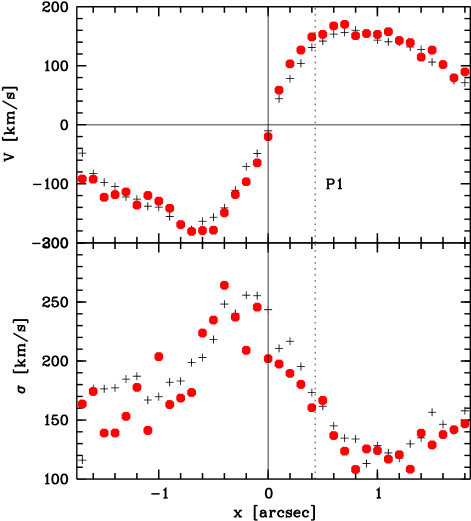
Figure 8: OASIS velocity profiles along the kinematic axis (PA$=56.4\degr$, averaged over a width of $0\aas@@fstack{\prime\prime}2$). Top panel: stellar velocity. Bottom panel: stellar velocity dispersion. The crosses and circles correspond to the high S/N (M8), and the high spatial resolution (M2) datacubes respectively.

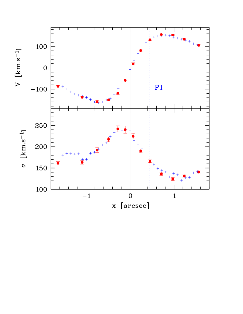
Figure 9: Comparison between the SIS kinematics (circles; Kormendy & Bender KB99 (1999); PA$=52.5\degr$, slit width of $0\aas@@fstack{\prime\prime}35$) and the OASIS equivalent slit (crosses). Top panel: mean velocity. Bottom panel: velocity dispersion.

The kinematic axis is significantly different from the P1–P2 axis (PA $42\degr$) as shown in Fig. 7, and P1 is offset $0\aas@@fstack{\prime\prime}12$ from the kinematic axis. The fact that P1 is not aligned on the kinematic major-axis must be taken into consideration for the interpretation of the high spatial resolution HST kinematical data which have been taken close to the P1–P2 axis.

The velocity dispersion map of the (best resolved) M2 datacube peaks at 270 km s^-1  at $0\aas@@fstack{\prime\prime}3\pm 0\aas@@fstack{\prime\prime}1$ on the anti-P1 side. The peak is extended, and surrounded by a halo which itself extends above the nearly constant bulge velocity dispersion of $\sim 150$ km s^-1. The same structure is found in the M8 datacube, but with a lower contrast. The dispersion is clearly asymmetric with respect to the UV peak, with a difference of 35 km s^-1  at $\pm 1\aas@@fstack{\prime\prime}2$ along the kinematic axis. Note that the offset of the velocity dispersion peak is also present in the KB99 data (see their Fig. 4). The small difference is simply due to the slightly lower resolution of the SIS data (including the smoothing onto the $0\aas@@fstack{\prime\prime}35$ arcsec slit width). Such an offset was also present in the TIGER data (Bacon et al.Bac94 (1994)), but with a larger value ($0\aas@@fstack{\prime\prime}7$), due to the lower spatial resolution ($0\aas@@fstack{\prime\prime}9$ FWHM).

5.2 Bulge-subtracted velocity maps

We have used two different models for the (unknown) velocity dispersion of the bulge: a constant value of 150 km s^-1, or the dispersion predicted by a simple Jeans model using the combined gravitational potential of the nucleus and the bulge (as in Bacon et al. Bac94 (1994)). The two resulting kinematical profiles only show minor differences, the bulge-subtracted velocity and dispersion for the ”constant dispersion” model being slightly larger: for clarity, we will only deal with the latter (note that these profiles are consistent with the bulge-subtracted kinematics of KB99).

After the subtraction, the asymmetry in the velocity field is now clear, with the anti-P1 side having a slightly higher velocity amplitude with a local minimum at $-250$ km s^-1  (at $\sim 0\aas@@fstack{\prime\prime}75$ from the centre; fig. 10). The velocity profile on the P1 side is nearly flat with a value of $\sim 180$ km s^-1. The dispersion now peaks at 329 km s^-1  at $-0\aas@@fstack{\prime\prime}1$ from the centre. We also confirms that the nucleus is cold (KB99), with a value of $108\pm 10$ km s^-1 at $1\aas@@fstack{\prime\prime}2$ along the kinematical major-axis on the P1 side.

Figure 10: Bulge-subtracted OASIS kinematics along the kinematic major-axis of the nucleus compared with the original OASIS M8 profiles (crosses). The solid line shows the resulting kinematics when using a constant dispersion of 150 km s^-1  for the bulge, and the dotted line when using the dispersion predicted by a simple Jeans model.

5.3 STIS and FOC kinematical profiles

The STIS velocity and dispersion profiles are presented in Fig. 11. There is a clear asymmetry in the velocity curve, with local turnover values of $197\pm 5$ and $-292\pm 20$ km s^-1  at radii of $+0\aas@@fstack{\prime\prime}42$ and $-0\aas@@fstack{\prime\prime}235$ respectively. The maximum velocity on the P1 side is $201\pm 5$ km s^-1  at $0\aas@@fstack{\prime\prime}63$. The dispersion is maximum on the anti-P1 side at a radius of $-0\aas@@fstack{\prime\prime}235$ with a value of $321\pm 33$ km s^-1  (and a value of $313\pm 36$ km s^-1  at $-0\aas@@fstack{\prime\prime}18$). This is to be compared with the offset of $0\aas@@fstack{\prime\prime}15$–$0\aas@@fstack{\prime\prime}20$ found by KB99 and $\sim 0\aas@@fstack{\prime\prime}2$ for the slit profile reconstructed from the OASIS data. The STIS velocity profile crosses the $V=0$ line at $+0\aas@@fstack{\prime\prime}09$ (P1 side). At $[0,0]$ we measure $V=-68\pm 6$ km s^-1. After subtraction from the bulge contribution, the central velocity gradient is slightly steeper, with turnover values of $-355$ km s^-1 and $221$ km s^-1 at $-0\aas@@fstack{\prime\prime}235$ and $0\aas@@fstack{\prime\prime}47$ respectively.

Figure 11: STIS kinematical profiles: velocity (top panels) and dispersion (bottom) panels at a PA of 39$\degr$. The inserted panels present the STIS kinematical profiles within a radius of 10″.

Figure 12: Comparison between STIS (solid line) and FOC kinematics (filled triangles). A shift of $0\aas@@fstack{\prime\prime}025$ towards the anti-P1 side was applied, following the analysis made in Sect. 2.3. A positive shift of $30$ km s^-1 was applied to the FOC velocity profile (top panel, see text)

. The STIS data and the FOC data were taken at PAs of 39$\degr$ and 42$\degr$ respectively.

Comparing the original FOC (Sta+99) and the STIS data, we find significant discrepancies in both the velocity and dispersion profiles at the very centre which seem difficult to attribute to differences in instrumental characteristics. The most surprising difference is the location of the dispersion peak in the original FOC data which is nearly centred with an offset of only $0\aas@@fstack{\prime\prime}06$ from the UV peak (away from P1). By including the observed spatial shift of $0\aas@@fstack{\prime\prime}025$ mentioned in Sect. 2.3, as well as a velocity shift of $30$ km s^-1, the comparison looks reasonable (Fig. 12): this point is discussed below (Sect. 5.4).

5.4 OASIS compared with HST kinematics

Although the STIS and FOC data have similar slit widths (0$\aas@@fstack{\prime\prime}$1 for STIS and 0$\aas@@fstack{\prime\prime}$063 for FOC) and PAs ($39\degr$ for STIS and $42\degr$ for FOC), the FOC data (Sta+99) have been obtained at much bluer wavelengths than STIS (0.45 versus 0.85 $\mu$m) and have a better spatial resolution (Fig. 12). A detailed comparison between the STIS and FOC data sets thus requires to take into account these specific characteristics. But this implies the convolution of the (yet unknown) 2D kinematics of M 31 at FOC spatial resolution. We also wish here to compare HST and OASIS kinematical data: the two-dimensional coverage of the OASIS spectra is in this context a powerful additional constraint. The comparisons between the OASIS and STIS datasets are shown in Fig. 13.

Figure 13: Comparison between the kinematics from STIS (crosses) and OASIS (filled circles). The OASIS kinematics have been averaged over a $0\aas@@fstack{\prime\prime}2$ wide slit (PA$=39\degr$).

To attempt such a comparison, we have built simple 2D parametric kinematical models. These models are obviously ill-constrained, given that we have knowledge on only a tiny fraction (2.5%) of the area covered by OASIS at FOC resolution, and do not stand on any physical ground. This ad hoc model is solely designed to check if the three kinematical data sets are consistent with each other, i.e. if we can find a reasonable model which simultaneously fits all the observed kinematics. All convolutions are achieved taking into account the relevant pixel integration. The surface brightness distributions were derived from the deconvolved WFPC2 images: we kept the F814W filter image for both the STIS and OASIS data, and used a weighted sum of the F300W and F555W images to roughly reproduce the surface brightness profile of the FOC data presented by Sta+99. In the cases of the OASIS and STIS data, we used an estimate of the first two true velocity moments (the best gaussian velocity and velocity dispersion depending on the shape of the line-of-sight velocity distribution). For the FOC data, we had to use the original values as published by Sta+99. Since Sta+99 mention that the kinematics derived from the half blue and red parts of their spectra are indistinguishable, we assumed in the following that the UV peak does not contribute to the kinematical profile. In other words, we assumed that the stars forming the UV peak do not show (metallic) features strong enough to significantly contribute to the observed kinematics: this hypothesis seems to be supported by a preliminary analysis of the STIS/G430L data (Emsellem et al., in preparation).

Figure 14: Comparison of OASIS (left), STIS (middle) and FOC (right) kinematics within the central arcsec. Velocity and dispersion profiles are shown in the bottom and top panels respectively. Original FOC data (right panels) have been shifted by $0\aas@@fstack{\prime\prime}025$ and $30$ km s^-1 (see text). The solid lines represent the model convolved and sampled according to the corresponding instrumental setup.

Figure 15: Same as in Fig. 14 but for the OASIS and STIS data in the central 2″.

We start with a model based on velocity functions of a simple form $V(r)=K\cdot x\cdot(1+r^{2}/r_{e}^{2})^{-n}$ with $r^{2}=x^{2}+y^{2}/q^{2}$ ($x$ and $y$ being the cartesian coordinates aligned with the kinematical axis), and constant or gaussian functions for the velocity dispersion. The PA of the kinematical major-axis was set to 56.4$\degr$ as measured from the OASIS data. The observed asymmetries in the kinematical profiles were obtained by allowing both spatial and velocity offsets in the parametrized functions. We fixed the dispersion of the bulge and the nucleus to 150 km s^-1  and 108 km s^-1 respectively, adding (quadratically) a gaussian of $1\aas@@fstack{\prime\prime}2$ FWHM with a maximum of 140 km s^-1 located at $0\aas@@fstack{\prime\prime}8$ on the P1 side to reproduce the low-frequency spatial asymmetry seen in the OASIS dispersion map (Fig. 7). The velocity and the non-centred second order moment ($V^{2}+\sigma^{2}$) are then convolved, after proper luminosity weighting. The input parameters were tuned until a satisfactory result was obtained.

The best overall fit was obtained by adding high velocity components in the central $0\aas@@fstack{\prime\prime}3$ aligned with the kinematic major-axis. The dispersion peak then simply results from the effect of velocity broadening as shown in Fig. 15. We cannot distinguish between a velocity broadening effect from true velocity dispersion of components that are spatially unresolved. This model is anyway the simplest we found which provides a reasonable fit to the STIS and OASIS data. It includes maximum amplitude velocities of $\sim+235$ and $\sim-265$ km s^-1 (outside the central $0\aas@@fstack{\prime\prime}3$). We also confirm the spatial and velocity offsets in the original FOC data with respect to the UV peak and the zero velocity as measured by KB99, respectively: by shifting the FOC kinematics by $0\aas@@fstack{\prime\prime}025$, consistently with the analysis of Sect. 2.3, and adding 30 km s^-1 to their systemic velocity, we can indeed reconcile the model with the FOC data (Fig. 14). Note that this velocity shift is consistent with the maximum possible systematic error of $50$ km s^-1  quoted by Sta+99. The high velocity component of the model is an attempt to reproduce the abrupt jump seen in the FOC rotation curve at a radius $\sim-0\aas@@fstack{\prime\prime}1$, near the location of the dispersion peak. This feature should however not be overinterpreted, although we believe that the central dispersion peak can indeed be explained via velocity broadening with the contribution of fast moving stars within $0\aas@@fstack{\prime\prime}3$ of the UV peak on the anti-P1 side. We do not find any significant discrepancy in the dispersion profiles contrarily with what was advocated by Sta+99: as mentioned earlier (Sect. 2.3), they uncorrectly shifted KB99’s data to manage a consistent fit (their Fig. 6).

We cannot make any definite statement about the detailed kinematics in the central $0\aas@@fstack{\prime\prime}3$, as there is too much freedom in the model parameters. This is mainly due to the fact that FOC and STIS provide only one-dimensional profiles, unlike OASIS data which are two-dimensional, but have a too low spatial resolution to constrain the dynamics at that scale. We can however still make a few relatively safe statements, which will be discussed further in Sect. 7:

• The observed kinematics is definitely not consistent with a dispersion peak at the location of the UV peak (our $[0,0]$).

• The dispersion peak and high velocities seem to be spatially associated with P2 (as seen in the $I$ band) which is offset from the UV peak on the anti-P1 side as shown in Fig. 6.

• The OASIS, STIS and FOC kinematical profiles are consistent with each other, although a two-dimensional coverage of the central $0\aas@@fstack{\prime\prime}3$ is required to properly address the kinematics there.

6 Numerical Simulations

We now interpret the observations with the help of N-body modeling. Among the various hypothesis that have been advanced to explain the M 31 double nucleus (with luminosity peak P1 shifted by $\sim$ 1.8 pc from the kinematical centre, almost coinciding with the UV peak), the most natural would be an $m=1$ wave in a rather cold and thin disk orbiting the SBH, located at the centre of the UV peak. The disk has to be cold, to be unstable to non-axisymmetric waves, and this implies a small thickness, in the almost spherical potential provided by the central SBH. However it is still unclear whether $m=1$ perturbations, accompanied by a displacement of the gravity centre, will be unstable, and develop spontaneously in the physical conditions corresponding to the M 31 nucleus (Heemskerk et al. Hee92 (1992), Lovelace et al Lov99 (1999)).

An alternative solution is that the disk is initially perturbed by an external force (either a globular cluster or Giant Molecular Cloud passing by), and the response is long-lived with a time-scale comparable to that of such external perturbations. We have simulated this possibility, and indeed found modes of $m=1$ oscillations that maintained during 70 Myr, with an almost constant pattern speed. This peculiar feature is due to the very low precession rate in an almost Keplerian disk, near a SBH. The asymmetry of the density, and the radial variation of eccentricity of the orbits, generate local variation of the effective precession rate, and most of the stars are dragged into a mode of slow, positive pattern speed. In this paper, we propose that this mechanism is at the origin of the M 31 $m=1$ perturbation (or “double-nucleus” morphology), and illustrate this with N-body simulations with asymmetric initial conditions. We consider in a future work the possibility that the $m=1$ instability develop spontaneously from axisymmetric initial conditions (Combes & Emsellem CE01 (2001)).

6.1 N-body Methods and Diagnostics

We performed essentially 2D simulations, since our interpretation is that the nuclear disk of M 31 is cold and thin (axis ratio of the order 0.1). The apparent axis ratio must then be mostly due to an inclination of $i\sim 55^{\circ}$ (see Sect. 6.3), less edge-on than the large-scale M 31 disk ($i=77^{\circ}$). However we also checked the results with 3D experiments. The gravity is solved via fast Fourier Transforms, on a useful 2D grid of $256\times 256$ ($512\times 512$ to suppress Fourier images). In 3D, the N-body code is a FFT scheme, which uses the James (Jam77 (1977)) method to avoid the influence of Fourier images. The grid is then $128\times 128\times 64$. The size of the simulated box in the disk plane is 20 pc, corresponding to a cell size of 0.078 pc (and twice that in 3D). This size is also the softening length of the Newtonian gravity. The M 31 nuclear stellar disk is represented in 2D by 99000 particles and 152384 in 3D. Two rigid potentials are added, representing the bulge and the supermassive black hole. The time step is 10^-4 Myr.

Particle plots are made in face-on and M 31-sky projections, together with the velocity field, the density, velocity and dispersion profiles along the major axis, to compare with the observed quantities (with and without bulge addition). The Fourier analysis of the density and potential are made regularly as a function of time and radius. If the potential is decomposed as $\Phi$(r,$\theta$) = $\Phi_{0}$(r) + $\Phi_{m}$(r) cos (m $\theta$ - $\phi_{m}$), we define the intensities of the various components by their maximal contribution to the tangential force, normalised by the radial force $F_{r}=-\partial\Phi_{0}/\partial$r, through

$$S_{m}=m\Phi_{m}/r|F_{r}|$$

In some simulations the SBH is allowed to move, with respect to the fixed background bulge. However, this introduces additional oscillations, of small amplitude, which are not well computed with the low spatial resolution in 3D. Therefore in most cases, the SBH was fixed at the centre of the bulge. These oscillations are of different (higher) frequencies that the phenomenon we are studying here, and are only superposed to it. They may be related to the nuclear oscillations studied by Taga & Iye (Tag98 (1998)) and Miller & Smith (Mil92 (1992)).

Over all run periods of typically 10-100 Myr, the Fourier analysis of the disk potential was done as a function of radius, and stored every 0.03 Myr. The result $F(r,t)$ is then Fourier transformed in the time dimension, in order to get the power as a function of pattern speed, $\tilde{F}(r,\Omega)$. With respect to the frequency of the $m$ perturbation, the pattern speed is $\Omega=\omega/m$.

6.2 Galaxy Model and Initial Conditions

The massive black hole potential was softened to a few cell sizes to avoid prohibitively small values of the time step in the centre. It is represented by a Plummer shape potential,

$$\Phi_{BH}(r)=-{{GM_{\rm BH}}\over{\sqrt{r^{2}+r_{bh}^{2}}}}$$

with $r_{bh}=0.07$ pc. The mass of the SBH $M_{\rm BH}$ was varied between 3.5 and 10 10⁷ M_⊙ to test the role of the self-gravity of the disk. The fixed analytical potential of the bulge is composed of 4 Plummer functions, determined from the MGE method (see Emsellem & Combes EC97 (1997)). Their corresponding masses and radii are displayed in Table 4. The total mass of the bulge inside 9 pc is 0.87 10⁷ M_⊙. The nuclear stellar disk is initially a Kuzmin-Toomre disk of surface density

$$\Sigma(r)=\Sigma_{0}(1+r^{2}/d^{2})^{-3/2}$$

truncated at 9 pc, with a mass of $M_{d}=1.7\,10^{7}$ M_⊙, and characteristic radius of $d=3.5$ pc. It is initially quite cold, with a Toomre Q parameter of 0.3. The mass fraction of the disk inside 9 pc was varied between 20 and 40%.

Since the potential of the black hole is significantly smoothed below a radius equal to 2.5 times the softening length, here $2.5\times 0.07$ pc$=0.175$ pc, we have avoided putting particles in this region, so as not to introduce artificial dynamics. The initial surface density was then equal to the difference between two Toomre disks of the same central surface density, but different characteristic lengths. This was done to have an analytic density-potential pair with a smooth boundary for the central hole. Up to 12% of the central disk mass was thus removed and redistributed on the remaining outer parts. The exact value of the scale-length of the removed disk, between 0.5 and 1.2 pc, was of no importance on the final results. It is somewhat larger than the required 2.5 softening lengths, since the initial orbits near the black hole are eccentric, with a small pericentre. The potential inside this radius is in any case dominated by the keplerian law of the black hole, so that the suppression of the central stellar disk does not affect the rotation curve. The rotation curve obtained is plotted in Fig. 16.

Table 4: Parameters of the mass model

Component	Size	Mass∗
	pc	107 M⊙
SBH	0.07	7
Disk	3.5	1.7
Bulge-1	700	0.01
Bulge-2	160	0.07
Bulge-3	50	0.2
Bulge-4	15	0.6

^∗ mass inside 10 pc radius

The initial $m=1$ perturbation was produced in several ways: either the SBH position was shifted by an arbitrary value from the centre of the potential, or its velocity was perturbed and given a high value. In both cases, a long-lived $m=1$ pattern was obtained. However, the initial conditions were too far from equilibrium, and the violent relaxation led too many particles to escape. A softer way to perturb the disk is to launch particles in eccentric orbits from the start, keeping the SBH fixed at one of the foci of the elliptical orbits. Once a profile of eccentricity is chosen, each particle is moved along the corresponding ellipse at a random position with probability inversely proportional to its linear velocity at this point (probability density along the ellipse proportional to $1-e\cos{(\xi)}$, $\xi$ being the true anomaly). About 20 models were run, to investigate the nature of the modes, and the influence of initial conditions, the mass fraction of the disk, etc. The best fit for M 31 is described here, and compared with observations.

Figure 16: The observed orbital velocity $V$ (full line, in km/s), log of surface density in arbitrary units ($\Sigma$, dash), and radial velocity dispersion ($\sigma_{v}$, dot-dash), at the epoch of 54 Myr, for the galaxy model with $M_{\rm BH}=7\,10^{7}$ M_⊙.

6.3 Results

The best fit model for M 31 was obtained through the initial distribution of eccentricity

$$e(a)=0.6\sqrt{(1-(a/4\;\mathrm{pc})^{2})}$$

and $e(a)=0$ for $a>4pc$ ($a$ being the semi-major axis). The major axis of the orbits are initially aligned, but they quickly re-arrange, so that the pericentre of orbits in the inner and outer parts are in phase opposition. The face-on view of the nuclear disk is displayed in Fig. 18. There is a clear density accumulation on one side of the BH. The strength of the $m=1$ and $m=2$ Fourier components of the potential are plotted in Fig. 19, together with the position of the stellar disk gravity centre, as a function of time. At the beginning, until 15 Myr, there is a settling phase, where the $m=1$ mode has a trailing, than clearly leading arm. The stellar gravity centre precesses in the positive direction, and also the pattern speed in the power spectrum is positive (see Fig. 17). Then, the motion of the gravity centre becomes more regular, slows down slightly, with a period of 2 Myr, corresponding to a pattern speed of the $m=1$ perturbation of $\Omega_{p}\sim 3$ km/s/pc (the pattern speed is equal to the orbital frequency of the gravity centre). Note that the $m=2$ perturbation is just the harmonic of the $m=1$, and has the same pattern speed.

These values of pattern speed are about 10 times smaller than the value derived by Sambhus & Sridhar (2000) using the Tremaine-Weinberg method and M 31 FOC data. Note however that the latter method is rather uncertain when applied to one-dimensional data.

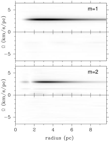
Figure 17: Pattern speed as a function of radius, in units of km/s/pc, for the $m=1$ mode (top) and the $m=2$ mode (middle) between the epochs 28.8 and 43.2 Myr ($M_{\rm BH}=7\,10^{7}$ M_⊙). The pattern speed slows down slightly with time, which thickens the lines (from 3 to 2.5 km/s/pc in 60 Myr).

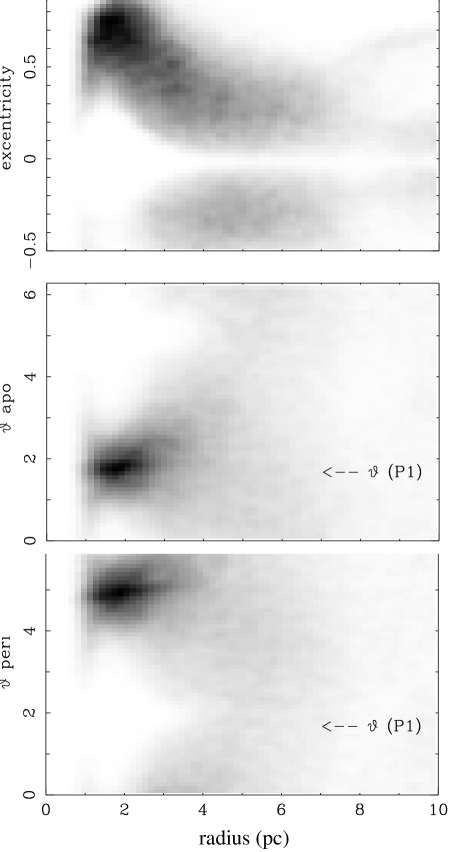
Figure 22: Eccentricity $e(a)$ of particles as a function of their major axis $a$ (top); $e(a)$ is counted positive when the apocentre is in the region of the P1 accumulation, negative otherwise. Polar angle (from the BH) $\theta_{apo}$ of the apocentre of orbits (middle), and $\theta_{peri}$ of their pericentre (bottom), at epoch 28.8 Myr. The position of the maximum density (corresponding to the P1 component of M 31) is indicated.

The distribution of eccentricity is quite similar all over the run, and typically represented by Fig. 22. It is always decreasing from $a=1$ pc to 6 pc, with a large scatter. The eccentricity is maintained at large values, and the apocentres are aligned to give the density accumulation that will give rise to P1 in M 31 (see the position of P1 in the middle and bottom of Fig. 22). From 5 to 10 pc, the apocentres change side, and there is a secondary density accumulation, in phase opposition with S1, of much smaller amplitude. The accumulation is also at the apocentre of these outer particles. The density accumulation is located very close to the maximum eccentricity gradient. As noted by Statler (Sta99a (1999)), this is a configuration that allows the right impulses on eccentric orbit to equalize the precessing rates. If an orbit grazes from the inside a density accumulation, the experienced outward pull can accelerate in the positive sense its precession, if it is at apocentre. If it is at pericentre, its precession will be slowed down. The nearly axisymmetric (epicyclic approximation) precessing rate is only slightly negative, and this small impulse is sufficient to align the orbits, and make them precess in the positive sense. The orbits should be at their apocentre inside the density peak, and at their pericentre inside, for the precessing corrections to go towards equalization. This explains the orbit orientation observed, and the fact that the two density accumulations are in phase opposition.

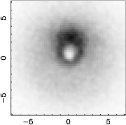
Figure 18: Face-on surface density of the nuclear stellar disk, at epoch 28.8 Myr ($M_{\rm BH}=7\,10^{7}$ M_⊙). The scale is in pc. The hole in the centre is introduced on purpose in the initial conditions, to avoid artificial effects due to the black hole softening and limited spatial resolution (see Sect. 6.2).

Figure 19: top: Coordinates (X: full line) of the centre of gravity of the stellar disk, as a function of time (model with $M_{\rm BH}=7\,10^{7}$ M_⊙). Note that the period is slightly increasing with time, i.e. the pattern speed slows down. bottom: Intensity of the $m=1$ (S1, solid line) and $m=2$ (S2, light line) Fourier components of the potential (more exactly the corresp. components of the tangential force normalised by the radial force).

The morphology and kinematics of the simulated nuclear disk at epoch $T=10$ Myr is compared to the M 31 observations in Figs 20 and 21. With an inclination on the plane of the sky of $i=55^{\circ}\pm 5$, and a position angle of the density maximum such that P1 is not on the line of nodes, the comparison is reasonably satisfying. The constraint on the inclination angle is obviously model dependent. However, the disk needs to be thin for non-axisymmetric wave to develop. For inclinations $i>60^{\circ}$, it will thus be hard to reconcile our proposed model with the observations. There is of course a deep hole in the centre of the simulated image, since we have avoided placing particles here (see Sect. 6.2). The limited spatial resolution imposes a softening of the BH to 0.1 pc scale, and prevents following the stellar dynamics there. For Figs 20 and 21, we have artificially filled in this hole by adding a central axisymmetric disk of particles: they do not participate in the $m=1$ mode but their velocities are of course chosen according to the background potential.

Figure 20: Comparison between the bulge-subtracted WFPC2/HST $I$ band surface brigtness of the nucleus of M 31 (thin solid line) and an N-body simulation of an $m=1$ mode where the disk was 40% of the central mass (with and without the addition of particles in the central hole as mentioned in the text, represented by dotted and thick solid lines respectively). The inclination of the disk was chosen to be $i=55^{\circ}$. Top: isophotes in the central 8 pc. Bottom: cuts along (left) and perpendicular (right) to the P1–P2 axis.

Figure 21: Comparison between the STIS/HST velocity profile (crosses with error bars) and the corresponding profiles from an N-body simulation of an $m=1$ mode where the disk was 40% of the central mass (with and without the addition of particles in the central hole; dotted and thick solid lines respectively).

Although the presented model has many limitations, it reproduces the most important observed features, specifically the asymmetries in the surface brightness between P1 and its phase opposite (Fig. 20) as well as in the velocity profile (Fig. 21). A thorough comparison, e.g. including the central velocity dispersion profile, should wait for simulations including a more realistic treatment of the particles near the SBH. We can however already add an important comment concerning stars in the central parsec. We expect the stars in this region to participate to the $m=1$ mode, as observed in self-consistent simulations where we initially did not remove the central particles. In that case the sign of the eccentricity was reversed in the central parsec, creating an offset light peak on the anti-P1 side. This configuration was already suggested by Statler (Sta99a (1999)) who studied the sequence of closed orbits in a wide precessing disk. It is consistent with the observed offsets of P2 ($I$ Band) surface brightness, and of the dispersion peak on the anti-P1 side (see Sect. 5.4 and Fig. 6). The UV peak would thus still mark the location of the SBH, but it would not contribute to the measured kinematics.

6.4 Discussion

The $m=1$ modes of a self-gravitating disk, dominated by a central point mass, have not been fully investigated. Jacobs & Sellwood (Jac99 (1999)) have reported the presence of a slowly decaying $m=1$ mode in annular disks around a slightly softened point mass, but only for disk masses less than 10% of the central mass concentration. It is expected that there is a threshold mass of the central BH, above which eccentric modes could be sustained by gravity. Indeed, in the extreme cases, where the disk mass is negligible, the orbits are Keplerian, and their precessing rate is exactly zero ($\Omega=\kappa$). If the apsides are aligned at a given time, they will stay so in a $\Omega_{p}=0$ mode. The self-gravity of the disk makes $\kappa>\Omega$, and the orbits differentially precess at a rate $\Omega-\kappa<0$ . However, if the disk self-gravity is not large, a small density perturbation could be sufficient to counteract the small differential precession. Goldreich & Tremaine (Gol79 (1979)) showed that in the case of Uranian rings, the self-gravity could provide the slight impulse to equalize the precessing rates, and align the apsides. Levine & Sparke (Lev98 (1998)) proposed that lopsidedness could survive if the disk is orbiting in an extended dark halo, provided it remains in the region of constant density of the halo (or constant $\Omega$, but this does not apply to M 31). Lovelace et al. (Lov99 (1999)) found through linear analysis slowly growing modes, in the outer parts of a disk orbiting a central point mass. The pattern speed could be either positive or negative. Taga & Iye (Tag98 (1998)) found by N-body simulations that a massive central body can undertake long-lasting oscillations, but only when its mass is lower than 10% of the disk mass (which again does not apply to M 31).

Here we propose that a natural $m=1$ mode can explain the M 31 eccentric nuclear disk. We have found that for a disk mass accounting for $\sim$ 20 – 40% of the total central mass, self-gravity is sufficient to counteract the differential precession of the disk. An external perturbation can excite this mode, and it is then long-lasting, over 100 Myr, or 3000 rotation periods. The interval between two such external perturbations (either passage of a globular cluster, or a molecular cloud) in M 31 is of the same order of magnitude, so that the external perturbations are an attractive mechanism. Each episode of $m=1$ waves will heat the disk somewhat, but the instability is not too sensitive to the initial radial velocity dispersion. Over several $10^{8}$ yr periods, the nuclear disk could be replenished by fresh gas from the large-scale M 31 disk and subsequent star formation.

6.5 Comparison with linear WKB predictions

In the potential of a point mass, orbits are exactly keplerian, the precession rate $\Omega-\kappa$ of eccentric orbits is zero. The presence of a small disk of mass $M_{d}$, lighter than the central point mass $M_{\rm BH}$, makes this precession rate negative, with amplitude varying as $\frac{M_{d}}{\sqrt{M_{\rm BH}}}$. If self-gravity has a large enough role, and in particular, if the disk is cold enough and its Jeans length smaller than the disk radius, $m=1$ density waves can propagate; their dispersion relation has been studied in the WKB approximation (Lee & Goodman Lee99 (1999), Tremaine Tre01 (2001)). In the linear approximation, the pattern speed for the wavelength $\lambda=2\pi/k$ is in first approximation for $\frac{M_{d}}{M_{\rm BH}}<<1$:

$$\Omega_{p}=\Omega-\kappa+{{\pi G\Sigma_{d}|k|}\over{\Omega}}{\cal F}({{k^{2}c^{2}}\over{\Omega^{2}}})$$

where $\Sigma_{d}$ is the surface density of the disk, and $\cal F$ the usual reduction factor that takes into account the velocity dispersion $c$ of the stellar disk, and its corresponding velocity distribution (e.g. Tremaine Tre01 (2001)). The pattern speed then remains of the order of $\frac{M_{d}}{\sqrt{M_{\rm BH}}}$, for a sufficiently cold disk, and is much smaller than the orbital frequency. These slow waves exist whenever the thin-disk Jeans length $\lambda_{J}=\frac{c^{2}}{G\Sigma_{d}}$ is lower than $4r$, while the Toomre parameter $Q$ is less relevant (Lee & Goodman Lee99 (1999)).

Although the waves observed in the N-body simulations were non-linear, unwound and far from the WKB approximation, it is of interest to compare the values of observed pattern speed with these predictions. Since our disk has significant velocity dispersion, the expected modes are of the “pressure” nature, including the effects of dispersion and gravity, corresponding to the $p$-modes of Tremaine (Tre01 (2001)). We therefore expect positive pattern speeds. If the effect of the background bulge can be ignored, our model simplifies into a Kuzmin disk with a central point mass. It is more difficult to determine the amount of equivalent softening, mimicking the effects of velocity dispersion. A reasonable approximation is that the Mach number ${\cal M}(r)=\Omega r/c\sim 3$ (see Fig. 16). The reduction factor ${\cal F}(kc/\Omega)$ can be approximated as a decreasing exponential of $kr\beta$, where $\beta\sim 1/{\cal M}\sim 0.3$. Fig. 5 from Tremaine (Tre01 (2001)) then predicts for the highest pattern speed (with the least nodes) a value of $\Omega_{p}\sim 2.9$ km/s/pc, for a disk of 24% the mass of the SBH (of $7\;10^{7}$ M_⊙), almost coincident with what we observe in the simulations in Fig. 17 . This is a remarkable agreement, given all the approximations. Note that the Jeans length $\lambda_{J}$ maximises at $1.5r$ over the disk.

6.6 Excitation of the waves

The waves can be maintained during a long time-scale, once excited, but triggering mechanisms remain to be found. The displacement of the centre of mass (and corresponding unstable oscillations) is not a good candidate, since the frequencies are much higher.

Tremaine (Tre95 (1995)) has proposed that the $m=1$ wave amplifies through dynamical friction on the bulge, if its pattern speed is sufficiently positive. This amplification results from the fact that the friction decreases the energy less than the angular momentum. The orbits with less and less angular momentum are more and more eccentric, and the $m=1$ mode develops. To quantify numerically the dynamical friction of the bulge would require a prohibitive number of particles in a live bulge. We have attempted to compute the amplitude of the effect through a semi-analytic method, as follows. During a simulation where only the nuclear disk is represented by particles as above, the amplitude of a possible $m=1$ component, with its phase, are computed through Fourier transform analysis at each radius, and each time step. The corresponding pattern speed $\Omega_{p}$ is derived. The eccentricity of each orbit, averaged over 100 time-steps, is also derived. To the particles participating in the $m=1$ (with the highest eccentricities), is applied a dynamical friction force, as modelised by Weinberg (Wei85 (1985)) for bars; this gives a torque proportional to the pattern speed $\Omega_{p}$, since the bulge stars are assumed without any significant rotation. The cumulative effects of the torques over several thousands dynamical times were found negligible. Note that in spiral galaxies like M 31, the bulge is slightly rotating, which can counteract the effect on a slow pattern rotation.

Finally, an external perturbation is more likely to trigger the $m=1$ perturbation: e.g. interstellar gas clouds are continuously infalling onto the nucleus. Also, the slow modes pattern speed discussed here are quite large with respect to the external disk frequencies, and resonances are likely to occur.

7 Conclusion

In this paper, we have first tried to clarify a number of issues concerning the morphology and colours of the nucleus of M 31. The photometry in the nuclear region of M 31 can thus be decomposed in 3 distinct components:

• The bulge: a hot slowly rotating system with central colour values of $(V-I)_{B}=1.26$, $(U-V)_{B}=1.98$

• The nucleus: exhibiting two peaks in the $I$ band, the so-called P1 and P2, both being offcentred with respect to the centre of the bulge isophotes. Colours are suprisingly homogeneous throughout the nucleus after the bulge contribution has been subtracted, confirming previous results, as e.g. emphasized in KB99. However, contrarily to the analysis of Lauer et al. (Lau98 (1998)), we found that the nucleus is redder than the bulge in both $V-I$ and $U-V$ with $(V-I)_{N}=1.30$, $(U-V)_{N}=2.36$.

• A central blue excess, the so-called UV peak, mostly apparent in the F300W/WFPC2 image, where it is just resolved. This component was first detected and discussed by King et al. (Kin95 (1995)). It has an axis ratio of about $0.7$, a major-axis FWHM of $\sim 0\aas@@fstack{\prime\prime}21$ and a PA of $\sim 62\degr\pm 8$.

We have then presented new OASIS and STIS data which complete our knowledge of the complex kinematics within the central 2” of M 31. Taking the centre of the UV peak in the F300W WFPC2 image as our reference zero point, we have derived the respective offsets required to reconcile the FOC data of Sta+99, the SIS data of KB99, and the newly presented STIS and OASIS kinematics. The main results are summarized here:

• The kinematic axis (PA$=56.4\degr$) is nearly coincident with the major-axis of the nucleus but not with the P1-P2 axis (PA$=42\degr$).

• The strong asymmetry of the velocity profile along the P1–P2 axis observed by Sta+99 is confirmed. On the P1 side, the maximum velocity in the STIS kinematics ($201\pm 5$ km s^-1) is reached at $0\aas@@fstack{\prime\prime}63$ (the turnover being at a radius of $0\aas@@fstack{\prime\prime}42$ with $V=197\pm 5$ km s^-1), while on the other side the minimum velocity($-292\pm 21$ km s^-1) is at $-0\aas@@fstack{\prime\prime}235$.

• The velocity dispersion peak is offset from the UV peak on the anti-P1 side. It reaches $321\pm 33$ km s^-1  at $-0\aas@@fstack{\prime\prime}235$ in STIS measurements.

• The velocity dispersion peak is consistent with being the result of pure velocity broadening, and is not consistent with a hot system located at the location of the UV peak. High velocities seem to be associated with P2 which is observed to be offset from the UV peak on the anti-P1 side.

We finally performed new N-body simulations of $m=1$ modes in a thin disk including a SBH in its centre. We have found that such $m=1$ modes can be maintained from more than a thousand dynamical times, when the disk mass represents between 20 and 40% of the central mass, allowing self-gravity to counteract the differential precession of the disk. The pattern speed of this $m=1$ mode is small, of the order of 3 km/s/pc in a case designed to resemble M 31’s nucleus. For the present paper, we have only presented a model where the $m=1$ mode was excited by launching particles along elliptical orbits. This model reproduces reasonably well the observed asymmetry in the surface brightness distribution and mean stellar velocity, although we had to remove some particles near the SBH to avoid numerical artefacts. A detailed comparison with the observed stellar velocity dispersion requires a realistic treatment of the particles near the SBH. The existence of an $m=1$ mode in the nucleus of M 31 is consistent with the presence of a SBH with a mass in the range $\sim 3.5-8.5\,10^{7}$ M_⊙.

The model proposed here relies on a relatively thin and cold nuclear stellar disk. How can this disk be formed and maintained? A likely possibility is that the central region is subject to accretion and infall of gas from the nearby disk of M 31, which is gas rich. Already, within the few 10-100 pc dust lanes, and CO molecular clouds are observed (Melchior et al. Mel00 (2000)). The infall of gas clouds could both trigger the $m=1$ instability, and also progressively reform the cold stellar disk.

Appendix A Ionised gas in the centre of M 31

We have reexamined data obtained with the TIGER spectrograph (CFHT) in the spectral domain around the [N ii]$\lambda$6548/H$\alpha$ $\lambda$6563  emission lines, already discussed in Bacon et al. (Bac94 (1994)), to more systematically search for the possible presence of ionised gas. The detection of a potential H$\alpha$ emission line is difficult due to the underlying deep stellar H$\alpha$ absorption feature. We have thus applied a new algorithm (Emsellem et al., in preparation) allowing an accurate subtraction of the stellar continuum, which exploits a complete library of stellar and galaxy spectra with 0.5 Å sampling. The typical detection limit (3$\sigma$) is then $3.6\,10^{-19}$ W.m^-2.

We are now successfully detecting an spectrally unresolved source of H$\alpha$ $\lambda$6563 line emission, about $2\aas@@fstack{\prime\prime}43$ ($0\aas@@fstack{\prime\prime}39$ North, $2\aas@@fstack{\prime\prime}4$ East) from the centre of M 31 (Figs. 23 and 24). This emission line was previously undetected mainly because it is well sunk into the corresponding absorption feature, The emission intensity peaks at more than 5 times above the noise with a redshift of $-45\pm 10$ km s^-1  (heliocentric, see Fig. 23): this is to be compared with the systemic velocity of $-308$ km s^-1, as derived from the OASIS spectra, which gives a relative velocity of 263 km s^-1. This emission line is observed on several adjacent spectra, its distribution being consistent with a spatially unresolved system at the resolution of the TIGER data (FWHM of $\sim 1\aas@@fstack{\prime\prime}1$). This is not an instrumental artefact, as neighbouring spectra come from non adjacent regions of the CCD and exhibit the same spectral line. This is further supported by the detection of a point-like source in the continuum subtracted F658N/WFPC2 image (see Fig. 24), as well as by recently published two-dimensional spectroscopy (del Burgo, Mediavilla and Arribas Del00 (2000); source “A”). Note that the central sources A, B, C and D detected by del Burgo et al. (Del00 (2000)) all appear as point-like in the F658N/WFPC2 image, their fluxes being consistent with single planetary nebulae, in contradiction with the claims made by these authors.

Figure 23: Top: original spectrum of M 31, summed over a region where H$\alpha$ emission is found (5 spectra). The dotted line shows the fit performed using a library of high resolution spectra broadened and shifted according to the local kinematics. Bottom: resulting spectrum after subtraction of the template fit. The unresolved H$\alpha$ $\lambda$6563 line clearly stands out, more than 5 sigma above the noise.

Figure 24: $I$ band HST/WFPC2 isophotes of the nucleus of M 31 (thin contours), with the H$\alpha$ $\lambda$6563 emission line flux contours overimposed (TIGER, thick contours): only isocontours more than 3 sigma above the noise have been included. The cross marks the position of a point-like source detected in the continuum subtracted WFPC2/F658N image. The spatial sampling of the TIGER data was $0\aas@@fstack{\prime\prime}39$ per lens, and its resolution $\sim 1\aas@@fstack{\prime\prime}1$ FWHM.

This feature can be simply explained by a single planetary nebula. Indeed the integrated flux of this point-like source is $12.5\pm 3\,10^{-19}$ W.m^-2 in the WFPC2/F658N continuum subtracted image (we derive a lower limit of $10\,10^{-19}$ W.m^-2 from the TIGER datacube), compatible with a planetary in M 31. The velocity of the detected H$\alpha$ emission line is consistent with the expected stellar velocities of $\sim 250$ km s^-1 at the edge of the nucleus on the P1 side, but is not consistent with the low velocities ($<20$ km s^-1) of bulge stars. This strongly suggests that the object associated with this emission line belongs to the nucleus itself. If we now assume that this emitting source is in the plane of the nucleus, it is then at $\sim 24\degr$ from the line of nodes, and at $2\aas@@fstack{\prime\prime}81$ (or 10.5 pc) from the UV peak (for an assumed inclination of $i=55\degr$).

References

- (1) Bacon, R., Copin Y., Monnet G., Miller B.W., Allington–Smith J.R., Bureau M., Carollo C.M., Davies R.L., Emsellem E., Kuntschner H., Peletier R.F., Verolme E.K., de Zeeuw P.T., 2001, MNRAS, submitted
- (2) Bacon, R., Adam, G., Baranne, A., Courtes, G., Dubet, D., Dubois, J. P., Emsellem, E., Ferruit, P., Georgelin, Y., Monnet, G., Pecontal, E., Rousset, A., and Say, F., 1995, A&AS 113, 347+
- (3) Bacon, R., Emsellem, E., Monnet, G., and Nieto, J. L., 1994, A&A 281, 691
- (4) Bender, R., 1990, A&A 229, 441
- (5) Brown, T. M., Ferguson, H. C., Stanford, S. A., Deharveng, J.-M. 1998, ApJ 504, 113
- (6) Combes, F., Emsellem, E., 2001, A&A in prep
- (7) Davidge, T. J., Rigaut, F., Doyon, R., Crampton, D., 1997, AJ 113, 2094
- (8) Del Burgo, C., Mediavilla, E., Arribas, S., 2000, ApJ 540, 741
- (9) Dressler, A. and Richstone, D. O., 1988, ApJ 324, 701
- (10) Emsellem, E. and Combes, F., 1997, A&A 323, 674
- (11) Emsellem, E., Monnet, G., Bacon, R., 1994, A&A 281, 691
- (12) Ferrarese, L. and Merritt, D.R., 2000, ApJ 539, L9
- (13) Garcia, M. R., Murray, Stephen S., Primini, F. A., Forman, W. R., McClintock, J. E., Jones, C., 2000, ApJ 537, 23
- (14) Gebhardt, K. and Bender, R. and Bower, G. and Dressler, A. and Faber, S. M. and Filippenko, A. V. and Green, R. and Grillmair, C. and Ho, L. C. and Kormendy, J. and Lauer, T. R. and Magorrian, J. and Pinkney, J. and Richstone, D. and Tremaine, S., 2000, ApJ, 539, L13
- (15) Goldreich, P., Tremaine, S., 1979, AJ 84, 1638
- (16) Goudfrooij, P., Christensen, J. A., 1998, STSI Instrument Science Report 98-29
- (17) Heemskerk, M. H. M. Papaloizou, J. C. Savonije, G. J., 1992, A&A 260, 161
- (18) Jacobs, V., Sellwood, J. A., 1999, in “Galaxy Dynamics”, ed. D. Merritt, J.A. Sellwood & M. Valluri, ASP Conf Series, Vol 182, p. 39
- (19) James, R. A., 1977, J. Comput. Phys. 25, 71
- (20) King, I. R., Stanford, S. A., and Crane, P., 1995, AJ 109, 164
- (21) Kormendy, J., 1988, ApJ 325, 128
- (22) Kormendy, J. and Bender, R., 1999, ApJ 522, 772 (KB99)
- (23) Lauer, T. R., Faber, S. M., Ajhar, E. A., Grillmair, C. J., and Scowen, P. A., 1998, AJ 116, 2263
- (24) Lauer, T. R., Faber, S. M., Groth, E. J., Shaya, E. J., Campbell, B., Code, A., Currie, D. G., Baum, W. A., Ewald, S. P., Hester, J. J., Holtzman, J. A., Kristian, J., Light, R. M., Ligynds, C. R., O’Neil, E. J., J., and Westphal, J. A., 1993, AJ 106, 1436
- (25) Lee E., Goodman J., 1999, MNRAS 308, 984
- (26) Levine, S. E., Sparke, L. S., 1998, ApJ 496, L13
- (27) Light, E. S., Danielson, R. E., and Schwarzschild, M., 1974, ApJ 194, 257
- (28) Lovelace, R.V.E., Zhang, L., Kornreich, D.A., Haynes, M.P., 1999, ApJ 524, 634
- (29) Magorrian, J., Tremaine, S., Richstone, D., Bender, R., Bower, G., Dressler, A., Faber, S. M., Gebhardt, K., Green, R., Grillmair, C., Kormendy, J., and Lauer, T., 1998, AJ 115, 2285
- (30) Merritt, D., Ferrarese, L., 2000, astro-ph/0009076
- (31) Melchior, A-L., Viallefond, F., Guelin, M., Neininger, N., 2000, MNRAS 312, L29
- (32) Merritt, D., 1999, PASP 111, 129
- (33) Miller, R.H., Smith, B.F., 1992, ApJ 393, 508
- (34) Monnet, G., Bacon, R., Emsellem, E., 1992, A&A, 253, 366
- (35) Rigaut, F., Salmon, D., Arsenault, R., Thomas, J., Lai, O., Rouan, D., Veran, J. P., Gigan, P., Crampton, D., Fletcher, J. M., Stilburn, J., Boyer, C., and Jagourel, P., 1998, PASP 110, 152
- (36) Sambhus, N., Sridhar, S., 2000, ApJ 539, L17
- (37) Statler T. S., 1999, ApJ 524, L87
- (38) Statler, T. S., King, I. R., Crane, P., and Jedrzejewski, R. I., 1999, AJ 117, 894 (Sta+99)
- (39) Taga, M., Iye, M., 1998, MNRAS 299, 111
- (40) Tremaine, S., 1995, AJ 110, 628
- (41) Tremaine, S., 2001, ApJ in press (astro-ph/0011571)
- (42) van der Marel, R. P., Franx, M., 1993, ApJ 407, 525
- (43) Weinberg, M. D., 1985, MNRAS 213, 451
- (44) de Zeeuw, T., 2000, astro-ph/0009249