Pressure- and magnetic shear- driven instabilities in rotating MHD jets

Abstract

We derive new stability criteria for purely MHD instabilities in rotating jets, in the framework of the ballooning ordering expansion. Quite unexpectedly, they involve a term which is linear in the magnetic shear. This implies that cylindrical configurations can be destabilized by a negative magnetic shear as well as by a favorable equilibrium pressure gradient, in distinction with the predictions of Suydam’s stability criterion, which suggests on the contrary that the shear is always stabilizing.

We have used these criteria to establish sufficient conditions for instability. In particular, the magnetic shear can always destabilize jets with vanishing current density on the axis, a feature which is generically found in jets which are launched from an accretion disk. We also show that standard nonrotating jet models (where the toroidal field dominates the poloidal one), which are known to be unstable, are not stabilized by rotation, unless the plasma $\beta$ parameter and the strength of the rotation forces are both close to the limit allowed by the condition of radial equilibrium.

The new magnetic shear-driven instability found in this paper, as well as the more conventional pressure-driven instability, might provide us with a potential energy source for the particle acceleration mechanisms underlying the high energy emission which takes place in the interior of AGN jets.

1 Introduction

Jets are commonly observed in connection with Active Galactic Nuclei (AGNs) and Young Stellar Objects (YSOs). These jets are cylindrically collimated over remarkably long distances in comparison with their radial extents; the confinement provided by the magnetic tension of the toroidal field in current carrying jets has long been recognized as an efficient way to achieve this type of collimation (as shown, e.g., by Chan and Henriksen 1981, Blandford and Payne 1982, after an initial suggestion by Benford 1978). However, it is well-known from the field of thermonuclear fusion that toroidally confined plasma configurations are generically unstable, and instabilities in this context are able to destroy these configurations on very short time-scales (for a general background on MHD instabilities, in particular in the context of thermonuclear fusion, see Bateman 1978, and Freidberg 1987). Furthermore, jets are subject to other instabilities, most notably the Kelvin-Helmholtz one, which pose similar threats to their survival. On the other hand, there is ample evidence of instability in the observed jets, both directly (lateral displacements of the jet beam, bright knots…) and indirectly (models of jet synchrotron emission rely on particle acceleration through e.g. shock waves or turbulence), but the observed jet survival implies that (for reasons which are still unclear), instabilities in real jets lead to internal reorganisation and turbulence rather than to disruption.

Most of the literature on jet stability has focused on the Kelvin-Helmholtz instability (see, e.g., Birkinshaw 1991 and references therein), both for hydrodynamical and MHD jets, and for a variety of jet equilibria. Two types of modes are produced by this instability: ordinary surface modes and reflected body modes. Surface waves are effectively confined to the jet interface with the external medium, while body modes appear and become dominant only for beam velocities in excess of the fast magnetosonic velocity (up to a factor of order unity). Modes growth rates decrease when the Mach number increases. A longitudinal magnetic field has a stabilizing influence due to magnetic tension; in particular, sub-Alfvénic (up to a factor of order unity) flows are completely stabilized. Radiative effects can either enhance or reduce the growth rate of the instability depending on the steepness of the temperature dependence of the cooling function; in the presence of radiative cooling, the surface waves are apparently the most dangerous for jet survival (Hardee and Stone 1997; Stone el al. 1997).

Besides the Kelvin-Helmholtz instability, driven by velocity gradients, jets can be unstable with respect to purely MHD processes. In the context of ideal MHD, these instabilities are usually divided into pressure-driven and current-driven instabilities (see e.g. Freidberg 1987 for details). Pressure-driven instabilities are related to gradients of the equilibrium pressure and to magnetic field line curvature. The excited modes include the so-called saussage mode, and are usually divided into interchange modes and ballooning modes; they share some common features with the Rayleigh-Taylor and Parker instabilities. Current-driven modes originate in the current parallel to the magnetic field, and include the so-called kink instabilities; the most dangerous is usually the $m=1$ kink mode ($m$ being the azimuthal wave-number).

Much less attention has been devoted to the analysis of these MHD instabilities, most probably because in superfast jets (whose beam velocity exceeds the fast magnetosonic one), the kinetic energy exceeds the magnetic energy, and the Kelvin-Helmholtz instability is expected to dominate. Indeed, this expectation is borne out both in superfast and transmagnetosonic jets (superalfvenic, but subfast beam velocities) for current-driven instabilities, whose growth rates are always substantially smaller than for the Kelvin-Helmholtz instability, at least for force-free jet equilibrium configurations (Appl and Camenzind 1992; Appl 1996). These authors also show that the jet current is stabilizing for supermagnetosonic flows, whereas it is destabilizing for transmagnetosonic ones.

This paper focuses on pressure- and magnetic shear-driven instabilities, in the framework of the ballooning ordering expansion. Pressure instabilities have been most actively studied in fusion research (Kadomtsev 1966; Coppi et al. 1979; Dewar and Glasser 1983; see Freidberg 1987, and references therein). In astrophysics, they have been considered in the context of solar (e.g., Hood, 1986) and magnetospheric physics (see Ferrière et al. 1999 for a recent and synthetic overview of the situation in this field). Although these instabilities have been virtually ignored in the context of MHD jets (with the exception of Begelman 1998), it is important to characterize their conditions onset there; indeed, in spite of their local nature, they are able to produce large-scale disruptions over a dynamical time-scale in fusion devices. Furthermore, our analysis is also motivated by the following considerations. Small-scale Kelvin-Helmholtz and current-driven instabilities are stabilized by magnetic tension. Furthermore, the Kelvin-Helmholtz instability in the transmagnetosonic regime is confined to the jet boundary. These features don’t make them favorable energy sources for the high energy emission which takes place in jet interiors. By contrast, the pressure- and magnetic shear-driven instabilities considered here usually have a small-scale component transverse to the magnetic field lines, and are expected to occur in the type of magnetic configurations which are typically considered for jet inner regions.

In this paper, we clarify somewhat the relation between the various classical stability criteria found in the literature, and we assess the role of the magnetic shear and of the rotation of the jet on the onset of jet instability, in particular in jet interiors. In the process, we point out the possible and unexpected destabilizing role of the magnetic shear. This paper is organized as follows. In Section 2, we recall the MHD equations and introduce our notations; we also briefly recall the origin of the ballooning ordering expansion, and present the perturbation equations in this approximation (their derivation is performed in the Appendix); finally, we introduce the type of modes we analyse in this paper (which are interchange and not ballooning modes) and specialize the ballooning equations to cylindrical systems. In Section 3, we focus on the mode dispersion relation and discuss its properties for non-rotating and rotating jets. Section 4 discusses our results and concludes this paper.

2 MHD equations and ballooning ordering

For simplicity, we consider cylindrically symmetric jets, and we neglect the shear of both the vertical and angular velocities. We do not consider the question of the radial jet boundary. Quantities pertaining to the jet equilibrium configuration are labelled with a “0” subscript.

2.1 MHD equations for jet equilibrium and perturbation

In a frame which is rotating and moving with the jet, the MHD momentum equation reads

$$\frac{\partial\@vec{v}}{\partial t}=-\@vec{v}\!\cdot\!\nabla\@vec{v}-\frac{\nabla P_{\ast}}{\rho}+\frac{\@vec{B}\!\cdot\!\nabla\@vec{B}}{\rho\,\mu}+\Omega_{o}^{2}r\@vec{e}_{o}-2\@vec{\Omega}_{o}\times\@vec{v},$$ (1)

where $\@vec{v}$ is the fluid velocity in the moving frame, $P_{\ast}$ and $\rho$ the fluid total (gaseous $P$ and magnetic $P_{m}$) pressure and density, $\@vec{B}$ the magnetic field, $\mu$ the vacuum permeability, $r$ the cylindrical radius and $\@vec{e_{r}}$ the radial unit vector. This equation is closed as usual with the mass continuity equation, the induction equation in the flux freezing approximation, and an adiabatic equation of state (we assume that $P\rho^{-\gamma}$ is constant throughout the plasma for simplicity).

The cylindrical equilibria considered in this paper are best characterized by introducing a number of vectors, $\@vec{\mathcal{K}}_{c}\equiv{\@vec{e}}_{{{\!\text{\tiny$/\!\!/$}}}}\!\cdot\!\nabla{\@vec{e}}_{{{\!\text{\tiny$/\!\!/$}}}}$, $\@vec{\mathcal{K}}_{b}\equiv\nabla B_{o}/B_{o}$, and $\@vec{\mathcal{K}}_{\rho}\equiv\nabla\rho_{o}/\rho_{o}$, where ${\@vec{e}}_{{{\!\text{\tiny$/\!\!/$}}}}\equiv\@vec{B}_{o}/B_{o}$ is the unit vector in the direction of the unperturbed magnetic field $\@vec{B}_{o}$; $\@vec{\mathcal{K}}_{c}$ is the curvature vector of the magnetic field lines, and $\@vec{\mathcal{K}}_{b}$ characterizes the inverse of the spatial scale of variation of the magnetic field, while $\@vec{\mathcal{K}}_{\rho}$ characterizes the inverse scale of variation of the fluid density. We also introduce the plasma $\beta$ parameter: $\beta\equiv(C_{S}/V_{A})^{2}$ where $C_{S}$ and $V_{A}$ are the sound and Alfvén speed. This parameter measures the relative importance of the gas and magnetic pressures (our definition differs from the standard one by a factor $\gamma/2$). With these definititions, the jet force equilibrium relation reads

$$\rho_{o}V_{A}^{2}\beta\@vec{\mathcal{K}}_{\rho}={\rho}_{\!o}V_{A}^{2}\left(\@vec{\mathcal{K}}_{c}-\@vec{\mathcal{K}}_{b_{\!\perp}}\right)+\rho_{o}\Omega_{o}^{2}r\@vec{e_{r}}.$$ (2)

This equation implies in particular that the component of $\@vec{\mathcal{K}}_{\rho}$ parallel to the magnetic field vanishes.

Linearizing the momentum equation Eq. (1), we obtain

$$\frac{\partial\delta\!\@vec{v}}{\partial t}=-\frac{\nabla\delta\!P_{\ast}}{{\rho}_{\!o}}+\frac{({\@vec{B}}_{\!o}\!\cdot\!\nabla)\delta\!\@vec{B}}{{\rho}_{\!o}\,\mu}+\frac{(\delta\!\@vec{B}\!\cdot\!\nabla){\@vec{B}}_{\!o}}{{\rho}_{\!o}\,\mu}\\ +\delta\rho\Omega_{o}^{2}r\@vec{e_{r}}-2\@vec{\Omega}_{o}\times\delta\!\@vec{v}.$$ (3)

where $\delta\!\@vec{v}$, $\delta\!P_{\ast}$, $\delta\rho$ and $\delta\!\@vec{B}$ are the perturbed velocity, total pressure, density, and magnetic field, respectively. In terms of the perturbed gas pressure, one has

$$\delta\!P_{\ast}=\delta\!P+\frac{{\@vec{B}}_{\!o}\!\cdot\!\delta\!\@vec{B}}{\mu}.$$ (4)

For our purposes, the linearized momentum equation is most useful in lagragian form. Introducing the lagragian displacement $\@vec{\xi}$, such that $\@vec{v}=\partial\@vec{\xi}/\partial t$, the continuity and induction equations can be integrated to yield

$$\delta\!\rho =-\nabla\!\cdot\!({\rho}_{\!o}\,\@vec{\xi}),$$ (5)

$$\delta\!\@vec{B} =\nabla\!\times\!(\@vec{\xi}\!\times\!{\@vec{B}}_{\!o})$$

$$=-{\@vec{B}}_{\!o}\nabla\!\cdot\!\@vec{\xi}-(\@vec{\xi}\!\cdot\!\nabla){\@vec{B}}_{\!o}+({\@vec{B}}_{\!o}\!\cdot\!\nabla)\@vec{\xi},$$ (6)

while the expression of the total pressure perturbation follows from our adiabatic equation of state:

$$\delta\!P_{\ast}=\underbrace{-\@vec{\xi}\!\cdot\!\nabla{P}_{\!o}-\gamma\,{P}_{\!o}\,\nabla\!\cdot\!\@vec{\xi}}_{\displaystyle\delta\!P}+\underbrace{\frac{{\@vec{B}}_{\!o}\!\cdot\!\delta\!\@vec{B}}{\mu}}_{\displaystyle\delta\!P_{\text{m}}},$$ (7)

where $\delta P$ and $\delta P_{\rm m}$ represent the gas and magnetic pressure perturbations, respectively.

2.2 Ballooning formalism:

The origin of MHD instabilities lies in inhomogeneous or non-static MHD equilibria. In this paper, we focus on instabilities related to equilibrium pressure-gradients, field line curvature and magnetic shear; they are amenable to an analytic description in the framework of the ballooning ordering (Newcomb, 1961). As this formalism is not well-known in the astrophysical community, we briefly describe it below, and generalize it to rotating systems in a straightforward manner.

The rationale of the ballooning expansion scheme follows from properties of the linearized magnetic tension and of MHD wave propagation in homogeneous media. Let us consider plane waves, where $\xi\propto\exp(i\omega t-i\@vec{k}\cdot\@vec{r})$, and assume that the direction of propagation is nearly perpendicular to the magnetic field, i.e. ${k}_{{{\!\text{\tiny$/\!\!/$}}}}\ll k_{\perp}$ where ${k}_{{{\!\text{\tiny$/\!\!/$}}}}$ and $k_{\perp}$ are the components of $\@vec{k}$ parallel and perpendicular to the magnetic field, respectively. In this limit, the frequencies of the slow [$\omega_{S}^{2}\simeq C_{S}^{2}V_{A}^{2}/(C_{S}^{2}+V_{A}^{2}){k}_{{{\!\text{\tiny$/\!\!/$}}}}^{2}$] and Alfvén [$\omega_{A}^{2}=V_{A}^{2}{k}_{{{\!\text{\tiny$/\!\!/$}}}}^{2}$] modes are very small compared to the fast one [$\omega_{F}^{2}\simeq(C_{S}^{2}+V_{A}^{2})k_{\perp}^{2}$] (see Appendix).

On the other hand, inhomogeneous equilibria are characterized by a scale $L_{o}$ of inhomogeneity (e.g., $|\@vec{\mathcal{K}}_{c}|\sim|\@vec{\mathcal{K}}_{b}|\sim L_{o}^{-1}$). Order of magnitude considerations show that such inhomogeneities will contribute terms of order $V_{A}^{2}L_{o}^{-2}$ or $C_{S}^{2}L_{o}^{-2}$ to the dispersion relation, i.e. can destabilize the slow and Alfvén modes inasmuch as the mode scale in the direction of the magnetic field, represented by ${k}_{{{\!\text{\tiny$/\!\!/$}}}}^{-1}$ in homogeneous equilibria, is not significantly smaller than $L_{o}$ (we leave aside the fast mode for the time being).

With this consideration in mind, let us go back to wave propagation in homogeneous media, and introduce the orthogonal reference frame (${\@vec{e}}_{{{\!\text{\tiny$/\!\!/$}}}}$, $\@vec{e}_{l}$, $\@vec{e}_{\!A}$) where ${\@vec{e}}_{{{\!\text{\tiny$/\!\!/$}}}}\equiv\@vec{B}_{o}/B_{o}$ is parallel to the unperturbed magnetic field, $\@vec{e}_{l}\equiv\@vec{k}_{\perp}/k_{\perp}$ is parallel to perpendicular component of $\@vec{k}$, and $\@vec{e}_{\!A}\equiv{\@vec{e}}_{{{\!\text{\tiny$/\!\!/$}}}}\times\@vec{e}_{l}$ (see Fig. 1); the subscripts $l$ and $A$ stand for longitudinal and Alfvénic, respectively (${\@vec{e}}_{{{\!\text{\tiny$/\!\!/$}}}}$, $\@vec{e}_{l}$, and $\@vec{e}_{\!A}$ are the directions of the displacement of purely fast, slow and Alfvénic modes respectively in the limit of nearly transverse propagation adopted here). Denoting $({\xi}_{{{\!\text{\tiny$/\!\!/$}}}},\xi_{l},\xi_{A})$ the components of the lagragian displacement $\@vec{\xi}$ in this reference frame, and introducing the small parameter $\epsilon\equiv{k}_{{{\!\text{\tiny$/\!\!/$}}}}/k_{\perp}$, the momentum equation in the direction of $\@vec{e}_{l}$ implies that $\xi_{l}\sim\epsilon{\xi}_{{{\!\text{\tiny$/\!\!/$}}}}$ for the slow mode; this implies in turn that $\delta\!P_{\ast}=0$ to leading order in $\epsilon$ (see Appendix). This reflects the fact that in quasi-perpendicular propagation, slow magnetosonic perturbations behave quasistatically and purely compressively in the fast direction (parallel to $\@vec{e}_{l}$). This cancellation of the total pressure is essential from a technical point of view: it allows us to introduce a WKB-like approximation perpendicular to the magnetic field, because it can be used to remove all spatial derivatives of the mode amplitude in the direction perpendicular to field lines, as argued in the Appendix; this greatly reduces the complexity of the problem. Incidentally, this eliminates fast modes from the analysis; in any case, these modes cannot be destabilized by the process considered here in this WKB-like approximation, as the terms connected to inhomogeneities are always subdominant in their dispersion relation.

In this discussion, we have focused on instability, but the formalism can account for overstability as well, which can arise when considering non-static equilibria. It turns out that this possibility plays little role for the modes we consider (see next section); the question of overstability for the fast magnetosonic mode is considered in section 4.

Figure 1: Definition of the reference frame $({\@vec{e}}_{{{\!\text{\tiny$/\!\!/$}}}},\@vec{e}_{l},\@vec{e}_{\!A})$

Turning back to inhomogeneous media, let us consider lagrangian displacements such that $\@vec{\xi}=\@vec{\xi}_{o}\exp(i\omega t-i\Phi)$. The standard ballooning formalism (e.g. Dewar and Glasser 1983) assumes $\@vec{k}_{\perp}=\nabla\Phi\perp\@vec{B}_{o}$ everywhere, introduces a small parameter $\epsilon\equiv(k_{\perp}L_{o})^{-1}$, so that variations in the direction perpendicular to the unperturbed magnetic field are treated in the WKB approximation, but not parallel ones. As suggested by the properties of wave propagation in homogeneous media, one introduces the following self-consistent ordering:

$$\omega^{2} \sim O(V_{A}^{2}L_{o}^{-2},\ C_{S}^{2}L_{o}^{-2}),$$ (8)

$$\xi_{l} \sim O(\epsilon\xi_{A},\ \epsilon{\xi}_{{{\!\text{\tiny$/\!\!/$}}}}).$$ (9)

As shown in the Appendix, the longitudinal component of the momentum equation implies $\delta P_{\ast}=0$ to leading order in $\epsilon$, as expected, while the two remaining components reduce to:

$$\frac{\partial^{2}\xi_{A}}{\partial t^{2}}-\mathcal{D}_{A}\!\cdot\!\xi_{A}=\mathcal{C}_{A}\!\cdot\!{\xi}_{{{\!\text{\tiny$/\!\!/$}}}}+\mathcal{F}_{\!A}(\@vec{\xi}),$$ (10)

$$\frac{\partial^{2}{\xi}_{{{\!\text{\tiny$/\!\!/$}}}}}{\partial t^{2}}-{\mathcal{D}}_{{{\!\text{\tiny$/\!\!/$}}}}\!\cdot\!{\xi}_{{{\!\text{\tiny$/\!\!/$}}}}={\mathcal{C}}_{{{\!\text{\tiny$/\!\!/$}}}}\!\cdot\!\xi_{A}+{\mathcal{F}}_{{{\!\text{\tiny$/\!\!/$}}}}(\@vec{\xi}),$$ (11)

where $\cal{F}$ stands for the inertial and Coriolis forces due to the rotation of the jet. In writing down these equations, we have defined auxiliary quantities, $\cal{C}$ and $\cal{D}$, which characterize the perturbation of the magnetic tension; $\cal{C}$ introduces coupling between the Alfvénic and slow magnetosonic part of the perturbation, and vanishes for homogeneous media. Defining $\partial/\partial s\equiv{\@vec{e}}_{{{\!\text{\tiny$/\!\!/$}}}}.\nabla$, these quantities can be expressed as follows:

$$\mathcal{D}_{A}\!\cdot\!\xi_{A}=V_{A}^{2}\Bigg{\{}\frac{\partial^{2}}{\partial s^{2}}\xi_{A}+\mathcal{K}_{b_{/\!\!/}}\frac{\partial\xi_{A}}{\partial s}\\ +\Biggl{[}\frac{\partial}{\partial s}\mathbf{\Gamma}^{{}^{\!-}}\!_{{}_{\!\!\!\!\mathbf{AA}}}+\mathcal{K}_{b_{/\!\!/}}\mathbf{\Gamma}^{{}^{\!-}}\!_{{}_{\!\!\!\!\mathbf{AA}}}+\left(\mathbf{\Gamma}^{{}^{\!+}}\!\mathbf{\Gamma}^{{}^{\!-}}\!\right)_{\mbox{}_{\!\mathbf{AA}}}\\ +2\,\mathcal{K}_{c_{A}}\frac{\beta}{1+\beta}\Bigl{(}\mathcal{K}_{\rho_{\!A}}-\mathcal{K}_{c_{\!A}}-\mathcal{K}_{b_{\!A}}\Bigr{)}\Biggr{]}\xi_{A}\Bigg{\}},$$ (12)

$$\mathcal{C}_{A}\!\cdot\!{\xi}_{{{\!\text{\tiny$/\!\!/$}}}}=2\,V_{\rm SM}^{2}\,\mathcal{K}_{c_{A}}\left(\frac{\partial{\xi}_{{{\!\text{\tiny$/\!\!/$}}}}}{\partial s}-\mathcal{K}_{b_{/\!\!/}}{\xi}_{{{\!\text{\tiny$/\!\!/$}}}}+\mathcal{K}_{\rho_{/\!\!/}}{\xi}_{{{\!\text{\tiny$/\!\!/$}}}}\right),$$ (13)

for the Alfvénic equation, and

$${\mathcal{D}}_{{{\!\text{\tiny$/\!\!/$}}}}\!\cdot\!{\xi}_{{{\!\text{\tiny$/\!\!/$}}}}=\frac{1}{{\rho}_{\!o}}\,\frac{\partial}{\partial s}\left[{\rho}_{\!o}\,V_{\rm SM}^{2}\,\left(\frac{\partial{\xi}_{{{\!\text{\tiny$/\!\!/$}}}}}{\partial s}-\mathcal{K}_{b_{/\!\!/}}{\xi}_{{{\!\text{\tiny$/\!\!/$}}}}+\mathcal{K}_{\rho_{/\!\!/}}{\xi}_{{{\!\text{\tiny$/\!\!/$}}}}\right)\right],$$ (14)

$${\mathcal{C}}_{{{\!\text{\tiny$/\!\!/$}}}}\!\cdot\!\xi_{A}=\frac{1}{{\rho}_{\!o}}\,\frac{\partial}{\partial s}\left[{\rho}_{\!o}\,V_{\rm SM}^{2}\,\Big{(}\mathcal{K}_{\rho_{A}}-\,\mathcal{K}_{c_{A}}-\mathcal{K}_{b_{A}}\Bigr{)}\xi_{A}\right]\\ +V_{A}^{2}\left[\left(\@vec{\mathcal{K}}_{b}-\@vec{\mathcal{K}}_{c}\right)\!\cdot\!\mathbf{\Gamma}^{{}^{\!-}}\!\!\cdot\!\@vec{\xi}_{A}+\Big{(}\mathcal{K}_{b_{A}}-\mathcal{K}_{c_{A}}\Big{)}\frac{\partial\xi_{A}}{\partial s}\right],$$ (15)

for the slow magnetosonic equation; $V_{\rm SM}^{2}\equiv\beta V_{A}^{2}/(1+\beta)$ is the slow magnetosonic speed. The matrices $\mathbf{\Gamma}^{{}^{\!+}}\!$ and $\mathbf{\Gamma}^{{}^{\!-}}\!$ are defined by

$$\Gamma^{{}^{\!\pm}}\!\!\cdot\!\@vec{\xi}_{\!\perp} =\left(\xi_{l}\,\frac{\partial\@vec{e}_{l}}{\partial s}+\xi_{A}\,\frac{\partial\@vec{e}_{\!A}}{\partial s}\right)\pm\left(\@vec{\xi}_{\!\perp}\!\cdot\!\nabla\right){\@vec{e}}_{{{\!\text{\tiny$/\!\!/$}}}}$$

$$=\sum_{\alpha=\{l,a\}}\xi_{\alpha}\left[\left({\@vec{e}}_{{{\!\text{\tiny$/\!\!/$}}}}\!\cdot\!\nabla\right)\@vec{e}_{\alpha}\pm\left(\@vec{e}_{\alpha}\!\cdot\!\nabla\right){\@vec{e}}_{{{\!\text{\tiny$/\!\!/$}}}}\right].$$ (16)

In homogeneous media, only the first term of $\cal{D}_{A}$ and ${\mathcal{D}}_{{{\!\text{\tiny$/\!\!/$}}}}$ remain. In this case, Eqs. (10) and (11) reduce to the dispersion relation of the Alfvén wave and slow magnetosonic wave, respectively. The coupling coefficient ${\cal{C}}_{A}\propto{\mathcal{K}}_{c_{\!A}}$, so that the coupling of the slow magnetosonic wave to the Alfvén wave is directly related to field line curvature in the absence of rotation. The matrices $\Gamma^{{}^{\!\pm}}$ encapsulate purely geometric effects due to the orientations of the field lines and of the wavevector $\@vec{k}$.

These equations are usually written in a more compact form (see e.g. Dewar and Glasser 1983), which can be recovered after some lengthy algebra by inserting the equilibrium relation for non-rotating jets and rescaling the displacement components as to include the purely geometric effects just pointed out. The expanded version presented here is more suitable for our purposes.

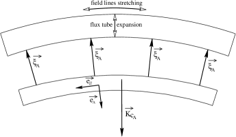
Figure 2: Magnetic flux tube displacement

Generically, pressure-driven instabilities work on a combination of the alfvenic and slow magnetosonic displacements, however, one can devise situations where one or the other dominates. As an example, let us consider the origin of the destabilisation of the Alfvén mode in a static shearless two-dimensional equilibrium with no variation along field lines (it is also possible to devise situations where one primarily destabilizes the magnetosonic mode, but the reasoning is less direct). Let us chose $\@vec{e}_{\!A}$ in the direction of the field line curvature, and consider displacements of a flux tube in the alfvenic direction, and constant along field lines [see fig. (2)]. In this approximation, only Eq. (10) remains, and reduces to

$$\frac{\partial^{2}\xi_{A}}{\partial t^{2}}=V_{A}^{2}\left(2\beta{\mathcal{K}}_{c_{\!A}}{\mathcal{K}}_{\rho_{\!A}}-4\frac{\beta}{1+\beta}{\mathcal{K}}_{c_{\!A}}^{2}\right)\xi_{A}.$$ (17)

Instability follows if the right-hand side member of this equation amplifies the motion, i.e. if

$${\mathcal{K}}_{\rho_{\!A}}>\frac{2}{1+\beta}{\mathcal{K}}_{c_{\!A}}.$$ (18)

This criterion reduces to the well-known criterion of instability with respect to $m=0$ modes (known as the “saussage” mode, which is a pressure-driven mode) in cylindrical systems, (Kadomtsev 1966; see next subsection); it can be more directly established in the following way.

Because the total pressure perturbation cancels, stability with respect to the applied displacement is controlled by the sign of the magnetic tension, which, in this case, reduces to $\delta T_{A}=2\rho_{o}V_{A}^{2}{\delta\!b}_{{{\!\text{\tiny$/\!\!/$}}}}{\mathcal{K}}_{c_{\!A}}$ because the perpendicular perturbation of the magnetic field vanishes for such displacements. In this type of displacement, $\nabla.\@vec{\xi}=\nabla.\@vec{\xi}_{\perp}$. The considered displacement of the flux tube is accompanied by a compression or an expansion (i.e. a change in $\nabla.\@vec{\xi}_{\perp}$), whose sign and magnitude depends on properties of the considered equilibrium, and which can be computed from Eq. (48), combined with Eqs. (2) and (7). This procedure finally yields ${\delta\!b}_{{{\!\text{\tiny$/\!\!/$}}}}=\beta[{\mathcal{K}}_{\rho_{\!A}}-2{\mathcal{K}}_{c_{\!A}}/(1+\beta)]\xi_{A}$, whose sign leads to a destabilizing contribution of the magnetic tension when the criterion (18) is satisfied. This reasoning is typical of an interchange instability, and in fact, the ballooning formalism applies to both interchange and ballooning modes.

2.3 Reduction to cylindrical symmetry

The stability properties of the ballooning system of equation has been been largely studied for cylindrical static equilibria in the context of thermonuclear fusion research. In particular, the well-known Suydam criterion provides a necessary condition for stability of the ballooning modes (see Freidberg 1987, chapter 10 and references therein).

In this paper, we follow a different route by relaxing the eikonal condition $\@vec{k}_{\perp}=\nabla\Phi$. Instead, we Fourier transform the displacement vector in the vertical and azimuthal directions: $\@vec{\xi}=\@vec{\xi}_{o}(\@vec{r})\exp(i\omega t-im\theta-ikz)$, i.e. we consider interchange, rather than ballooning modes. Ballooning and interchange stability analyses in static media based on the form of the energy principle derived by Furth et al. 1965 show that the destabilizing term is $\propto\@vec{\mathcal{K}}_{\rho}.\@vec{\mathcal{K}}_{c}$. For cylindrical configurations, this is maximized by chosing $\@vec{e}_{\!A}$ in the radial direction; this choice also leads to the simplest calculations. Therefore we assume $\@vec{e}_{\!A}=-\@vec{e_{r}}$ from now on (the minus sign is arbitrary, and chosen so that important quantities appearing later are positive). This completely specifies the reference frame (${\@vec{e}}_{{{\!\text{\tiny$/\!\!/$}}}}$, $\@vec{e}_{l}$, $\@vec{e}_{\!A}$) introduced previously. The existence of modes which self-consistently satisfy these constraints in the framework of the ballooning expansion is verified in section 3.

Let us define $\@vec{k}=m\@vec{e}_{\theta}/r+k\@vec{e}_{z}$ and ${k}_{{{\!\text{\tiny$/\!\!/$}}}}=\@vec{k}.\@vec{B}_{o}/B_{o}$. The constraint of quasi-perpendicular propagation implies that ${k}_{{{\!\text{\tiny$/\!\!/$}}}}\ll\@vec{k}.\@vec{e}_{l}$; this is satisfied in particular in the vicinity of magnetic resonances, implicitely defined by $mB_{\theta}/r+kB_{z}=0$ (so that ${k}_{{{\!\text{\tiny$/\!\!/$}}}}=0$ on resonant surfaces), where $B_{\theta}$ and $B_{z}$ are the azimuthal and vertical components of the unperturbed magnetic field. In general, due to magnetic shear, the constraint of quasi-perpendicular propagation implies that our system of equations is only valid within a region of limited radial extent for any given mode. However, we are mostly interested in generic conditions for instability rather than on mode structure; this makes this restriction of little importance, since $\omega$ is constant throughout the radial extent of the mode, and not only in the region of validity of our system of equations, so that conditions over $\omega$ established in this region are nonetheless valid for the whole mode. Furthermore, one can define a resonant $k$ for any $m$ and for an arbitrary magnetic surface, so that our analysis applies to the whole structure. Finally, Goedbloed and Sakanaka (1974) have proved an important theorem which implies that, at fixed $m$ and $k$, if there is a (radially) local unstable mode, there must be a globally unstable one with maximal growth rate for this choice of $m$ and $k$; this theorem applies to static equilibrium configurations, i.e. in our case, to nonrotating cylindrical columns. Its relevance for real jets is unclear, due to velocity shear and rotation, but it nevertheless suggests that local stability results (in radius) might be relevant outside their strict domain of validity.

We conclude from this discussion that although the magnetic shear limits in theory the applicability of our analysis to a finite radial region for each mode, this limitation is of limited practical importance. Note furthermore that we have made no assumption concerning the radial behavior of the modes we consider, besides the limitation imposed by the nearly transverse propagation constraint, which in general should limit both amplitude and phase variations to scales much larger than ${k}_{{{\!\text{\tiny$/\!\!/$}}}}^{-1}$ (however, see the discussion of section 3 for an important exception to this rule).

With our choice of reference frame, and the help of the equilibrium relation Eq. (2), the system of equations derived in the preceding section reduces to

$$\left(\omega^{2}-V_{\rm SM}^{2}{k}_{{{\!\text{\tiny$/\!\!/$}}}}^{2}\right){\xi}_{{{\!\text{\tiny$/\!\!/$}}}}=\\ -i\left(2V_{\rm SM}^{2}\mathcal{K}_{c_{\!A}}{k}_{{{\!\text{\tiny$/\!\!/$}}}}+\frac{\Omega_{o}^{2}r^{2}}{1+\beta}\frac{{k}_{{{\!\text{\tiny$/\!\!/$}}}}}{r}+2\Omega_{o}\omega\rho_{o}\frac{B_{\theta}}{B_{o}}\right)\xi_{A},$$ (19)

$$\left[\omega^{2}-({k}_{{{\!\text{\tiny$/\!\!/$}}}}^{2}+k_{o}^{2}+k_{r}^{2})V_{A}^{2}\right]\xi_{A}=\\ i\left(2V_{\rm SM}^{2}\mathcal{K}_{c_{\!A}}{k}_{{{\!\text{\tiny$/\!\!/$}}}}+\frac{\Omega_{o}^{2}r^{2}}{1+\beta}\frac{{k}_{{{\!\text{\tiny$/\!\!/$}}}}}{r}+2\Omega_{o}\omega\frac{B_{\theta}}{B_{o}}\right){\xi}_{{{\!\text{\tiny$/\!\!/$}}}}.$$ (20)

In these equations,

$$k_{r}^{2} =\frac{\Omega_{o}^{2}r}{(1+\beta)V_{A}^{2}}(\mathcal{K}_{c_{\!A}}+\mathcal{K}_{b_{\!A}}-\mathcal{K}_{\rho_{\!A}})$$

$$=\frac{2{\cal K}_{c_{\!A}}}{1+\beta}\left(\frac{\Omega_{o}^{2}r^{2}}{V_{A}^{2}}\right)\frac{1}{r}\left[1-\left(\frac{(1+\beta){\cal K}_{\rho_{A}}}{2{\cal K}_{c_{A}}}\right)\right]$$

$$-\frac{\Omega_{o}^{2}r^{2}}{(1+\beta)V_{A}^{2}}\frac{1}{r^{2}}\left(\frac{\Omega_{o}^{2}r^{2}}{V_{A}^{2}}\right);$$ (21)

$k_{o}$ is defined in terms of the following auxiliary quantities

$$\frac{h}{2\pi r}=\frac{B_{z}}{B_{\theta}},$$ (22)

$$\mathbf{\Gamma}^{{}^{\!+}}\!\mathbf{\Gamma}^{{}^{\!-}}\!=-\frac{2}{r^{2}}\frac{B_{z}^{2}B_{\theta}^{2}}{B_{o}^{4}}\frac{rh^{\prime}}{h},$$ (23)

and reads

$$k_{o}^{2} =-\mathbf{\Gamma}^{{}^{\!+}}\!\mathbf{\Gamma}^{{}^{\!-}}\!+\frac{2\beta}{1+\beta}(\mathcal{K}_{c_{\!A}}+\mathcal{K}_{b_{\!A}}-\mathcal{K}_{{\rho}_{\!A}})\mathcal{K}_{c_{\!A}}.$$

$$=2{\cal K}_{c_{\!A}}^{2}\left(\frac{B_{z}^{2}}{B_{\theta}^{2}}\right)\left(\frac{d\ln h}{d\ln r}\right)+$$

$$4\frac{\beta{\cal K}_{c_{\!A}}^{2}}{1+\beta}\left[1-\left(\frac{(1+\beta){\cal K}_{\rho_{A}}}{2{\cal K}_{c_{A}}}\right)\right]-\frac{2\beta}{1+\beta}\frac{{\cal K}_{c_{A}}}{r}\left(\frac{\Omega_{o}^{2}r^{2}}{V_{A}^{2}}\right).$$ (24)

In Eq. (20), $V_{A}^{2}(k_{o}^{2}+k_{r}^{2})$ plays the rôle of a generalized Brunt-Väisälä frequency; $k_{r}$ arises from the entrainment inertial force term. The term $\mathbf{\Gamma}^{{}^{\!+}}\!\mathbf{\Gamma}^{{}^{\!-}}\!$ symbolizes the remaining component of the product of $\Gamma$ matrices, and represents the effect of the magnetic shear (note that $rh^{\prime}/h=d\ln h/d\ln r$ is the magnetic shear). The terms on the right hand side of Eqs. (19) and (20) represent the coupling between the two modes due to field line curvature, the entrainment inertial force, and the Coriolis force, respectively. Note that ${\cal K}_{c_{A}}=(B_{\theta}/B_{o})^{2}/r$.

3 Dispersion relation and instability conditions

The complete dispersion relation can easily be obtained from Eqs. (19) and (20). However, we are mostly interested in the ${k}_{{{\!\text{\tiny$/\!\!/$}}}}\rightarrow 0$ limit, for reasons exposed below.

3.1 Nonrotating jets

In order to get some grasp of the meaning of Eqs. (19) and (20), let us first consider non-rotating jets. In this case, the MHD perturbation equations become self-adjoint with our approximations, so that $\omega^{2}$ is real.

Interesting general constraints can be derived from the dispersion relation which reads

$$\omega^{4} -\left[{k}_{{{\!\text{\tiny$/\!\!/$}}}}^{2}(V_{A}^{2}+V_{SM}^{2})+k_{0}^{2}V_{A}^{2}\right]\omega^{2}$$

$$+{k}_{{{\!\text{\tiny$/\!\!/$}}}}^{2}({k}_{{{\!\text{\tiny$/\!\!/$}}}}^{2}-k_{c}^{2})V_{SM}^{2}V_{A}^{2}=0,$$ (25)

where $k_{c}^{2}\equiv\mathbf{\Gamma}^{{}^{\!+}}\!\mathbf{\Gamma}^{{}^{\!-}}\!+2\beta{\cal K}_{c_{\!A}}{\cal K}_{\rho_{\!A}}=4\beta{\cal K}_{c_{\!A}}^{2}/(1+\beta)-k_{o}^{2}$. The roots can readily be extracted from this dispersion relation, but their properties are more directly understood in the following way.

The product of the two roots is positive when ${k}_{{{\!\text{\tiny$/\!\!/$}}}}^{2}>k_{c}^{2}$. One can check that this implies that the sum is also positive, so that both roots are positive. Therefore

$${k}_{{{\!\text{\tiny$/\!\!/$}}}}^{2}<k_{c}^{2}$$ (26)

is a necessary condition of instability for the modes considered here; it is also a sufficient condition, because the root product is negative then, implying that one root is negative. This relation implies in particular $k_{c}^{2}>0$, which, in the absence of magnetic shear, reduces to the necessary condition that the ballooning driving term in the energy principle of Furth et al. (1965) be destabilizing and is identical to (18).

Another condition is obtained by taking the limit ${k}_{{{\!\text{\tiny$/\!\!/$}}}}\rightarrow 0$ in the dispersion relation, which yields $\omega^{2}=0$ and $\omega^{2}=V_{A}^{2}k_{o}^{2}$ as the two roots. This implies that

$$k_{o}^{2}<0$$ (27)

is also sufficient (but not necessary) condition of instability of the modes we consider.

To pinpoint the meaning of the second criterion, it is instructive to examin the behavior of the modes when $|{k}_{{{\!\text{\tiny$/\!\!/$}}}}|\ll|k_{c}|,\ |k_{o}|$ (which can always be achieved by an appropriate choice of $k$ for any particular value of $m$). The first mode has $\omega^{2}\simeq 0$. Then, Eq. (20) yields

$$\xi_{A}\simeq\frac{-2i\beta{\cal K}_{c_{A}}{k}_{{{\!\text{\tiny$/\!\!/$}}}}{\xi}_{{{\!\text{\tiny$/\!\!/$}}}}}{(1+\beta)k_{o}^{2}},$$ (28)

which can be inserted in Eq. (19) to obtain

$$\omega^{2}\simeq-V_{SM}^{2}\frac{k_{c}^{2}{k}_{{{\!\text{\tiny$/\!\!/$}}}}^{2}}{k_{o}^{2}}.$$ (29)

For natural reasons, we refer to the modes which exhibit this behavior in the ${k}_{{{\!\text{\tiny$/\!\!/$}}}}\rightarrow 0$ limit to slow (magnetosonic) modes. From the general solution to the dispersion relation, the maximum value of $\omega^{2}$ for this mode is obtained for ${k}_{{{\!\text{\tiny$/\!\!/$}}}}^{2}\sim k_{c}^{2}$, which provides us with an estimate of their maximum growth rate, once inserted in (29). The second mode has

$$\omega^{2}\simeq V_{A}^{2}k_{o}^{2}.$$ (30)

Then Eq. (19) implies

$${\xi}_{{{\!\text{\tiny$/\!\!/$}}}}\simeq\frac{-2i\beta{\cal K}_{c_{A}}{k}_{{{\!\text{\tiny$/\!\!/$}}}}\xi_{A}}{(1+\beta)k_{o}^{2}}.$$ (31)

We refer to modes which exhibit this behavior in the ${k}_{{{\!\text{\tiny$/\!\!/$}}}}\rightarrow 0$ limit as to Alfvén modes. The maximum growth rate for these modes is reached for ${k}_{{{\!\text{\tiny$/\!\!/$}}}}=0$.

With these definitions, the slow modes are unstable and the Alfvén ones stable when $k_{c}^{2}>{k}_{{{\!\text{\tiny$/\!\!/$}}}}^{2}$ and $k_{0}^{2}>0$; the situation is reversed when $k_{c}^{2}>{k}_{{{\!\text{\tiny$/\!\!/$}}}}^{2}$ and $k_{0}^{2}<0$. Both modes are stabilized by the usual contribution to the magnetic tension when ${k}_{{{\!\text{\tiny$/\!\!/$}}}}^{2}>k_{c}^{2}$.

Note that when the magnetic shear is important, ${\xi}_{{{\!\text{\tiny$/\!\!/$}}}}$ for the Alfvén mode, and $\xi_{A}$ for the slow mode, undergo fast radial variations. One can check that fast radial variations of ${\xi}_{{{\!\text{\tiny$/\!\!/$}}}}$ are not inconsistent with our procedure, which is not true for $\xi_{A}$. Therefore, when this occurs, one must discard the slow mode, which is not a self-consistent solution of our system of equations.

3.2 Jets with vanishing current density on the axis

There are situations in which one expects that $B_{\theta}$ increases with $r$ faster than $r$ in jet inner regions (in which case the current density vanishes on the axis). Indeed, for jets which are launched from an accretion disk, $u_{z}B_{\theta}/B_{z}=r(\Omega-\Omega_{\star})$ where $\Omega$ and $\Omega_{\star}$ are the matter and field rotation respectively, $u_{z}$ is the jet velocity along the jet axis (Pelletier and Pudritz, 1992). In these regions, one usually expects $u_{z}\neq 0$, while $\Omega,\Omega_{\star}\rightarrow 0$ when $r\rightarrow 0$. Furthermore, polarisation observations indicate that the magnetic field is predominantly aligned with the jet axis in jet cores, at least for quasar jets (see Gabuzda, 1997, and references therein). It is therefore reasonable to expect that $|B_{\theta}|<$ or $\ll|B_{z}|$ over a sizeable fraction of the inner region of these jets. In these regions, $k_{0}^{2}<0$ is automatically satisfied because the shear term dominates (as rotation is unimportant there) and is negative [see Eq. (24)], so that the inner regions of these jets are generically unstable. Note that our neglect of the velocity shear in the derivation of our equations has no impact on this conclusion, because both rotation and velocity shear terms are expected to be negligible in the considered jet regions. Obviously, $|B_{z}|$ must exceed $|B_{\theta}|$ over a sizeable fraction of the jet interior for the instability to have noticeable effects and growth rates.

The destabilizing action of the magnetic shear just pointed out is the most important finding of this paper. It can be given a heuristic explanation in the following way. Regions with a destabilizing contribution of the magnetic shear are regions in which the shear contributes to an extra-increase of the Alfvénic component of the equilibrium tension when one moves outwards. Applying a purely radial displacement to a magnetic flux tube (i.e., considering an Alfvénic mode with ${k}_{{{\!\text{\tiny$/\!\!/$}}}}=0$) produces a variation of the Alfvénic component of the magnetic tension which does not include this extra piece due to the magnetic shear; therefore, the variation in the magnetic tension produces a restoring force on the displaced flux tube which is smaller than the restoring force on the equilibrium flux tube at the same location, and instability follows.

Note also that we must discard the magnetosonic mode, which is no longer a valid solution of our equations due to the fast amplitude gradients of $\xi_{A}$ induced by the shear, as explained in the preceding section.

3.3 Nonrotating jets dominated by the toroidal field

In magnetically confined jets, one usually assumes $|B_{\theta}|\gg|B_{z}|$ in the confining region (“Z-pinch” configurations). This follows in particular when jets are launched from accretion disks, because they must open considerably before the critical surfaces are crossed, and the magnetic collimation becomes important. This boosts the ratio $|B_{\theta}/B_{z}|$ first because the poloidal flux is conserved within magnetic surfaces, second because the toroidal field is considerably stretched in the process, while this ratio is expected to be of order unity on the disk “surface” (Ferreira 1997; Casse and Ferreira 2000). In this case, ${k}_{{{\!\text{\tiny$/\!\!/$}}}}\simeq m/r+kB_{z}/|B_{\theta}|$ and $k_{\perp}\simeq k$. Furthermore ${k}_{{{\!\text{\tiny$/\!\!/$}}}}$ depends on the radial location; Eq. (31) shows that ${\xi}_{{{\!\text{\tiny$/\!\!/$}}}}$ contain no large amplitude variations [as implicitly assumed in the derivation of Eqs. (19) and (20)] provided that $|krB_{z}/B_{\theta}|\lesssim 1$ and $|m|\lesssim 1$ (note however that fast amplitude variations of $\xi_{A}$ do not invalidate the derivation of these equations). Then, the condition of quasi-perpendicular propagation is satisfied for $|kr|\gg 1$ (as $m$ is a small integer).

When these conditions of consistency of the slow mode with our approximations hold, one can eliminate all gradients in terms of logarithmic gradients of $B_{\theta}$ (the gradient of $B_{z}$ vanishes or is negligible). This allows us to reexpress $k_{o}$ as

$$k_{o}^{2}=4\frac{\beta{\cal K}_{c_{\!A}}^{2}}{1+\beta}\left[1-\left(\frac{1+\beta}{2\beta}\right)\left(r\frac{d\ln rB_{\theta}}{dr}\right)\right].$$ (32)

The shear term has disappeared because it is negligible for $|B_{\theta}|\gg|B_{z}|$; the first term in brackets represents the stabilizing action of the plasma compression (it arises from the divergence of the displacement), while the other term represents the action of pressure gradients, either stabilizing or destabilizing. The expression for $k_{c}^{2}$ is very similar, and obtained by changing the sign and removing the compression term.

The limit $|B_{\theta}|\gg|B_{z}|$, completed with $|kr|\gg 1$ and $|krB_{\theta}/B_{z}|\lesssim 1$ allows us to connect with previously derived results on pressure-driven instabilities. In this case, one has ${k}_{{{\!\text{\tiny$/\!\!/$}}}}={\rm sgn}(B_{\theta})m/r+kB_{z}/|B_{\theta}|$, ${\cal K}_{c_{A}}=1/r$, and the criterion (26) becomes, with the help of Eq. (32):

$$\frac{d\ln{|B_{\theta}|}}{d\ln r}>\frac{1}{2}\left(m+kr\frac{B_{z}}{B_{\theta}}\right)^{2}-1,$$ (33)

which has been derived for $m=1$, $k=0$ modes with $\nabla.\@vec{\xi}=0$ by Kadomtsev (1966), and for an arbitrary mode by Begelman (1998).

The condition (27) which identifies the Alfvén branch as the unstable one reads in the same limit:

$$\frac{d\ln|B_{\theta}|}{d\ln r}>\frac{\beta-1}{\beta+1},$$ (34)

a condition also obtained by Kadomtsev (1966) and Begelman (1998) for the $m=0$ “saussage” mode (remember that our definition of $\beta$ differs from the standard one by a factor $\gamma/2$).

We point out again that (33) [or equivalently (26)] is a necessary and sufficient condition for having unstable modes, but (34) is a condition for the Alfvén branch to be unstable; these conditions do not assume any particular value of $m$ and do not rely on an incompressibility assumption. These points are often overlooked in the literature. Note however that for smooth profiles, $k_{c}^{2}\gtrsim 1/r^{2}$, so that (33) limits $m$ to small values, independently of the limit obtained from the consistency requirement of the slow mode. It is well-known that condition (34) is easy to meet in practice; in particular, it is always satisfied for a Lorentzian (or Bennett) profile. ) We conclude with Begelman (1998) that the configurations usually considered for magnetically confined jets are generically unstable in the absence of rotation. Indeed, the condition for instability Eq. (26) is always satisfied for $m=0$, and probably $m=1$ as well in jet inner regions, because $|B_{\theta}|$ must increase from zero on the axis to values $|B_{\theta}|\gg|B_{z}|$ in inner regions; in general it decreases too fast in most jet models when moving towards the jet radial boundary for outer regions to be unstable. Furthermore Eq. (34) implies that the Alfvén mode is very likely to be the unstable mode.

3.4 Rotating jets dominated by the toroidal field

Rotation, in particular the Coriolis force, introduces an extra-coupling between the Alfvénic and magnetosonic part of the displacements, which is not vanishing in the ${k}_{{{\!\text{\tiny$/\!\!/$}}}}\rightarrow 0$ limit. Nevertheless, we stick with our distinction between Alfvén and slow magnetosonic modes, although it is less meaningful in this context.

It is useful to characterize the jet rotation by introducing $\chi\equiv\Omega_{o}^{2}r^{2}/V_{A}^{2}$. The equilibrium condition Eq. (2) implies that $\chi$, like $\beta$, is of order unity at most. More specifically, one has (Pelletier and Pudritz 1992)

$$\chi=\frac{1}{M^{2}}\frac{(1-M^{2}r_{A}^{2}/r^{2})^{2}}{(1-r_{A}^{2}/r^{2})^{2}},$$ (35)

where $M$ is the poloidal Mach number and $r_{A}$ is the Alfvén radius. In strong jets, one has $M^{2}r_{A}^{2}/r^{2}\sim 1$ whereas $r$ is always larger (possibly much larger) than $r_{A}$, which, as stated, implies that $\chi$ is of order unity at most. We assume $\chi\lesssim 1$, which maximizes the influence of rotation on the dynamics.

The influence of the jet rotation is again analyzed by deriving the dispersion relation, which reads:

$$\omega^{4}- \left[{k}_{{{\!\text{\tiny$/\!\!/$}}}}^{2}(V_{A}^{2}+V_{SM}^{2})+(k_{0}^{2}+k_{r}^{2})V_{A}^{2}+4\Omega_{o}^{2}(B_{\theta}^{2}/B_{o}^{2})\right]\omega^{2}$$

$$-4\Omega_{o}(B_{\theta}/B_{o}){k}_{{{\!\text{\tiny$/\!\!/$}}}}V_{SM}^{2}\left(2{\cal K}_{c_{A}}+\frac{\chi}{\beta r}\right)\omega$$

$$+{k}_{{{\!\text{\tiny$/\!\!/$}}}}^{2}\bigg{[}{k}_{{{\!\text{\tiny$/\!\!/$}}}}^{2}-k_{c}^{2}+k_{r}^{2}$$

$$-\frac{\chi}{(1+\beta)}\left(2{\cal K}_{c_{A}}+\frac{\chi}{\beta r}\right)\bigg{]}V_{SM}^{2}V_{A}^{2}=0,$$ (36)

where $k_{o}^{2}$ and $k_{r}^{2}$ are given in Eqs. (24) and (21).

In the limit ${k}_{{{\!\text{\tiny$/\!\!/$}}}}=0$, this equation has two roots, the magnetosonic branch (whose degeneracy is broken by rotation) $\omega^{2}=0$, and the Alfvénic branch

$$\omega^{2}=V_{A}^{2}\left(k_{o}^{2}+k_{r}^{2}\right)+4\Omega_{o}^{2}\left(\frac{B_{\theta}^{2}}{B_{o}^{2}}\right).$$ (37)

The last term in this relation is due to the Coriolis force and is always stabilizing. This is a natural consequence of the form of this force, $\@vec{\Omega}_{o}\times\@vec{\xi}$, which gives rise to coupled oscillations between the components of the displacement vector. The factor $B_{\theta}/B_{o}$ arises because of the inclination of the magnetic vector $\@vec{B}_{o}$ with respect to the rotation axis.

The discussion of the stability properties in the absence of rotation implies that stabilization by rotation will only occur when $\chi\sim 1$. To quantify somewhat this statement, let us rewrite $k_{o}^{2}$ and $k_{r}^{2}$ as

$$k_{o}^{2}=\frac{1}{r^{2}}\frac{4\beta}{1+\beta}\left[1-\frac{1+\beta}{2\beta}\frac{d\ln r|B_{\theta}|}{d\ln r}\right]+\frac{2\chi}{r^{2}(1+\beta)},$$ (38)

$$k_{r}^{2}=\frac{2\chi}{r^{2}(1+\beta)}\left[1-\frac{1+\beta}{2\beta}\frac{d\ln r|B_{\theta}|}{d\ln r}\right]+\frac{\chi^{2}}{r^{2}\beta(1+\beta)}.$$ (39)

It is apparent that the contribution of the jet rotation to $k_{o}^{2}$ is always stabilizing. Furthermore, the pressure contributions to $k_{0}^{2}$ and $k_{r}^{2}$ are destabilizing when condition (34) is satisfied. The arguments of the previous subsection make this very likely to happen in the inner region of jets. A condition on the critical gradient of $B_{\theta}$ can easily be extracted, but it is not very informative. Instead, limits of instability can be obtained in the following way. We assume that $d\ln|B_{\theta}|/d\ln r\simeq 1$; this applies in jet inner regions when the behavior of the magnetic shear is not controlled by rotation, as in the previous section. The dispersion relation (37) implies then that $\beta\lesssim 1/4$ for $\chi\simeq 1$ or reversely $\chi\lesssim 1/2$ for $\beta\simeq 1$ constitute sufficient conditions of instability. This implies that it is very difficult in practice to stabilize the Alfvén mode by rotation, especially that jets possessing an important cylindrical asymptotic limit have $\chi\ll 1$ from Eq. (35), as such jets have $M\gg 1$.

Note that stability occurs for high $\beta$, whereas in the fusion context, the reverse is true. This follows because destabilisation is provided by the rotation entrainment force rather than pressure forces.

The stability properties of the slow mode can be discussed in the ${k}_{{{\!\text{\tiny$/\!\!/$}}}}\rightarrow 0$ limit. Assuming that the frequency of magnetosonic modes $\omega\propto{k}_{{{\!\text{\tiny$/\!\!/$}}}}$ for small enough ${k}_{{{\!\text{\tiny$/\!\!/$}}}}$, as implied by the dispersion relation, and keeping only the leading order term in ${k}_{{{\!\text{\tiny$/\!\!/$}}}}$ yields a reduced dispersion relation:

$$A\omega^{2}+B\omega+C=0,$$ (40)

where

$$A =\left[(k_{0}^{2}+k_{r}^{2})V_{A}^{2}+4\Omega_{o}^{2}(B_{\theta}^{2}/B_{o}^{2})\right],$$

$$B =4\Omega_{o}(B_{\theta}/B_{o}){k}_{{{\!\text{\tiny$/\!\!/$}}}}V_{SM}^{2}\left(2{\cal K}_{c_{A}}+\frac{\chi}{\beta r}\right)$$

$$C ={k}_{{{\!\text{\tiny$/\!\!/$}}}}^{2}\left(-k_{c}^{2}+k_{r}^{2}-\frac{\chi}{r(1+\beta)}\left(2{\cal K}_{c_{A}}+\frac{\chi}{\beta r}\right)\right)V_{SM}^{2}V_{A}^{2}.$$ (41)

Because of the term $\propto\omega$ in this reduced dispersion relation, overstability rather than instability occurs when the discriminant $\Delta\equiv B^{2}-4AC<0$. It turns out that for $\chi\simeq 1$ and $d\ln B_{\theta}/d\ln r\simeq 1$, $\Delta>0$ whatever the value of $\beta$, implying that the slow mode is stabilized by rotation in the small ${k}_{{{\!\text{\tiny$/\!\!/$}}}}$ limit.

This suggests that the slow mode is more easily stabilized than the Alfvénic one. In any case, our result on the Alfvén mode is sufficient to conclude that jets with a dominant toroidal field are difficult to stabilize by rotation.

4 Discussion

In this paper, we have focused on the stability of rotating MHD jets with respect to inhomogeneities connected to pressure gradients and magnetic shear, in the framework of the ballooning ordering. The most remarkable finding of our analysis is the possible destabilizing influence of the magnetic shear pointed out in section 3. Indeed, the shear appears quadratically in Suydam’s well-known criterion, which applies to the stability of cylindrical columns, whereas the stability criterion of the preceding section is linear in magnetic shear. We point out that, had we not relaxed the eikonal condition in section 2, we would have recovered Suydam’s criterion (see Freidberg 1987, Chapter 10). This unexpected behavior of the magnetic shear implies that the inner regions of jets launched from accretion disks are generically unstable, as argued in section 3.

We have also recovered that for jet models dominated by a toroidal magnetic field, jet interiors are likely to be subject to this type of instability, a result already pointed out by Begelman (1998). Furthermore, we find that rotation has little influence on this conclusion; rotation can only stabilize jets when it is close to the limit allowed by the radial equilibrium condition, and for values of $\beta$ close to the same limit.

Our results on pressure-driven instabilities agree with those found in the literature, most notably Begelman (1998) and Ferrière et al. (1999), once appropriate limits are taken. Begelman’s study is restricted to $B_{\theta}/B_{z}\gg 1$, which removes the effect of the magnetic shear from the analysis. Ferrière et. al. (1999) do not rely on the ballooning expansion, keep the full six-dimensional dispersion relation, and discuss in detail the effects of rotation and gravity, besides gas pressure and field curvarture. They give a detailed and interesting synthesis of gravitational and centrifugal instabilities in magnetospheric studies. However, to achieve such a generality, they rely on a particular coordinate representation of the magnetic field, which is well-adapted to planetary magnetospheres, but forbids also the presence of magnetic shear.

Jet models which are not dominated by the toroidal magnetic field have been proposed in the literature. One example is the force-free jet model of Appl and Camenzind, 1992, which has $B_{\theta}\sim B_{z}$, and belongs to a class of configurations known as “reversed field pinch” in the fusion research context. These configurations are known to be stable with respect to pressure-driven instabilities for moderately low values of $\beta$ (and, more generally, to possess good stability properties). This apparently conflicts with our results on destabilization by the shear. However, we point out that destabilization occurs because $B_{\theta}$ varies faster than $r$ in the jet inner region. This variation is induced by the behavior of the jet matter and field rotation, a feature which is absent from fusion control devices.

In this analysis as in all others we are aware of, we have assumed that the jet equilibrium structure is invariant along the jet axis. This need not be the case, as examplified in various self-similar solutions (Sauty and Tsinganos, 1994; Contopoulos and Lovelace, 1994), and more recenly in a complete analytic solution displaying a more complex magnetic field structure (Bogoyalenskij, 2000). The relevance of the available stability analyses to such configurations is unclear; furthermore, these configurations are possibly unstable with respect to appropriately chosen ballooning modes. In any case, this question should be addressed before firm conclusions can be drawn.

We have not tried to derive precise growth rates, as these depend on the radial structure of the most unstable modes, the determination of which is outside the scope of the approximation scheme we have adopted. However, order of magnitude considerations show that these instabilities should develop within a few dynamical time-scale ($\sim aV_{A}^{-1}$ where $a$ is the characteristic radial size of the considered region).

Let us also return to the question of overstability, which was briefly alluded to in section 2 and 3. Our dispersion relation shows that $\omega^{2}$ is real for alfvenic modes in the ${k}_{{{\!\text{\tiny$/\!\!/$}}}}=0$ limit, implying that $\omega$ is real when $\omega^{2}>0$. This property remains true when $\omega({k}_{{{\!\text{\tiny$/\!\!/$}}}})$ is computed as a series in ${k}_{{{\!\text{\tiny$/\!\!/$}}}}$, to all orders in this series if it is true to lowest order (this can be shown by induction from the full dispersion relation, because it involves only real terms). Therefore the stability property of the Alfvén mode is obtained in the ${k}_{{{\!\text{\tiny$/\!\!/$}}}}=0$ limit. In the same way, the dispersion relation of Ferrière et. al. (1999) [their Eq. (27)] implies that the fast magnetosonic mode is stable in the absence of magnetic shear in the perpendicular WKB approximation. This suggests that the fast mode is probably not destabilized in the asymptotic limit examined in this paper.

We point out again that, in spite of their partly local nature, pressure-driven instabilities, and magnetic shear-driven ones as well, are likely to produce large-scale disruptions of MHD jets. How real jets survive these instabilities as well as Kelvin-Helmholtz and current-driven instabilities is a still open and pressing problem, especially that 3D instabilities seem more vigorous than there 2D counterparts (see, e.g., Bodo et al., 1998). However, progress on this topic has recently been accomplished. For the Kelvin-Helmholtz instability, recent 3D simulations have shown that for initial magnetic Reynolds numbers smaller than $\sim 50$, the shear layer broadens, the turbulence level decreases and the flow becomes quasi-laminar and stable in the end (Ryu et al., 2000); as jets are not expected to be drastically out of equipartition, and as the Lorentz force provides the origin of their acceleration, this probably ensures their stability against a possible disruption by the Kelvin-Helmholtz instability. Also, the kink instability seems to lead to helicoidal equilibria with a redistribution of the current density rather than to disruption (Lery et al., 2000). Finally, it has recently been recognized in the fusion literature that pressure-driven instabilities can be stabilized by large equilibrium gradients, a somewhat counterintuitive result (Terry, 2000).

One of the interesting questions raised by this work concerns the possible link between the type of instabilities we consider and the particle acceleration mechanism which is responsible for the high energy emission seen in AGN jet interiors. For example, in the context of the two-flow model, most of the high energy emission comes from a highly relativistic pair plasma occupying the inner region of a slower jet which contains most of the mass and provides most of the energy. This model relies on energy injection to the pair plasma from the bulk of the jet through turbulence (Renaud and Henri, 1998); note also that the existence of a pair plasma in AGN jets has recently received an interesting observational support (Wardle, et. al., 1998; Hirotani et. al., 1998). In such a picture of the high energy emission, the required turbulence would most likely be provided by MHD instabilities in the nonlinear regime, as other sources look unpromising. Indeed, a purely hydrodynamical origin in regions of increasing angular velocity with radius, as advocated by Richard and Zahn (1999) is not found in numerical simulations (Balbus et al., 1996), and happens in laboratory Couette experiments (performed in general with narrow gap widths between the inner and outer cylinder) only when the outer cylinder completely dominates the rotation (Coles, 1965), a situation which has little connection with disks and jets; furthermore, the magneto-rotational instability (Balbus and Hawley, 1991) does not work in this regime, and the velocity shear is ineffective in driving the Kelvin-Helmholtz instability in the subalfvenic portion of the jet in jet interiors.

To conclude, let us finally point out that pressure-driven modes are also known to be avalanche-like instabilities, due to the existence of a critical gradient, and this feature raises important question concerning the action of this instability on jet profiles, as well as their role in jet variability.

Appendix A MHD perturbation equations and the ballooning approximation

Let us first recall some properties of wave propagation in homogeneous media. In the reference frame introduced in section 2.2, the momentum equation yields the following three component equations

$$\left(\omega^{2}-C_{S}^{2}\,{k}_{{{\!\text{\tiny$/\!\!/$}}}}^{2}\right)\,{\xi}_{{{\!\text{\tiny$/\!\!/$}}}}=C_{S}^{2}\,{k}_{{{\!\text{\tiny$/\!\!/$}}}}\,k_{\perp}\,\xi_{l},$$ (42)

$$\left(\omega^{2}-C_{S}^{2}\,k_{\perp}^{2}-V_{A}^{2}\,k^{2}\right)\,\xi_{l}=C_{S}^{2}\,{k}_{{{\!\text{\tiny$/\!\!/$}}}}\,k_{\perp}\,{\xi}_{{{\!\text{\tiny$/\!\!/$}}}},$$ (43)

$$\left(\omega^{2}-V_{A}^{2}\,{k}_{{{\!\text{\tiny$/\!\!/$}}}}^{2}\right)\,\xi_{A}=0,$$ (44)

while the total pressure perturbation becomes

$$\delta\!P_{\ast}=-i{\rho}_{\!o}\left[(C_{S}^{2}+V_{A}^{2})\,k_{\perp}\xi_{l}+C_{S}^{2}\,{k}_{{{\!\text{\tiny$/\!\!/$}}}}{\xi}_{{{\!\text{\tiny$/\!\!/$}}}}\right].$$ (45)

Eq. (44) gives the dispersion relation of Alfvén waves, $\omega_{A}^{2}=V_{A}^{2}{k}_{{{\!\text{\tiny$/\!\!/$}}}}^{2}$, which decouple from the two magnetosonic modes described by the remaining two equations. In the approximation of interest here ($\epsilon={k}_{{{\!\text{\tiny$/\!\!/$}}}}/k_{\perp}\ll 1$, i.e. nearly perpendicular propagation), these two equations imply $\omega_{S}^{2}\simeq C_{S}^{2}V_{A}^{2}/(C_{S}^{2}+V_{A}^{2}){k}_{{{\!\text{\tiny$/\!\!/$}}}}^{2}$ and $\xi_{l}\sim O(\epsilon{\xi}_{{{\!\text{\tiny$/\!\!/$}}}})$ for the slow magnetosonic wave, while $\omega_{F}^{2}\simeq(C_{S}^{2}+V_{A}^{2}){k}_{{{\!\text{\tiny$/\!\!/$}}}}^{2}$ and ${\xi}_{{{\!\text{\tiny$/\!\!/$}}}}\sim O(\epsilon\xi_{l})$ for the fast magnetosonic one.

Furthermore, the $\xi_{l}$ momentum component Eq. (43) combined with Eq. (44) implies that $\delta\!P_{\ast}=0$ to leading order in $\epsilon$.

Let us now turn to inhomogeneous and non-static media. The ordering assumed in Eqs. (8) and (9) implies that the longitudinal component of the momentum equation [Eq. (1)] reduces to

$$\delta\!P_{\ast}=\delta\!P+\frac{{\@vec{B}}_{\!o}\!\cdot\!\delta\!\@vec{B}}{\mu}=0.,$$ (46)

to leading order in $\epsilon$. In establishing this result, the unperturbed momentum equation [Eq. (2)] has been used to show that $\Omega_{o}\sim\omega$ at most. The total pressure perturbation cancels because in the quasi-perpendicular propagation assumed here, slow and alfvenic perturbations behave quasistatically in the fast direction, and because fast perturbations are only compressional in the fast direction in homogeneous media, implying that inhomogeneous corrections are negligible in our WKB-like approximations. To derive the remaining two momentum component equations, we need to evaluate the tension perturbation in terms of the displacement $\@vec{\xi}$ [the entrainment inertial term follows immediately from the perturbed density Eq. (5)]

$$\delta\!\@vec{T}=\frac{{\@vec{B}}_{\!o}\!\cdot\!\nabla\delta\!\@vec{B}}{\mu}+\frac{\delta\!\@vec{B}\!\cdot\!\nabla{\@vec{B}}_{\!o}}{\mu}.$$ (47)

The magnetic field perturbation $\delta\!\@vec{b}=\delta\!\@vec{B}/{B}_{\!o}$ [cf Eq. (6)] along and perpendicular to the unperturbed magnetic field read

$${\delta\!b}_{{{\!\text{\tiny$/\!\!/$}}}}=-\nabla\!\cdot\!\@vec{\xi}_{\perp}-\left(\@vec{\mathcal{K}}_{b_{\!\perp}}+\@vec{\mathcal{K}}_{c}\right)\!\cdot\!\@vec{\xi}_{\perp},$$ (48)

$$\delta\!\@vec{b}_{\perp} =\mathbf{\Gamma}^{{}^{\!-}}\!\!\cdot\!\@vec{\xi}_{\!\perp}+\frac{\partial\xi_{l}}{\partial s}\,\@vec{e}_{l}+\frac{\partial\xi_{A}}{\partial s}\,\@vec{e}_{\!A}+\left(\@vec{\xi}\!\cdot\!\@vec{\mathcal{K}}_{c}\right){\@vec{e}}_{{{\!\text{\tiny$/\!\!/$}}}}$$

$$=\begin{pmatrix}\displaystyle\mathbf{\Gamma}^{{}^{\!-}}\!_{{}_{\!\!\!\!\mathbf{ll}}}\,\xi_{l}+\mathbf{\Gamma}^{{}^{\!-}}\!_{{}_{\!\!\!\!\mathbf{lA}}}\,\xi_{A}+\frac{\partial\xi_{l}}{\partial s}\\[11.38092pt] \displaystyle\mathbf{\Gamma}^{{}^{\!-}}\!_{{}_{\!\!\!\!\mathbf{Al}}}\,\xi_{l}+\mathbf{\Gamma}^{{}^{\!-}}\!_{{}_{\!\!\!\!\mathbf{AA}}}\,\xi_{A}+\frac{\partial\xi_{A}}{\partial s}\end{pmatrix}\ ,$$ (49)

where the matrices $\mathbf{\Gamma}^{{}^{\!+}}\!$ and $\mathbf{\Gamma}^{{}^{\!-}}\!$ are defined in Eq. (16), $\partial/\partial s\equiv{\@vec{e}}_{{{\!\text{\tiny$/\!\!/$}}}}.\nabla$, and the various $\cal K$s are defined right before Eq. (2).

In Eq. (48), the first term represents the variation of the field in its original direction due to the conservation of magnetic flux in transverse compression of the plasma; the second term represents the contribution of field advection, the last one the contribution of field line stretching.

With these results, the perpendicular component of the tension perturbation reads

$$\delta\!T_{\{l,A\}}={\rho}_{\!o}\,V_{A}^{2}\left(\frac{\partial}{\partial s}\delta\!b_{\{l,A\}}+\mathcal{K}_{b_{/\!\!/}}\delta\!b_{\{l,A\}}\right.\\[4.79993pt] \left.+\,\@vec{e}_{\{l,A\}}\!\cdot\!\mathbf{\Gamma}^{{}^{\!+}}\!\!\cdot\!\delta\!\@vec{b}_{\perp}+2\,\delta\!{b}_{{{\!\text{\tiny$/\!\!/$}}}}\,\mathcal{K}_{c_{\{l,A\}}}\right),$$ (50)

while the parallel tension perturbation is given by

$$\delta\!{T}_{{{\!\text{\tiny$/\!\!/$}}}}={\rho}_{\!o}\,V_{A}^{2}\,\left[\delta\!\@vec{b}_{\perp}\!\cdot\!\left(\@vec{\mathcal{K}}_{b_{\!\perp}}-\@vec{\mathcal{K}}_{c}\right)+\frac{\partial{\delta\!b}_{{{\!\text{\tiny$/\!\!/$}}}}}{\partial s}+2\mathcal{K}_{b_{/\!\!/}}{\delta\!b}_{{{\!\text{\tiny$/\!\!/$}}}}\right].$$ (51)

These equations for the perturbed magnetic field and magnetic tension are exact (the ordering has not been used in their derivation). Furthermore, by noting that

$$\nabla\!\cdot\!\@vec{\xi}_{\perp}=\frac{\partial{\xi}_{{{\!\text{\tiny$/\!\!/$}}}}}{\partial s}-{\xi}_{{{\!\text{\tiny$/\!\!/$}}}}\,\mathcal{K}_{b_{/\!\!/}}-\nabla\!\cdot\!\@vec{\xi},$$ (52)

it appears that derivatives of the displacement in the magnetic force term enter only through derivative along the field line and $\nabla.\@vec{\xi}$; the same crucial feature holds for the entrainment inertial force term, while the derivatives of the displacement do not enter the expression of the Coriolis force term. With the help of the cancellation of the total pressure perturbation Eq. (46), one can express $\nabla.\@vec{\xi}$ in terms of $\@vec{\xi}$ and of the derivatives of the components of $\@vec{\xi}$ in the field line direction. This yields

$$\nabla\!\cdot\!\@vec{\xi}= -\frac{1}{1+\beta}\left[\left(\beta\mathcal{K}_{\rho_{\!A}}+\mathcal{K}_{b_{\!A}}+\mathcal{K}_{b_{\!A}}\right)\xi_{A}\right.$$ (53)

$$+\beta\left(\frac{\partial}{\partial s}-\mathcal{K}_{b_{/\!\!/}}+\mathcal{K}_{\rho_{/\!\!/}}\right){\xi}_{{{\!\text{\tiny$/\!\!/$}}}}$$

$$\left.-\left(1+\beta\right)\left(\mathcal{K}_{b_{\!A}}+\mathcal{K}_{c_{\!A}}\right)\xi_{a}\right]$$

This reduces the problem to the set of ordinary differential equations for ${\xi}_{{{\!\text{\tiny$/\!\!/$}}}}$ and $\xi_{A}$ given in Eqs. (10) and (11).

References

- (1) Appl, S., Camenzind, M., 1992, A& A 256, 354.
- (2) Appl, S., A& A 314, 995.
- (3) Balbus, S.A., Hawley, J.F., Stone, J.M., 1996, ApJ, 467, 76.
- (4) Bateman, G., 1978, MHD instabilities, MIT Press, Cambridge Mass.
- (5) Belgelman, M.C., 1998, ApJ 493, 291.
- (6) Benford, G. 1978, MNRAS 183, 29.
- (7) Birkinshaw, M., 1991, in: Beams and Jets in Astrophysics, ed. P.A. Hugues, Cambridge Univ. Press, Cambridge.
- (8) Blandford, R.D., Payne, D.G., 1982, MNRAS 199, 883.
- (9) Bodo, G., Rossi, Massaglia, S., Ferrari, A., Malagoli, A., Rosner, R., 1998, A&A, 333, 1117.
- (10) Casse, F. Ferreira, J., 2000, A& A, 353, 1115.
- (11) Chan, K.L., Henriksen, R.N., 1980, ApJ, @41, 534.
- (12) Coppi, B., Filreis, J., Pegoraro, F., 1979, Ann. Phys. N.Y. 121, 1.
- (13) Contopoulos, J., Lovelace, R.V.E., 1994, ApJ, 429, 139.
- (14) Coles, D., 1965, J. Fluid Mech., 21, 385.
- (15) Dewar, R.L., Glasser, A.H., 1983, Phys. Fluids 26, 3038.
- (16) Ferrière, K.M., Zimmer, C., Blanc, M., 1999, JGR 104, 17335.
- (17) Ferreira, J., 1997, A& A, 319, 340.
- (18) Freidberg, J.P., 1987, Ideal Magnetohydrodynamics, Plenum Press, New York.
- (19) Furth, H.P., Killeen, J., Rosenbluth, M.N., Coppi, B., 1965, in: Plasma Physics and Controlled Nuclear Fusion Research, IAEA, Vienna, Vol. 1, p. 103.
- (20) Gabuzda, D.C., 1997, in: Relativistic Jets in AGNs, eds. M Ostrowski, M. Sikora, G. Madejski, M. Begelman, Cracow.
- (21) Kadomtsev, B.B., 1966, in: Reviews of Plasma Physics, ed. M.A. Leontovitch, Consultants Bureau, New York, Vol. II.
- (22) Hardee, P.E., Stone, J.M., 1997, ApJ 483, 121.
- (23) Hood, A.W., 1986, Sol. Phys. 103, 329.
- (24) Hirotani, K., Igushi, S., Kimura, M., Wajima, K., PASJ, 51, 263.
- (25) Lery, T., Baty, H., Appl, S., 2000, A&A, 355, 1201.
- (26) Newcomb, W.A., 1961, Phys. Fluids 4, 391.
- (27) Pelletier, G., Pudritz, R.E., 1992, ApJ 394, 117.
- (28) Renaud, N., Henri, G., 1998, MNRAS, 300, 1047.
- (29) Richard, D., Zahn, J.-P., 1999, A &A, 347, 734.
- (30) Ryu, D., Jones, T.W., Frank, A., astro-ph/0008084.
- (31) Sauty, C, Tsinganos, K., A &A, 287, 893.
- (32) Stone, J.M., Xu, J., Hardee, P.E., 1997, ApJ 483, 136.
- (33) Terry, P.W., 2000, Rev. Modern Phys., 72, 109.
- (34) Wardle, J.F.C., Homan, D.C., Ojha, R., Roberts, D.H., 1998, Nature, 395, 457.