Optical photometry of the UCM Lists I and II

Abstract

We present Johnson $B$ surface photometry for the UCM Survey galaxies. One-dimensional bulge-disk decomposition is attempted, discussing on fitting functions and computational procedures. The results from this decomposition, jointly with concentration indices and an asymmetry coefficient, are employed to study the morphological properties of these galaxies. We also compare our results with the previous morphological classification established using Gunn $r$ imaging data and with other samples of galaxies. No major statistical differences in morphology are found between red and blue data, although some characteristics such as size and luminosity concentration vary. We find a correlation between luminosity and size. Several parameters are used to segregate the objects according to their morphological type.

1 Introduction

The Universidad Complutense de Madrid Survey (UCM Survey List I, Zamorano et al. Zam94 (1994); List II, Zamorano et al. Zam96 (1996); List III, Alonso et al. Gar99 (1999)) constitutes a representative and fairly complete sample of current star-forming galaxies in the Local Universe (Gallego Gal99 (1999)). Its main purposes are to identify and study new young, low metallicity galaxies and to quantify the properties of the current star formation in the Local Universe. Another key goal is also to provide a reference sample for the studies of high-redshift populations, mainly dominated by star-forming galaxies (see, e.g., Hu et al. Hu98 (1998) and Steidel et al. Ste99 (1999)).

Specific details of the UCM sample concerning spectroscopic properties were presented in Gallego et al. (Gal95 (1995), Gal96 (1996), Gal97 (1997)). Photometric properties in the Gunn $r$ band can be found in Vitores et al. (1996a , 1996b ) and near-infrarred data are available in Alonso-Herrero et al. (Alm96 (1996)) and Gil de Paz et al. (Gil99 (2000)).

In Pérez-González et al. (yor (2000), hereafter Paper I), integrated Johnson $B$ photometry for the whole sample was presented. In this paper we will study the spatial concentration of the $B$ luminosity in these objects. This will allow us to obtain information about morphology and the different structures embedded in the galaxies. The effects of the photometric band on the determination of galaxy morphology will be evaluated through the comparison of the results presented here with those achieved with the Gunn $r$ data (Vitores et al. 1996a , 1996b ).

The study of large-scale characteristics of the galaxies involves the quantitative measurement of structural parameters and light distribution. These parameters, which must describe the different components of galaxies (i.e., bulges, disks, bars), may be used to perform a morphological classification of the objects.

In this sense, we will attempt bulge-disk decomposition in one dimensional surface photometry radial profiles. Calculation of concentration indices and an asymmetry coefficient will also be done. All these data will be utilized to classify the galaxies according to their Hubble type.

The paper is structured as follows: we introduce the sample of galaxies and the Johnson $B$ observations in Sect. 2. In Sect. 3 the method used in this surface photometry study is detailed, including the explanation of the procedures followed in the bulge-disk decomposition and in the calculation of concentration indices and the asymmetry coefficient. The results and discussion about morphology are located in Sect. 4. Finally, Sect. 5 presents the correlations found between several photometric parameters. A Hubble constant $H_{0}$=50 km s^-1 Mpc^-1 and a deceleration parameter $q_{0}$=0.5 have been used throughout this paper.

2 The sample

The present work refers to the 191 galaxies within the lists I and II of the UCM Survey. The main features of each galaxy as well as the observation parameters and reduction techniques were listed in Paper I.

The UCM Survey galaxies lie at an averaged redshift of 0.026. The sample is dominated by low-excitation, high-metallicity starburst-like galaxies (57% of the sample); high-excitation, low-metallicity HII-like galaxies are also present (32%) with a fraction of AGN objects (8%) (Gallego et al. Gal96 (1996)). The averaged $B$ magnitude and standard deviation of the sample are 16.1$\pm$1.1 and the mean $B-r$ colour 0.73$\pm$0.41 (Pérez-González et al. yor (2000)), corresponding to a morphological type of Sbc, according to Fukugita et al. (Fuk95 (1995)).

3 Data analysis

3.1 Surface photometry

Surface photometry was performed with the ellipse task within the IRAF stsdas.isophote package.

The ellipse task matches elliptical isophotes to galaxy light intensity. The technique employed is described in Jedrzejewski (Jed87 (1987)). It consists on an iterative method that fits ellipses to the intensity of the images at a given semi-major axis. Once the isophote is fitted, the semi-major axis is changed (increased or decreased). This task was run interactively always starting from the same semi-major axis (the one corresponding to 3 arcsec to avoid the part of the galaxy profile dominated by seeing). First, we proceeded outwards until we reached twice the Kron radius (Kron Kron80 (1980)) and then inwards.

Intensities were converted into surface brightnesses and plotted against the semi-major axes of the isophotes. No correction for inclination ($i$) was attempted before fitting the profiles due to the great variety of uncertainties that the determination of $i$ involves. These surface brightness profiles, together with the bulge-disk adjustments explained in the Sect. 3.2, are available via anonymous ftp at the site 147.96.22.14.

Along with the surface brightness profiles, the method mentioned above also provides the ellipticity $\epsilon$ and position angle PA of each isophote. For each image, mean $\epsilon$ and PA were calculated with the values of the isophotes between 23 and 24 mag$\cdot$arcsec^-2 and are listed in Table LABEL:fe. Since the outer isophotes of many of our galaxies were distorted by different structures, such as bars, rings, spiral arms, bright HII regions, some of these averages were corrupted, so a visual inspection of each image was carried out in order to exclude from the averaging the distorted zones and get more indicative values.

3.2 Bulge-disk decomposition. The method

Traditionally, galaxy light distributions have been studied through the decomposition in distinct components (Kent Ke85 (1985), de Jong 1996b , Vitores et al. 1996a , Baggett et al. Bag98 (1998), among others). Most methods are based on the assumption of specific functions. Ideally, these functions should have a physical background, being connected with the formation and evolution of galaxies. Unfortunately this is a very hard task so authors commonly use empirically derived functions.

Light distributions of spiral galaxies are commonly modeled using two components: a central concentration of luminosity (the bulge) and an outer plane structure (the disk). This simple scheme can be far from the real component mixture of the galaxy. Features such as bars, rings or bright starbursts affect dramatically the light distribution and make bulge-disk decomposition a nearly impossible task. These features are supposed to be more frequent in late Hubble type galaxies and extremely relevant in starburst galaxies, becoming dominant at high-redshifts.

Bulge-disk decomposition can be undertaken using several techniques and fitting functions. Several authors are now using the entire galaxy image to perform two dimensional fittings of the flux (see, e.g., de Jong 1996b ); this technique is better for galaxies with peculiar structures such as bars or rings, which are masqueraded in the azimuthally averaged plots.

We have carried out the morphology study of the sample using one-dimensional surface brightness profiles. These profiles were checked visually in order to exclude from the fitting algorithm those regions dominated by artifacts, which are revealed through bumps and dips in the radial profiles. Besides, the algorithm only utilizes the points with $\mu$ lower than the detection threshold, which was measured as the surface brightness corresponding to the standard deviation of the sky; the values of this threshold ranged from 24 to 26 mag$\cdot$arcsec^-2, depending on the observation campaign. Some of the galaxies showed very irregular morphologies and extremely perturbed profiles due to interaction companions or starbursts; consequently, these galaxies were excluded from this bulge-disk study.

A great variety of fitting functions are available in the literature. Some authors adjust exponential laws to both bulge and disk or other more complicated functions. We have attempted the decompositions using the empirical bulge law established by de Vaucouleurs (Vau48 (1948)):

$$\mu=\mu_{e}+8.33\cdot\left(\left(\frac{r}{r_{e}}\right)^{1/4}-1\right)$$ (1)

and the classical exponential law for the disk (Freeman Fre70 (1970)):

$$\mu=\mu_{0}+1.09\cdot\left(\frac{r}{d_{L}}\right)$$ (2)

where $\mu$ stands for the surface brightness, $r$ for the radius, $r_{e}$ for the bulge effective radius (that containing inside half of the total light of the bulge component), $\mu_{e}$ the bulge effective surface brightness, $d_{L}$ and $\mu_{0}$ the disk scale length and central surface brightness.

The choice of the classical $r^{1/4}$ and exponential fitting functions allows us to compare our results with the Gunn $r$ study and with most of the data found in the literature.

During the performance of bulge-disk decomposition, special care should be taken when dealing with the inner parts of the galaxy profile, since these zones are affected by atmospheric seeing. Most authors exclude from the fit the part of the galaxy dominated by seeing (e.g., Baggett et al. Bag98 (1998), Schombert & Bothun Sch87 (1987), Chatzichristou Cha99 (1999)). To account for this effect, we used in the fitting procedure a seeing-convolved formula for the light profile in the inner parts of the galaxy (Pritchet & Kline PriKl81 (1981)). This procedure copes with the uncomfortable $r^{1/4}$ bulge law, that tends to infinity as $r$ approaches 0. Assuming radial symmetry and a gaussian description of the PSF, the seeing convolved profile can be expressed as:

$$I_{c}(r)=\sigma^{-2}e^{-r^{2}/2\sigma^{2}}\int_{0}^{\infty}I(x)\,I_{0}(xr/\sigma^{2})\,e^{-x^{2}/2\sigma^{2}}x\,dx$$ (3)

where $I_{c}(r)$ is the seeing-convolved intensity, $\sigma$ the dispersion of the seeing gaussian PSF, $I(x)$ the sum of the bulge and disk intensities and $I_{0}$ the zero-order modified Bessel function of the first kind. Seeing dispersions were measured on several field stars for each image; the averaged seeing value was $1\aas@@fstack{\prime\prime}5\pm 0\aas@@fstack{\prime\prime}4$, ranging from $0\aas@@fstack{\prime\prime}9$ to $2\aas@@fstack{\prime\prime}0$.

The main problem involved with seeing is the determination of the seeing-dominated zone of the profile, where Eq. (3) has to be used. This parameter was set free until a best fit was achieved.

The decomposition procedure followed to obtain the bulge and disk parameters is the following:

• All the fitting subroutines need a first guess for the bulge and disk parameters $\mu_{e}$, $r_{e}$, $\mu_{0}$ and $d_{L}$. To calculate them we separated the bulge and disk dominated regions; the first one should be located in the centroid of the galaxy (with the most central zones dominated by seeing) and should be linear in a surface brightness versus $r^{1/4}$ plot; the zone dominated by the disk must be in the outer parts of the galaxy and should be linear in a $\mu$ versus $r$ plot. This decomposition provided a first estimate for the bulge and disk parameters.

• The next step is to fit the two components simultaneously. This was done using a $\chi^{2}$ minimization performed with the simplex method. Before this minimization, we proved several solutions in the parameter space around the data acquired in the first step in order to avoid local minima of the $\chi^{2}$ function. The simplex algorithm needs five sets of initial parameters that were built with the best of the previous values, varying them randomly.

• One final step was performed in order to calculate the best set of fitting parameters and their corresponding errors. Each data value in the surface brightness profile was varied randomly according to a gaussian distribution; the sigma of this gaussian was the standard deviation of the point calculated with the ellipse task. Each new profile was refitted using the simplex method. This process was repeated 1000 times. Then those fits with values of the function $\chi^{2}$ between the lowest value $\chi^{2}_{min}$ and 3 times $\chi^{2}_{min}$, were selected from the 1000 iterations. The final set of parameters were the averaged values of the latest and the errors corresponded to the standard deviations of these fits.

Equal weights were used for all the points during the fits. The outermost points of the profiles have larger errors due to the uncertainties in the determination of the sky, artifacts, etc. This should lead to assign greater weights to the innermost points, as some authors do in the literature (Baggett et al. Bag98 (1998), Chatzichristou Cha99 (1999), Hunt et al. Hun99b (1999)). However, in our profiles there are more points in the inner parts of the plots than in the outer ones; when weights were introduced in the fitting algorithm, wrong estimates of the parameters (the bulge parameters are the most affected ones) occurred; therefore, the equi-weighting scheme was chosen.

The method described above was tested in several artificial galaxies. They were built with known and representative bulge and disk parameters. We chose typical profiles for this test, including: (a) those with well-defined bulge and disk, (b) with a dominant disk, (c) with a dominant bulge, (d) a nearly linear profile (fitted with a disk by our method) and (e) a curved profile (identified as a bulge by our method). The artificial profiles were convolved with a common seeing value of $1\aas@@fstack{\prime\prime}5$; the zone where this convolution was made was set randomly inside the typical interval of the true fits. Standard values of noise were added to the profile, based on real data. In Table 1 some of the the input and output bulge and disk parameters are shown. The initial parameters seem to be well recovered by our technique; the largest differences correspond to profiles where the disk dominates although there is some contribution of a bulge component (test number 2, corresponding to a late-type spiral); these profiles were identified as an isolate disk by our method. Discrepancies were also present when one of the components is dominant (examples number 4 or 7, corresponding to a late-type spiral and an early-type galaxy, respectively); in this case, the parameters of the other component do not contribute much to the total profile and our method of decomposition does not recover the initial values (the errors of the B/D ratio are specially affected and are not shown in the result table -they are substituted by three dots-), although this fact is irrelevant. We took special care with these types of profile during morphological classification based on bulge-disk decomposition.

Table 1: Bulge-disk decomposition test data

Profile type	$\quad\mu_{e}$	$\quad r_{e}$	$\quad\mu_{0}$	$\quad d_{L}$	B/D
(1)	(2)	(3)	(4)	(5)	(6)
a	19.50	0.90	21.60	5.50	0.67
	19.47$\pm$0.77	0.88$\pm$0.58	21.53$\pm$0.81	5.30$\pm$0.93	0.66$\pm$$0.36$
b	26.00	13.80	21.50	4.60	0.51
	25.34$\pm$0.23	5.95$\pm$4.17	21.32$\pm$0.41	4.54$\pm$1.42	0.15$\pm$0.33
c	23.30	5.30	21.80	6.90	0.54
	23.30$\pm$0.34	5.31$\pm$1.82	21.84$\pm$0.62	7.10$\pm$3.30	0.52$\pm$0.27
d	31.20	4.60	18.70	1.30	0.00
	26.76$\pm$0.04	1.60$\pm$0.99	18.71$\pm$0.01	1.30$\pm$0.02	0.00$\pm$0.01
d	24.10	4.40	19.20	2.40	0.13
	23.30$\pm$0.48	2.06$\pm$0.83	19.16$\pm$0.04	2.42$\pm$0.04	0.05$\pm$0.02
e	20.80	3.40	21.60	6.80	1.88
	20.80$\pm$0.13	3.40$\pm$0.39	21.62$\pm$0.74	6.94$\pm$2.81	1.84$\pm$0.51
e	21.50	3.50	22.90	4.90	6.68
	21.55$\pm$0.16	3.60$\pm$0.48	23.13$\pm$4.90	5.22$\pm$1.17	7.35$\pm$$\ldots$

Table 1: Results for the test of the bulge-disk decomposition procedure on seven artificial galaxies. Input parameters are in the first row and output results and their corresponding errors in the second one. Columns: (1) Profile type as explained in the text. (2) Effective surface brightness of the bulge in mag$\cdot$arcsec^-2 . (3) Effective radius of the bulge in arcsec. (4) Typical surface brightness of the disk in mag$\cdot$arcsec^-2. (5) Exponential scale of the disk in arcsec. (6) Bulge-to-disk ratio

One of the main problems during profile fitting is the fact that the hypersurface in the four parameters space ($\mu_{e}$,$r_{e}$,$\mu_{0}$,$d_{L}$) has many local minima. The minimization method must be able to determine the real absolute minimum, whose parameters must have physical meaning. To achieve this, all the initial parameters were varied randomly before attempting the fit; we also used several fractional convergence tolerances in each individual fit and boundaries on each parameter were taken in order to avoid solutions with no physical meaning.

With the four parameters of the disk-bulge decomposition, the bulge-to-disk luminosity ratio was calculated as follows:

$$\frac{B}{D}=\frac{L_{B}}{L_{D}}=3.607\left(\frac{r_{e}}{d_{L}}\right)^{2}\cdot 10^{(-0.4(\mu_{e}-\mu_{0}))}$$ (4)

All the data referring to bulge-disk decomposition, along with mean ellipticities and position angles calculated as explained in Sect. 3.1, are shown in Table LABEL:fe. Some galaxies were unsuitable to perform bulge-disk decomposition due to very perturbed profiles or bad-quality of the images. These galaxies have no data of the bulge and disk parameters. Other galaxies were fitted with only one component; bulge-to-disk ratios for these objects have very large errors and no physical meaning so they are not shown in Table LABEL:fe. Position angles were only measured in those galaxies with ellipticities greater than 0.05 (for rounder isophotes, estimation of the PA is meaningless); two galaxies with $\epsilon$=0.06, but very large error values, have not PA measurement, either.

Table 2: Bulge and disk parameters, bulge-to-disk ratio, ellipticity and position angle of the UCM Survey galaxies

UCM name	$\mu_{e}$	re	$\mu_{0}$	$d_{L}$	B/D	$\epsilon$	PA
(1)	(2)	(3)	(4)	(5)	(6)	(7)	(8)
0000+2140	18.96$\pm$0.47	0.69$\pm$0.70	19.74$\pm$0.38	4.15$\pm$0.68	0.20$\pm$0.24	0.28$\pm$0.01	$-$52$\pm$ 4
0003+2200	21.04$\pm$0.38	0.07$\pm$0.56	21.35$\pm$0.04	4.73$\pm$0.40	0.00$\pm$0.00	0.59$\pm$0.04	$-$80$\pm$ 2
0003+2215	27.71$\pm$2.73	21.19$\pm$4.72	21.71$\pm$0.36	6.04$\pm$2.60	0.18$\pm$0.13	0.59$\pm$0.04	$-$2$\pm$ 3
0003+1955	$-$	$-$	$-$	$-$	$-$	0.06$\pm$0.04	$-$
0005+1802	21.31$\pm$0.35	0.80$\pm$0.39	20.57$\pm$0.09	4.27$\pm$0.47	0.06$\pm$0.03	0.64$\pm$0.01	76$\pm$ 1
0006+2332	23.04$\pm$0.32	2.38$\pm$1.12	20.21$\pm$0.13	6.52$\pm$0.85	0.04$\pm$0.02	0.58$\pm$0.03	$-$22$\pm$ 1
0013+1942	32.58$\pm$3.49	1.41$\pm$2.12	19.85$\pm$0.07	1.48$\pm$0.13	0.00$\pm$0.04	0.24$\pm$0.02	52$\pm$ 6
0014+1829	24.86$\pm$1.81	14.96$\pm$3.84	18.85$\pm$0.26	1.02$\pm$0.08	3.06$\pm$1.42	0.30$\pm$0.06	54$\pm$ 6
0014+1748	20.18$\pm$0.43	1.03$\pm$0.36	22.26$\pm$0.11	22.06$\pm$2.34	0.05$\pm$0.01	0.72$\pm$0.01	46$\pm$ 1
0015+2212	21.44$\pm$0.20	1.71$\pm$0.38	21.56$\pm$1.13	2.30$\pm$0.63	2.23$\pm$…	0.09$\pm$0.05	12$\pm$14
0017+1942	23.00$\pm$0.89	0.62$\pm$1.60	20.18$\pm$0.04	4.53$\pm$0.56	0.00$\pm$0.01	0.61$\pm$0.01	1$\pm$ 2
0017+2148	27.83$\pm$0.50	0.81$\pm$0.46	19.05$\pm$0.05	1.23$\pm$0.06	0.00$\pm$0.00	0.22$\pm$0.04	40$\pm$ 4
0018+2216	22.18$\pm$0.37	1.35$\pm$0.93	19.86$\pm$0.22	1.66$\pm$0.09	0.28$\pm$0.43	0.21$\pm$0.04	$-$72$\pm$ 3
0018+2218	26.59$\pm$0.16	14.85$\pm$6.70	21.73$\pm$0.23	8.84$\pm$1.62	0.12$\pm$0.14	0.48$\pm$0.06	$-$66$\pm$ 1
0019+2201	22.76$\pm$0.35	1.74$\pm$1.55	20.51$\pm$0.34	2.38$\pm$0.35	0.24$\pm$0.62	0.36$\pm$0.01	69$\pm$ 3
0022+2049	23.44$\pm$0.93	1.26$\pm$1.69	19.75$\pm$0.14	3.56$\pm$0.37	0.02$\pm$0.04	0.51$\pm$0.02	$-$63$\pm$ 1
0023+1908	$-$	$-$	$-$	$-$	$-$	0.19$\pm$0.06	40$\pm$ 3
0034+2119	19.34$\pm$0.50	0.25$\pm$0.15	20.34$\pm$0.11	3.63$\pm$0.29	0.04$\pm$0.01	0.44$\pm$0.06	$-$85$\pm$ 2
0037+2226	23.33$\pm$0.57	3.46$\pm$2.78	20.57$\pm$0.11	8.18$\pm$0.57	0.05$\pm$0.07	0.07$\pm$0.03	$-$22$\pm$11
0038+2259	25.35$\pm$0.20	5.76$\pm$2.06	20.87$\pm$0.13	5.33$\pm$0.92	0.07$\pm$0.04	0.60$\pm$0.03	82$\pm$ 2
0039+0054	$-$	$-$	$-$	$-$	$-$	0.31$\pm$0.07	23$\pm$ 5
0040+0257	$-$	$-$	$-$	$-$	$-$	0.35$\pm$0.04	$-$26$\pm$ 4
0040+2312	24.35$\pm$0.97	0.43$\pm$0.53	21.01$\pm$0.04	7.77$\pm$0.63	0.00$\pm$0.00	0.66$\pm$0.03	50$\pm$ 2
0040+0220	23.59$\pm$3.20	1.29$\pm$1.28	19.29$\pm$0.13	1.20$\pm$0.07	0.08$\pm$0.07	0.11$\pm$0.05	$-$37$\pm$15
0040$-$0023	24.27$\pm$0.19	7.35$\pm$1.75	20.13$\pm$0.05	8.32$\pm$0.64	0.06$\pm$0.03	0.24$\pm$0.00	6$\pm$ 0
0041+0134	26.02$\pm$0.20	22.12$\pm$9.09	22.31$\pm$0.27	20.64$\pm$4.32	0.14$\pm$0.18	0.23$\pm$0.00	70$\pm$ 0
0043+0245	22.19$\pm$1.38	0.48$\pm$0.31	19.50$\pm$0.20	1.32$\pm$0.19	0.04$\pm$0.04	0.20$\pm$0.09	73$\pm$16
0043$-$0159	19.17$\pm$0.23	1.23$\pm$0.21	21.31$\pm$0.11	20.71$\pm$1.26	0.09$\pm$0.02	0.34$\pm$0.05	$-$30$\pm$ 6
0044+2246	23.88$\pm$0.20	3.35$\pm$1.02	21.74$\pm$0.13	9.96$\pm$2.70	0.06$\pm$0.04	0.68$\pm$0.01	68$\pm$ 1
0045+2206	$-$	$-$	$-$	$-$	$-$	0.27$\pm$0.03	6$\pm$ 3
0047+2051	20.60$\pm$0.45	0.28$\pm$0.29	20.05$\pm$0.10	1.95$\pm$0.19	0.04$\pm$0.01	0.17$\pm$0.02	$-$23$\pm$ 5
0047$-$0213	21.25$\pm$0.26	2.63$\pm$0.53	22.32$\pm$1.06	8.82$\pm$2.33	0.86$\pm$…	0.40$\pm$0.11	25$\pm$ 4
0047+2413	22.26$\pm$0.32	2.15$\pm$1.16	21.34$\pm$0.30	6.20$\pm$0.43	0.19$\pm$0.22	0.51$\pm$0.04	40$\pm$ 4
0047+2414	21.99$\pm$0.90	0.57$\pm$1.52	19.96$\pm$0.08	5.42$\pm$0.46	0.01$\pm$0.01	0.27$\pm$0.02	$-$74$\pm$ 4
0049$-$0006	$-$	$-$	$-$	$-$	$-$	0.33$\pm$0.05	$-$76$\pm$ 5
0049+0017	24.59$\pm$0.17	9.66$\pm$1.33	21.48$\pm$1.05	1.62$\pm$2.80	7.31$\pm$…	0.40$\pm$0.05	$-$19$\pm$ 2
0049$-$0045	$-$	$-$	$-$	$-$	$-$	$-$	$-$
0050+0005	23.12$\pm$0.27	4.66$\pm$1.72	20.61$\pm$0.66	2.73$\pm$0.97	1.04$\pm$2.21	0.41$\pm$0.03	73$\pm$ 3
0050+2114	$-$	$-$	$-$	$-$	$-$	$-$	$-$
0051+2430	24.07$\pm$0.39	8.79$\pm$4.14	20.77$\pm$0.41	4.87$\pm$1.20	0.56$\pm$1.52	0.43$\pm$0.09	25$\pm$ 2
0054$-$0133	20.89$\pm$0.72	0.31$\pm$1.21	20.16$\pm$0.20	3.47$\pm$0.75	0.01$\pm$0.06	0.36$\pm$0.03	$-$71$\pm$ 3
0054+2337	24.02$\pm$0.40	5.39$\pm$3.36	20.99$\pm$0.33	10.85$\pm$2.12	0.05$\pm$0.08	0.72$\pm$0.03	$-$7$\pm$ 2
0056+0044	23.33$\pm$0.62	1.41$\pm$1.11	21.88$\pm$0.09	5.80$\pm$0.91	0.06$\pm$0.07	0.54$\pm$0.02	$-$30$\pm$ 2
0056+0043	$-$	$-$	$-$	$-$	$-$	0.44$\pm$0.03	82$\pm$ 3
0119+2156	22.63$\pm$0.37	0.82$\pm$1.15	20.86$\pm$0.15	3.63$\pm$0.59	0.04$\pm$0.05	0.68$\pm$0.03	42$\pm$ 2
0121+2137	$-$	$-$	$-$	$-$	$-$	0.29$\pm$0.07	65$\pm$ 8
0129+2109	22.51$\pm$0.66	1.23$\pm$1.15	20.95$\pm$0.17	6.48$\pm$1.30	0.03$\pm$0.03	0.18$\pm$0.04	$-$87$\pm$ 4
0134+2257	20.58$\pm$0.34	0.53$\pm$0.34	21.09$\pm$0.16	4.20$\pm$1.27	0.09$\pm$0.06	0.11$\pm$0.04	23$\pm$ 0
0135+2242	22.76$\pm$0.28	3.72$\pm$0.85	34.82$\pm$0.49	5.41$\pm$0.19	…$\pm$…	0.22$\pm$0.09	73$\pm$ 8
0138+2216	$-$	$-$	$-$	$-$	$-$	0.55$\pm$0.02	$-$53$\pm$ 1
0141+2220	23.28$\pm$0.34	2.61$\pm$1.55	19.90$\pm$0.14	3.21$\pm$0.19	0.11$\pm$0.11	0.64$\pm$0.03	39$\pm$ 2
0142+2137	21.41$\pm$0.60	0.86$\pm$0.90	21.67$\pm$0.16	14.22$\pm$1.87	0.02$\pm$0.02	0.69$\pm$0.05	36$\pm$ 4
0144+2519	$-$	$-$	$-$	$-$	$-$	0.33$\pm$0.00	47$\pm$ 0
0147+2309	25.21$\pm$0.04	16.29$\pm$0.00	21.09$\pm$0.01	2.61$\pm$0.02	3.16$\pm$0.12	0.54$\pm$0.03	$-$3$\pm$ 3
0148+2124	23.51$\pm$0.16	3.38$\pm$0.45	21.10$\pm$0.48	1.82$\pm$0.70	1.35$\pm$1.05	0.20$\pm$0.11	3$\pm$17
0150+2032	$-$	$-$	$-$	$-$	$-$	0.52$\pm$0.00	70$\pm$ 0
0156+2410	$-$	$-$	$-$	$-$	$-$	0.50$\pm$0.03	73$\pm$ 2
0157+2413	25.00$\pm$0.48	3.86$\pm$2.08	20.82$\pm$0.06	12.62$\pm$0.97	0.01$\pm$0.00	0.77$\pm$0.01	$-$5$\pm$ 1
0157+2102	$-$	$-$	$-$	$-$	$-$	0.58$\pm$0.04	83$\pm$ 3
0159+2354	$-$	$-$	$-$	$-$	$-$	0.45$\pm$0.06	$-$37$\pm$ 5
0159+2326	22.18$\pm$0.47	0.49$\pm$0.58	20.04$\pm$0.08	3.26$\pm$0.23	0.01$\pm$0.01	0.29$\pm$0.02	32$\pm$ 3
1246+2727	22.38$\pm$0.38	0.47$\pm$0.51	20.62$\pm$0.11	4.83$\pm$0.66	0.01$\pm$0.00	0.43$\pm$0.02	$-$5$\pm$ 2
1247+2701	23.43$\pm$2.56	0.44$\pm$0.62	20.46$\pm$0.16	3.88$\pm$0.55	0.00$\pm$0.01	0.65$\pm$0.01	51$\pm$ 1
1248+2912	20.89$\pm$0.49	0.61$\pm$0.85	20.39$\pm$0.12	4.75$\pm$0.78	0.04$\pm$0.04	0.32$\pm$0.02	$-$71$\pm$ 3
1253+2756	26.01$\pm$0.59	16.82$\pm$2.27	19.30$\pm$0.21	1.98$\pm$0.14	0.54$\pm$0.34	0.31$\pm$0.03	$-$11$\pm$ 3
1254+2741	$-$	$-$	$-$	$-$	$-$	0.58$\pm$0.02	$-$65$\pm$ 2
1254+2802	25.26$\pm$1.88	0.51$\pm$0.66	20.85$\pm$0.03	3.47$\pm$0.25	0.00$\pm$0.00	0.50$\pm$0.02	75$\pm$ 2
1255+2819	$-$	$-$	$-$	$-$	$-$	0.13$\pm$0.04	50$\pm$10
1255+3125	$-$	$-$	$-$	$-$	$-$	0.59$\pm$0.03	1$\pm$ 2
1255+2734	$-$	$-$	$-$	$-$	$-$	0.49$\pm$0.06	$-$35$\pm$ 2
1256+2717	23.94$\pm$0.38	3.82$\pm$0.53	20.70$\pm$0.57	1.07$\pm$0.27	2.33$\pm$5.18	0.30$\pm$0.03	54$\pm$ 4
1256+2732	21.43$\pm$0.50	1.73$\pm$1.15	21.17$\pm$0.72	4.12$\pm$1.46	0.50$\pm$0.45	0.34$\pm$0.06	82$\pm$ 5
1256+2701	22.59$\pm$0.68	0.46$\pm$0.78	21.71$\pm$0.09	9.29$\pm$2.25	0.00$\pm$0.00	0.80$\pm$0.01	$-$64$\pm$ 1
1256+2910	22.01$\pm$0.38	1.71$\pm$1.96	21.47$\pm$0.75	4.41$\pm$0.74	0.33$\pm$2.58	0.15$\pm$0.02	21$\pm$ 7
1256+2823	$-$	$-$	$-$	$-$	$-$	0.19$\pm$0.01	31$\pm$ 5
1256+2754	22.50$\pm$0.37	6.89$\pm$2.20	25.28$\pm$4.58	6.36$\pm$2.20	54.79$\pm$…	0.15$\pm$0.06	$-$80$\pm$10
1256+2722	23.23$\pm$0.12	0.76$\pm$0.16	20.46$\pm$0.09	3.35$\pm$0.39	0.01$\pm$0.00	0.64$\pm$0.01	$-$48$\pm$ 1
1257+2808	25.76$\pm$0.48	13.13$\pm$4.87	19.57$\pm$0.10	1.96$\pm$0.13	0.54$\pm$0.42	0.29$\pm$0.02	$-$6$\pm$ 2
1258+2754	21.50$\pm$0.76	1.12$\pm$2.79	20.71$\pm$0.29	4.53$\pm$0.61	0.11$\pm$0.45	0.37$\pm$0.07	58$\pm$ 4
1259+2934	$-$	$-$	$-$	$-$	$-$	$-$	$-$
1259+3011	20.29$\pm$0.30	1.14$\pm$0.32	21.22$\pm$0.47	3.72$\pm$0.80	0.80$\pm$1.02	0.38$\pm$0.02	30$\pm$ 2
1259+2755	23.72$\pm$0.27	7.82$\pm$3.83	19.70$\pm$0.15	3.37$\pm$0.22	0.48$\pm$0.71	0.45$\pm$0.05	87$\pm$ 5
1300+2907	22.96$\pm$0.31	3.18$\pm$0.85	20.92$\pm$0.37	2.31$\pm$0.46	1.16$\pm$0.66	0.51$\pm$0.03	54$\pm$ 2
1301+2904	25.11$\pm$0.55	8.96$\pm$5.73	20.88$\pm$0.19	4.49$\pm$0.39	0.29$\pm$0.41	0.13$\pm$0.02	16$\pm$ 5
1302+2853	21.98$\pm$0.95	0.12$\pm$0.16	19.66$\pm$0.07	2.40$\pm$0.11	0.00$\pm$0.01	0.40$\pm$0.02	85$\pm$ 5
1302+3032	24.78$\pm$0.70	9.06$\pm$5.99	19.68$\pm$0.17	1.55$\pm$0.18	1.12$\pm$1.51	0.34$\pm$0.02	$-$55$\pm$ 2
1303+2908	25.14$\pm$2.67	0.31$\pm$1.41	21.35$\pm$0.06	4.79$\pm$0.54	0.00$\pm$0.00	0.57$\pm$0.04	8$\pm$ 3
1304+2808	28.17$\pm$0.10	1.35$\pm$0.43	20.52$\pm$0.01	4.33$\pm$0.11	0.00$\pm$0.00	0.49$\pm$0.04	$-$48$\pm$ 1
1304+2830	24.87$\pm$2.86	0.28$\pm$0.95	19.79$\pm$0.15	0.82$\pm$0.04	0.00$\pm$0.17	0.18$\pm$0.02	86$\pm$ 4
1304+2907	25.76$\pm$0.87	18.14$\pm$1.25	21.73$\pm$0.50	8.62$\pm$0.60	0.39$\pm$0.44	0.20$\pm$0.00	6$\pm$ 0
1304+2818	23.74$\pm$0.53	1.31$\pm$1.27	20.65$\pm$0.08	3.98$\pm$0.39	0.02$\pm$0.02	0.14$\pm$0.02	54$\pm$ 2
1306+2938	25.65$\pm$0.35	19.09$\pm$4.05	19.09$\pm$0.09	2.46$\pm$0.26	0.52$\pm$0.38	0.18$\pm$0.07	$-$18$\pm$11
1306+3111	22.70$\pm$2.41	0.16$\pm$0.38	19.92$\pm$0.04	2.26$\pm$0.12	0.00$\pm$0.00	0.19$\pm$0.03	$-$63$\pm$ 5
1307+2910	21.48$\pm$0.34	1.50$\pm$0.73	21.15$\pm$0.16	15.72$\pm$3.58	0.02$\pm$0.01	0.57$\pm$0.02	86$\pm$ 1
1308+2958	21.22$\pm$0.35	0.75$\pm$0.66	21.58$\pm$0.15	8.13$\pm$1.81	0.04$\pm$0.02	0.36$\pm$0.04	0$\pm$ 4
1308+2950	$-$	$-$	$-$	$-$	$-$	0.65$\pm$0.02	$-$11$\pm$ 2
1310+3027	24.21$\pm$0.27	5.13$\pm$1.65	20.53$\pm$0.23	3.11$\pm$0.43	0.33$\pm$0.17	0.56$\pm$0.02	$-$31$\pm$ 2
1312+3040	21.58$\pm$0.69	1.50$\pm$1.40	20.32$\pm$0.45	3.73$\pm$0.66	0.18$\pm$0.26	0.35$\pm$0.09	$-$84$\pm$ 3
1312+2954	$-$	$-$	$-$	$-$		0.62$\pm$0.06	$-$82$\pm$ 1
1313+2938	22.20$\pm$0.15	2.06$\pm$1.62	18.59$\pm$0.21	0.95$\pm$0.05	0.61$\pm$1.07	$-$	$-$

Table 2: continued

UCM name	$\mu_{e}$	re	$\mu_{0}$	$d_{L}$	B/D	$\epsilon$	PA
(1)	(2)	(3)	(4)	(5)	(6)	(7)	(8)
1314+2827	$-$	$-$	$-$	$-$	$-$	0.01$\pm$0.04	$-$
1320+2727	23.94$\pm$0.88	4.41$\pm$0.59	19.73$\pm$0.22	1.10$\pm$0.12	1.20$\pm$0.13	0.32$\pm$0.05	75$\pm$ 5
1324+2926	24.91$\pm$0.45	5.85$\pm$0.47	19.62$\pm$0.21	0.70$\pm$0.04	1.93$\pm$1.23	0.11$\pm$0.04	54$\pm$21
1324+2651	17.68$\pm$0.52	0.53$\pm$0.23	21.12$\pm$0.51	5.36$\pm$1.25	0.84$\pm$0.52	0.33$\pm$0.01	$-$24$\pm$ 1
1331+2900	$-$	$-$	$-$	$-$	$-$	0.25$\pm$0.14	$-$23$\pm$18
1428+2727	25.90$\pm$3.09	2.85$\pm$2.34	19.22$\pm$0.11	3.96$\pm$0.30	0.00$\pm$0.02	0.45$\pm$0.01	83$\pm$ 1
1429+2645	21.33$\pm$0.10	0.32$\pm$0.12	19.91$\pm$0.20	1.14$\pm$0.12	0.08$\pm$0.08	0.11$\pm$0.04	$-$41$\pm$18
1430+2947	22.84$\pm$0.26	4.45$\pm$0.80	25.35$\pm$2.92	11.47$\pm$4.24	5.48$\pm$…	0.23$\pm$0.04	$-$87$\pm$ 4
1431+2854	24.16$\pm$0.36	8.65$\pm$3.92	20.38$\pm$0.21	3.36$\pm$0.32	0.74$\pm$0.73	0.21$\pm$0.04	$-$68$\pm$ 5
1431+2702	25.12$\pm$0.47	10.05$\pm$2.03	18.85$\pm$0.13	0.77$\pm$0.05	1.91$\pm$0.67	0.10$\pm$0.06	67$\pm$10
1431+2947	$-$	$-$	$-$	$-$	$-$	0.39$\pm$0.03	$-$50$\pm$ 5
1431+2814	23.38$\pm$0.19	2.30$\pm$1.57	20.41$\pm$0.17	2.93$\pm$0.23	0.14$\pm$0.31	0.65$\pm$0.01	$-$25$\pm$ 1
1432+2645	20.84$\pm$0.88	1.23$\pm$1.09	22.00$\pm$0.83	10.04$\pm$3.64	0.16$\pm$0.20	0.42$\pm$0.01	$-$78$\pm$ 6
1440+2521S	$-$	$-$	$-$	$-$	$-$	0.41$\pm$0.03	24$\pm$ 2
1440+2511	21.70$\pm$0.93	1.04$\pm$0.83	22.55$\pm$0.38	8.15$\pm$3.20	0.13$\pm$0.07	0.31$\pm$0.09	$-$24$\pm$ 3
1440+2521N	23.52$\pm$0.29	3.00$\pm$1.38	21.42$\pm$0.22	4.53$\pm$0.52	0.23$\pm$0.15	0.41$\pm$0.05	62$\pm$ 9
1442+2845	25.64$\pm$0.29	21.69$\pm$7.73	20.34$\pm$0.13	3.25$\pm$0.16	1.22$\pm$1.05	0.06$\pm$0.01	$-$33$\pm$ 6
1443+2714	22.14$\pm$0.13	3.29$\pm$0.52	21.24$\pm$0.35	4.24$\pm$0.78	0.95$\pm$0.37	0.12$\pm$0.04	72$\pm$24
1443+2844	23.72$\pm$2.49	0.13$\pm$1.10	20.36$\pm$0.02	3.98$\pm$0.38	0.00$\pm$0.00	0.49$\pm$0.01	$-$58$\pm$ 1
1443+2548	22.94$\pm$0.24	1.19$\pm$0.64	20.29$\pm$0.09	3.88$\pm$0.37	0.03$\pm$0.02	0.21$\pm$0.03	$-$82$\pm$ 8
1444+2923	21.90$\pm$0.58	1.84$\pm$1.15	23.11$\pm$0.83	7.06$\pm$2.57	0.75$\pm$1.08	0.12$\pm$0.06	$-$13$\pm$11
1452+2754	22.55$\pm$0.27	2.49$\pm$0.74	21.08$\pm$0.23	3.50$\pm$0.48	0.47$\pm$0.24	0.51$\pm$0.01	$-$44$\pm$ 1
1506+1922	20.29$\pm$0.27	0.71$\pm$0.25	21.21$\pm$0.12	5.22$\pm$0.33	0.16$\pm$0.03	0.43$\pm$0.01	68$\pm$ 1
1513+2012	27.47$\pm$0.44	1.22$\pm$0.99	19.09$\pm$0.03	2.64$\pm$0.09	0.00$\pm$0.00	0.50$\pm$0.02	55$\pm$ 2
1537+2506N	19.39$\pm$0.37	0.74$\pm$0.19	20.95$\pm$0.18	5.91$\pm$0.57	0.24$\pm$0.08	0.35$\pm$0.05	$-$69$\pm$ 5
1537+2506S	27.68$\pm$0.41	74.55$\pm$9.86	19.49$\pm$0.11	2.06$\pm$0.30	2.50$\pm$1.96	0.44$\pm$0.04	64$\pm$ 9
1557+1423	24.84$\pm$3.84	1.60$\pm$1.01	20.06$\pm$0.12	2.13$\pm$0.13	0.02$\pm$0.05	0.21$\pm$0.02	35$\pm$ 3
1612+1308	$-$	$-$	$-$	$-$	$-$	0.03$\pm$0.05	$-$
1646+2725	$-$	$-$	$-$	$-$	$-$	0.68$\pm$0.02	$-$70$\pm$ 1
1647+2950	20.98$\pm$0.44	0.89$\pm$0.74	20.41$\pm$0.23	3.85$\pm$0.52	0.11$\pm$0.11	0.20$\pm$0.01	$-$33$\pm$ 2
1647+2729	22.32$\pm$0.18	0.52$\pm$0.55	20.10$\pm$0.10	3.49$\pm$0.29	0.01$\pm$0.01	0.43$\pm$0.02	89$\pm$ 2
1647+2727	$-$	$-$	$-$	$-$	$-$	0.44$\pm$0.01	$-$90$\pm$ 1
1648+2855	25.35$\pm$0.46	15.02$\pm$3.16	19.52$\pm$0.34	2.08$\pm$0.18	0.88$\pm$1.07	0.16$\pm$0.04	3$\pm$ 4
1653+2644	21.60$\pm$0.71	2.65$\pm$2.11	19.19$\pm$0.24	2.94$\pm$0.20	0.32$\pm$0.57	0.20$\pm$0.01	1$\pm$ 2
1654+2812	26.69$\pm$3.87	0.88$\pm$1.47	21.79$\pm$0.06	2.96$\pm$0.36	0.00$\pm$0.01	0.60$\pm$0.02	$-$49$\pm$ 2
1655+2755	24.43$\pm$0.16	6.48$\pm$2.06	21.95$\pm$0.13	10.83$\pm$1.67	0.13$\pm$0.07	0.49$\pm$0.10	38$\pm$10
1656+2744	$-$	$-$	$-$	$-$	$-$	0.48$\pm$0.09	27$\pm$ 7
1657+2901	$-$	$-$	$-$	$-$	$-$	0.51$\pm$0.01	82$\pm$ 1
1659+2928	19.76$\pm$0.32	0.93$\pm$0.30	21.64$\pm$0.39	5.47$\pm$1.45	0.59$\pm$0.15	0.31$\pm$0.04	$-$71$\pm$ 2
1701+3131	19.24$\pm$0.16	0.89$\pm$0.24	21.41$\pm$0.35	6.85$\pm$2.53	0.45$\pm$0.24	0.32$\pm$0.10	59$\pm$ 8
2238+2308	23.89$\pm$0.14	13.24$\pm$2.45	21.30$\pm$0.69	6.16$\pm$2.60	1.53$\pm$1.78	0.20$\pm$0.03	$-$6$\pm$ 4
2239+1959	21.06$\pm$0.21	4.00$\pm$0.47	21.47$\pm$0.47	4.95$\pm$1.26	3.44$\pm$0.71	0.35$\pm$0.02	38$\pm$ 3
2249+2149	22.44$\pm$0.27	3.41$\pm$0.63	22.04$\pm$0.35	7.42$\pm$2.37	0.53$\pm$0.15	0.54$\pm$0.03	58$\pm$ 2
2250+2427	17.65$\pm$0.14	0.47$\pm$0.04	21.40$\pm$0.09	10.50$\pm$0.15	0.23$\pm$0.03	0.51$\pm$0.06	$-$21$\pm$ 2
2251+2352	21.31$\pm$3.85	0.11$\pm$1.37	18.71$\pm$0.05	1.27$\pm$0.05	0.00$\pm$0.01	0.02$\pm$0.03	$-$
2253+2219	22.48$\pm$1.09	1.09$\pm$1.56	19.11$\pm$0.12	2.31$\pm$0.10	0.04$\pm$0.08	0.56$\pm$0.02	32$\pm$ 1
2255+1930S	21.11$\pm$1.48	0.43$\pm$0.53	18.51$\pm$0.26	1.37$\pm$0.13	0.03$\pm$0.14	0.30$\pm$0.05	41$\pm$ 4
2255+1930N	24.35$\pm$0.20	6.98$\pm$2.63	19.87$\pm$0.15	3.29$\pm$0.20	0.26$\pm$0.28	0.55$\pm$0.01	$-$87$\pm$ 1
2255+1926	26.24$\pm$0.20	15.81$\pm$2.28	21.36$\pm$0.19	3.89$\pm$0.66	0.67$\pm$0.18	0.57$\pm$0.03	$-$17$\pm$ 3
2255+1654	26.26$\pm$0.23	9.89$\pm$5.32	21.45$\pm$0.17	8.22$\pm$1.60	0.06$\pm$0.08	0.76$\pm$0.01	73$\pm$ 1
2256+2001	23.66$\pm$0.64	1.49$\pm$1.42	22.23$\pm$0.14	10.81$\pm$2.03	0.02$\pm$0.01	0.20$\pm$0.02	$-$5$\pm$ 2
2257+2438	19.31$\pm$0.09	1.10$\pm$0.06	27.33$\pm$3.30	2.80$\pm$0.71	…$\pm$…	0.20$\pm$0.03	$-$55$\pm$ 5
2257+1606	20.44$\pm$0.36	1.07$\pm$0.43	21.09$\pm$1.16	2.35$\pm$1.25	1.36$\pm$…	0.06$\pm$0.07	$-$
2258+1920	$-$	$-$	$-$	$-$	$-$	0.23$\pm$0.04	72$\pm$ 5
2300+2015	$-$	$-$	$-$	$-$	$-$	0.08$\pm$0.03	$-$64$\pm$14
2302+2053W	23.47$\pm$0.38	3.23$\pm$1.74	22.40$\pm$1.12	5.13$\pm$1.39	0.53$\pm$…	0.62$\pm$0.01	66$\pm$ 1
2302+2053E	23.33$\pm$0.17	5.17$\pm$0.85	21.76$\pm$0.29	6.92$\pm$1.19	0.47$\pm$0.23	0.30$\pm$0.02	32$\pm$ 9
2303+1856	$-$	$-$	$-$	$-$	$-$	0.41$\pm$0.07	$-$24$\pm$ 7
2303+1702	24.79$\pm$0.57	2.10$\pm$0.62	21.24$\pm$0.19	2.70$\pm$0.49	0.08$\pm$0.02	0.21$\pm$0.08	48$\pm$ 3
2304+1640	$-$	$-$	$-$	$-$	$-$	0.23$\pm$0.07	$-$50$\pm$14
2304+1621	20.30$\pm$0.03	0.56$\pm$0.02	21.21$\pm$0.04	2.86$\pm$0.01	0.32$\pm$0.02	0.31$\pm$0.07	$-$6$\pm$ 5
2307+1947	20.50$\pm$0.65	0.65$\pm$0.97	21.07$\pm$0.82	3.33$\pm$0.46	0.23$\pm$2.01	0.43$\pm$0.01	$-$85$\pm$ 1
2310+1800	21.45$\pm$0.26	0.59$\pm$1.02	20.39$\pm$0.23	2.49$\pm$0.23	0.08$\pm$0.24	0.32$\pm$0.15	14$\pm$11
2312+2204	21.11$\pm$0.23	0.61$\pm$0.78	20.70$\pm$0.56	2.15$\pm$0.79	0.20$\pm$2.80	0.37$\pm$0.04	$-$24$\pm$ 4
2313+1841	$-$	$-$	$-$	$-$	$-$	0.57$\pm$0.04	$-$33$\pm$ 4
2313+2517	20.93$\pm$0.19	1.37$\pm$0.45	20.07$\pm$0.15	4.49$\pm$0.38	0.15$\pm$0.08	0.36$\pm$0.02	7$\pm$ 1
2315+1923	19.48$\pm$0.12	0.23$\pm$0.12	20.62$\pm$0.12	2.15$\pm$0.02	0.12$\pm$0.05	0.50$\pm$0.06	$-$4$\pm$ 5
2316+2457	21.08$\pm$0.17	3.53$\pm$0.31	20.95$\pm$0.31	5.79$\pm$0.22	1.19$\pm$0.31	0.02$\pm$0.02	$-$
2316+2459	$-$	$-$	$-$	$-$	$-$	0.26$\pm$0.03	28$\pm$ 4
2316+2028	$-$	$-$	$-$	$-$	$-$	0.28$\pm$0.06	32$\pm$12
2317+2356	22.11$\pm$0.53	5.17$\pm$3.13	20.51$\pm$0.48	9.03$\pm$2.56	0.27$\pm$0.34	0.22$\pm$0.03	$-$73$\pm$ 5
2319+2234	21.97$\pm$1.17	0.47$\pm$0.61	19.54$\pm$0.15	1.86$\pm$0.25	0.02$\pm$0.02	0.41$\pm$0.04	88$\pm$ 3
2319+2243	22.38$\pm$0.41	3.35$\pm$1.43	20.89$\pm$0.52	4.04$\pm$1.16	0.63$\pm$0.47	0.41$\pm$0.08	$-$29$\pm$ 4
2320+2428	21.60$\pm$0.49	0.41$\pm$0.55	20.11$\pm$0.08	4.59$\pm$0.55	0.01$\pm$0.01	0.73$\pm$0.03	8$\pm$ 1
2321+2149	23.77$\pm$0.50	1.40$\pm$1.32	20.19$\pm$0.26	2.30$\pm$0.38	0.05$\pm$0.10	0.12$\pm$0.02	$-$51$\pm$ 7
2321+2506	21.51$\pm$0.78	0.25$\pm$0.89	20.73$\pm$0.07	5.82$\pm$0.42	0.00$\pm$0.01	0.50$\pm$0.02	60$\pm$ 5
2322+2218	22.59$\pm$0.87	0.90$\pm$0.72	21.01$\pm$0.19	3.08$\pm$0.48	0.07$\pm$0.04	0.56$\pm$0.01	$-$31$\pm$ 1
2324+2448	22.57$\pm$0.49	2.40$\pm$2.54	20.07$\pm$0.10	12.57$\pm$1.15	0.01$\pm$0.02	0.58$\pm$0.01	$-$83$\pm$ 1
2325+2318	$-$	$-$	$-$	$-$	$-$	$-$	$-$
2325+2208	$-$	$-$	$-$	$-$	$-$	0.18$\pm$0.03	36$\pm$ 1
2326+2435	$-$	$-$	$-$	$-$	$-$	0.74$\pm$0.02	$-$73$\pm$ 1
2327+2515N	20.77$\pm$0.46	0.97$\pm$0.92	19.07$\pm$0.20	2.45$\pm$0.24	0.12$\pm$0.15	0.43$\pm$0.08	$-$1$\pm$ 5
2327+2515S	21.00$\pm$0.44	1.83$\pm$1.03	21.53$\pm$0.64	5.94$\pm$2.68	0.56$\pm$9.90	0.20$\pm$0.05	33$\pm$ 5
2329+2427	21.31$\pm$0.22	0.86$\pm$0.26	21.29$\pm$0.14	6.20$\pm$1.30	0.07$\pm$0.03	0.62$\pm$0.03	$-$58$\pm$ 1
2329+2500	19.83$\pm$0.23	0.88$\pm$0.18	23.17$\pm$0.52	13.92$\pm$0.75	0.31$\pm$0.56	0.36$\pm$0.04	$-$65$\pm$ 2
2329+2512	24.86$\pm$2.67	6.47$\pm$0.43	19.90$\pm$0.22	1.17$\pm$0.07	1.14$\pm$0.64	0.26$\pm$0.07	70$\pm$ 6
2331+2214	21.74$\pm$0.42	0.76$\pm$0.41	21.95$\pm$0.29	3.36$\pm$0.73	0.22$\pm$0.15	0.43$\pm$0.04	14$\pm$ 1
2333+2248	21.52$\pm$0.79	0.15$\pm$0.58	21.54$\pm$0.08	5.02$\pm$0.85	0.00$\pm$0.00	0.72$\pm$0.04	$-$64$\pm$ 3
2333+2359	24.09$\pm$0.24	4.87$\pm$1.12	23.27$\pm$1.72	1.65$\pm$1.05	14.77$\pm$…	0.12$\pm$0.08	$-$20$\pm$21
2348+2407	$-$	$-$	$-$	$-$	$-$	0.28$\pm$0.05	25$\pm$ 7
2351+2321	21.51$\pm$0.32	0.57$\pm$0.34	21.60$\pm$0.26	1.40$\pm$0.39	0.65$\pm$4.44	0.13$\pm$0.05	61$\pm$11

Table 2: (1) UCM name. (2) Effective surface brightness of the bulge in mag$\cdot$arcsec^-2. (3) Scale of the bulge in arcsec. (4) Characteristic surface brightness of the disk in mag$\cdot$arcsec^-2. (5) Exponential disk scale in arcsec. (6) Bulge-to-disk ratio. (7) Ellipticity of the galaxy calculated as an average of the ellipticities of the isophotes between 23 and 24 mag$\cdot$arcsec^-2. (8) Position angle in degrees measured counterclockwise from the North axis and calculated as an average of the previously detailed isophotes

3.3 Light concentration indices

In order to characterize galaxies morphologically, we need a measure of the degree of concentration of light towards the central or the outermost regions of the object. Traditionally, this has been performed through the calculation of the bulge-to-disk ratio B/D mentioned in the previous Section. The methodology and degree of fidelity of the bulge-disk decomposition are trustful just for galaxy profiles where only these two components are present and no special features are found (Schombert & Bothun Sch87 (1987)). As was already mentioned, some of our galaxies are dominated by bright features (mainly bars, spiral arms and bright starbursts) and it seems better to improve their morphological classification using concentration indices not based in previous component fits.

We have calculated for the whole sample three concentration indices in the same way that Vitores et al. (1996a ) did for the Gunn $r$ bandpass:

• c₃₁, defined by de Vaucouleurs (Vau77 (1977)) as the ratio between the radius containing 75% of the light of the galaxy ($r_{75}$) and the radius with 25% of the galaxy luminosity ($r_{25}$):

  $$c_{31}={r_{75}\over r_{25}}$$ (5)

  The calculation was performed integrating the flux of the galaxy in contiguous isophotes until 25 and 75% of the total flux was reached. The radii used in Eq. (5) are equivalent radii, calculated as the square root of the product of the semi-major and semi-minor axes. This index was found to correlate well with morphological type, decreasing from early to late-type galaxies (Gavazzi et al. Gav90 (1990)).

• c₄₂, defined by Kent (Ke85 (1985)) as:

  $$c_{42}=5\,{log\left(r_{80}\over r_{20}\right)}$$ (6)

  where $r_{80}$ and $r_{20}$ are the equivalent radii containing 80 and 20% of the total flux of the galaxy, respectively. These radii were calculated as the ones for c₃₁.

• $c_{in}(\alpha)$, as defined in Doi et al. (Doi93 (1993)):

  $$c_{in}(\alpha)=\frac{\int_{0}^{\alpha r(\mu_{L})}r\,I(r)dr}{\int_{0}^{r(\mu_{L})}r\,I(r)dr}$$ (7)

  where $\mu_{L}$ is the detection threshold (set to 24.5 mag$\cdot$arcsec^-2, mean value in our images) and $\alpha$ a parameter $0<\alpha<1$, appropriately chosen (it was set to 0.3, optimal value as described in Doi et al. Doi93 (1993)).

Mean surface brightnesses, radii (calculated as the semi-major axis of the isophote) and magnitudes inside the 24.5 mag$\cdot$arcsec^-2 isophote, effective radii (see Paper I) and mean surface brightnesses inside the effective isophote have also been calculated.

All these parameters are listed in Table 3.4. It was not possible to obtain reliable parameters for two objects, since their images were of very bad quality.

3.4 Asymmetry parameter

An asymmetry parameter $A$ was computed for each galaxy according to the definition established by Abraham et al. (Ab96a (1996)). Each image was first smoothed with a Gaussian kernel of $\sigma$=1 pixel. After smoothing, it was rotated 180^o around the center of the object (this center was determined as the average of the inner isophotes of the galaxy). Finally, the rotated image was subtracted from the original. The parameter $A$ was calculated as:

$$A=\frac{\Sigma|(I_{0}-I_{180})|}{2\Sigma|I_{0}|}$$ (8)

where the sum runs over all the pixels, I₀ is the intensity of the original smoothed image and I₁₈₀ the intensity of the rotated one. Since the absolute value of the flux of the self-subtracted image is used, the uncertainty in the sky value adds a positive $A$ signal. This effect was corrected calculating the parameter $A$ for a region of the sky of the same size of the galaxy aperture and then subtracting it from the one calculated for the galaxy. This coefficient is shown in Table 3.4.

4 Result discussion

4.1 Bulge-disk parameters

Bulge-disk decomposition has been performed for a total number of 147 objects (77% of the sample). The rest of the galaxy profiles were very distorted or the images did not present enough quality to attempt the fitting. None of the morphological types is segregated from this subsample.

Fig. 1 shows the histogram of the bulge-to-disk luminosity ratio for the UCM Survey galaxies in the Johnson $B$ band; dotted lines in this picture and the next ones stand for the Gunn $r$ data (Vitores et al. 1996a ). Median values (the upper corresponds to $B$ and the lower to $r$) and error bars referring to the first quartiles (black line for blue data and grey line for red results) are shown at the top. The mean B/D value is 0.40 with a standard deviation of 0.65. This ratio is common for a Sb-Sbc galaxy, according to Kent (Ke85 (1985)). Special care should be taken with the B/D ratio when classifying galaxies, particularly when B/D$\geq$1.7 (14 of our galaxies have a bulge-to-disk ratio above this value); based on this statement, this criterium has only been taken into account in galaxy profiles easily separable into clear bulge and disk components, where the concept of B/D ratio is meaningful (Simien & de Vaucouleurs Si86 (1986), Schombert & Bothun Sch87 (1987)).

Overall, bulge-to-disk ratios based on $B$ images are lower than those calculated with the Gunn $r$ data. The difference could be, in part, due to the distinct methods used to fit the surface brightness profiles, being the seeing convolution treatment the main difference. We have performed a test on the artificial galaxies introduced in Sect 3.2 not taking into account the seeing-dominated zone of the profiles; the bulge-to-disk ratios calculated in this case are, in average, $\sim$10% larger than the values achieved using the seeing convolution. Therefore, the effect of seeing does not seem to cope with the whole difference between the $B$ and $r$ bulge-to-disk ratios; on the contrary, it appears to be a real characteristic of the objects.

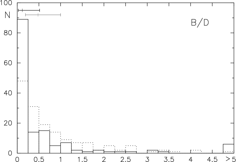
Figure 1: Bulge-to-disk ratio histogram of the UCM Survey in the Johnson $B$ band. In this plot and hereafter, the median value and first quartiles of the data will be shown at the top. Black lines correspond to $B$ band results; dotted lines for the histograms and grey lines for the median and error bars will refer to the Gunn $r$ data from now on

In Figs. 2, 3, 4 and 5, we show the histograms for the bulge and disk parameters $\mu_{e}^{c}$, $r_{e}$, $\mu_{0}^{c}$ and $d_{L}^{c}$, respectively. Scales are in kpc and surface brightnesses in mag$\cdot$arcsec^-2. Superindex $c$ denotes correction for Galactic extinction and inclination (in the disk typical surface brightness).

The averaged $\mu_{e}^{c}$ value is 22.8$\pm$2.3 mag$\cdot$arcsec^-2 (22.7$\pm$2.3 mag$\cdot$arcsec^-2 if we only take into account the galaxies with B/D$<$1.7, the low B/D subsample hereafter), typical for a late-type spiral (Kent Ke85 (1985); Simien Si89 (1989)). The typical scale of the bulge is in average 2.7 kpc (2.2 kpc for the low-B/D subsample), with a great dispersion ($\sigma$=4.8), but also common for a Sb-Sc galaxy. These values are very similar to the ones measured in the Gunn $r$ images, although there seems to be a lack of small bulges in the red data.

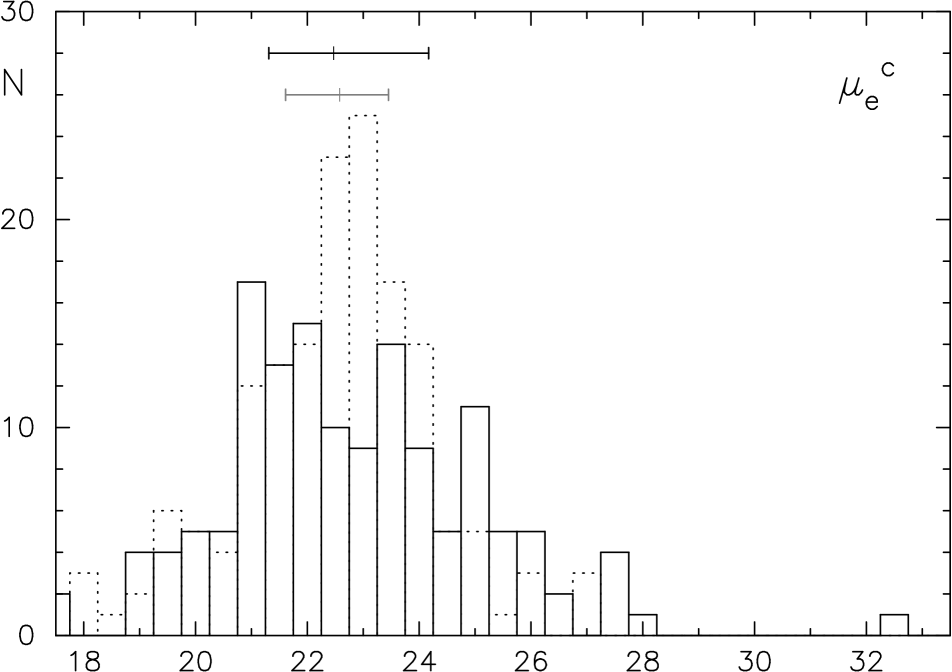
Figure 2: Histogram of the effective bulge surface brightness $\mu_{e}^{c}$ corrected for Galactic extinction

Figure 3: Histogram of the effective radius of the bulge component in kpc

The histogram of the characteristic surface brightness of the disk (Fig. 4) is dominated by galaxies with $\mu_{0}^{c}$=21-22 mag$\cdot$arcsec^-2, with the average in 21.1$\pm$1.1 mag$\cdot$arcsec^-2 (21.2$\pm$1.1 mag$\cdot$arcsec^-2 for the low-B/D subsample). The narrow range of $\mu_{0}^{c}$ seems to support the existence of a universal central surface brightness for the disk, as proposed for normal spirals by Freeman (Fre70 (1970)) and confirmed by other authors (i.e., Boroson Bo81 (1981), Simien & de Vaucouleurs Si86 (1986)), although other works in the literature present samples of galaxies with a wider spread in $\mu_{0}^{c}$ (see, for example, McGaugh et al. McG95 (1995) or Beijersbergen et al. Bei99 (1999)). Our $\mu_{0}^{c}$ value is $\sim 0.5^{m}$ brighter than the Freeman central surface brightness. Therefore, the UCM sample of star-forming galaxies appears to have brighter disks than those of normal spirals; this fact is probably related to the higher star-formation activity. Scale lengths are dominated by disks smaller than 4 kpc (68% of the total number of galaxies fitted), with mean 3.6$\pm$2.6 kpc (the same for the low-B/D subsample). This value is higher than that found by Chitre et al. (Chi99 (1999)) for a sample of starburst galaxies in the Markarian sample ($d_{L}^{c}<$3 kpc), very similar to the averaged value found by Vennik et al. (Ven00 (2000)) for a sample of emission-line galaxies ($d_{L}^{c}$$\sim$2.7 kpc), although they only fit an exponential to the outer parts of the profiles. Our value is lower than the one found by de Jong (1996a ) for normal edge-on spirals ($d_{L}^{c}$$\sim$8 kpc) -they argue that their selection biases against galaxies with low surface brightness and short scale lengths are large-. Other works (for example, Boroson Bo81 (1981), Kent Ke85 (1985), Bothun et al. Bot89 (1989), Andredakis & Sanders And94 (1994)) agree in placing our galaxies in the zone of short disk spirals, though one should be cautious against comparing scale lengths from different authors due to the subjective nature of disk parameters (Knapen & van der Kruit Kna91 (1991) find discrepancies up to a factor of two in the scale lengths calculated from several authors).

All of the above values are very similar to those found by Vitores et al. (1996b ) and place the UCM sample of galaxies in the zone of the late-type spirals, with small bulges and not very extended disks (Freeman Fre70 (1970)). Three remarks are interesting when comparing both sets of data. First, in the Gunn $r$ decomposition a lower bulge scale cut-off was observed (at $r_{e}$=0.5 kpc); this is not present in the $B$ band study. A possible explanation is the different handling performed with the seeing that allows the $B$ bulges to be smaller but brighter (seeing correction smoothes the profile; this was not the case with the Gunn $r$ bulge-disk decomposition, where the seeing effect was not taken into account directly), but this does not seem to cope with the whole difference. Second, both bands present a preference for disk scales around 2-3 kpc (larger disks in the blue band); very short disk scales and large ones are less frequent. Third, the difference between the surface brightness levels of the bulge and disk are of the order of the mean colour, around 0.5^m, as expected according to the averaged $B-r$ colour found in Fukugita et al. (Fuk95 (1995)).

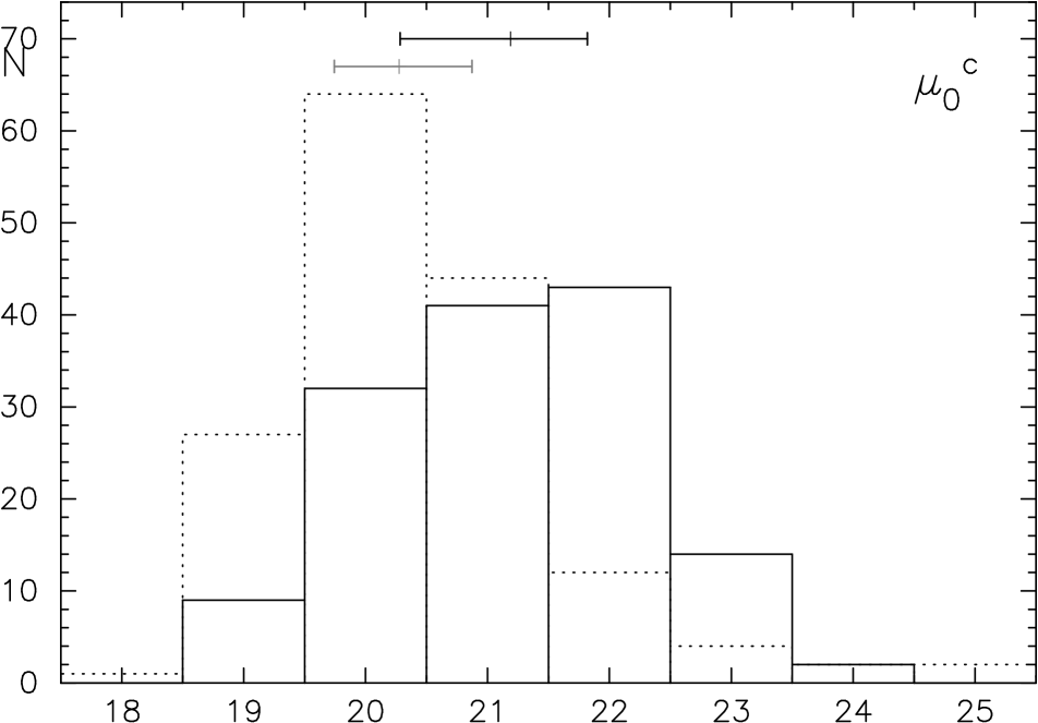
Figure 4: Histogram of the characteristic surface brightness of the disk $\mu_{0}^{c}$ corrected for Galactic extinction and inclination

Figure 5: Histogram of the exponential scale length of the disk $d_{L}^{c}$ measured in kpc

4.2 Geometric parameters

In order to typify the size of the UCM galaxies, the histograms representing the diameter of the 24.5 mag$\cdot$arcsec^-2 isophote D_24.5 and the effective radius $a_{e}$ (both in kpc) have been plotted in Figs. 6 and 7. The averaged diameter of the UCM objects is 22$\pm$12 kpc. Comparison with the red data has been established through the plot of the diameter of the 24 mag$\cdot$arcsec^-2 Gunn $r$ isophote (that will be nearer to the 24.5 blue isophote than the corresponding red one, assuming a mean colour $B-r\sim 0.5$). The mean effective radius $a_{e}$ is 3.8$\pm$2.3 kpc; this reflects the high degree of spatial luminosity concentration of our objects, most of them being starburst nuclei with a large emission arising from the center of the galaxy. Tentatively, UCM galaxies seem to be more extended in the blue band than in the red one (they show larger effective radius and diameters in $B$).

Figure 6: Histogram of the diameter of the 24.5 mag$\cdot$arcsec^-2 D_24.5 isophote in kpc

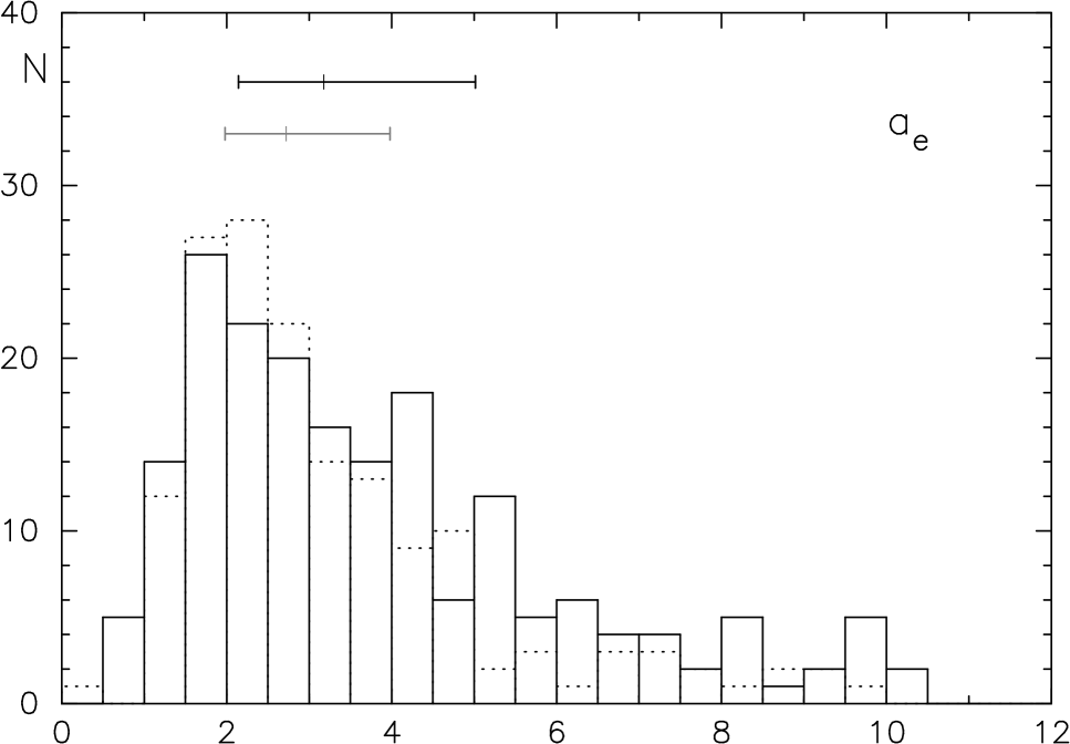
Figure 7: Histogram of effective radius $a_{e}$ in kpc

Finally, we plot in Figs. 8 and 9 the mean effective and isophote 24.5 surface brightnesses in order to characterize the whole galaxy luminosity distribution. UCM objects show $<\mu_{e}^{c}>$=21.2$\pm$0.9 and $<\mu_{24.5}^{c}>$=22.5$\pm$0.4 (both in mag$\cdot$arcsec^-2), common value for normal galaxies (Doi et al. Doi93 (1993)). The difference between the Gunn $r$ and the Johnson $B$ values ($\sim$0.5^m) is a common $B-r$ colour for spirals (Fukugita et al. Fuk95 (1995)).

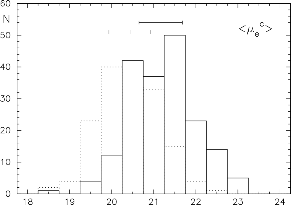
Figure 8: Histogram of the mean surface brightness inside the effective aperture $<\mu_{e}^{c}>$ corrected for Galactic extinction

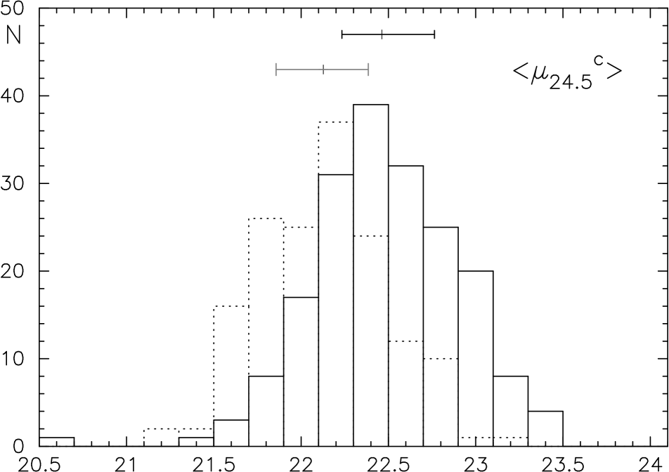
Figure 9: Histogram of the mean surface brightness inside the 24.5 isophote $<\mu_{24.5}^{c}>$ corrected for Galactic extinction

4.3 Concentration indices and asymmetry coefficient

In the next 3 figures, labelled 10, 11 and 12, histograms of the concentration indices are shown. Mean values are c_in=0.41$\pm$0.12, c₃₁=3.4$\pm$1.0 and c₄₂=3.3$\pm$0.6. All of them are common values for spiral galaxies, corresponding approximately to a Hubble type of Sb (Doi et al. Doi93 (1993), Gavazzi et al. Gav90 (1990), Kent Ke85 (1985), respectively for each concentration index). These values are higher than those measured in the Gunn $r$ images. The $B$ luminosity seems to be more concentrated in the inner parts than the $r$ one, although galaxies are more extended.

Fig. 13 depicts the histogram of the asymmetry coefficient for the UCM sample. The UCM sample is dominated by intermediately asymmetrical galaxies with mean 0.10$\pm$0.08, lower than the value found by Bershady et al. (Ber00 (2000)) for a sample of normal local galaxies; this could be due to a difference in the calculation of $A$ or because their sample is composed by bright, large objects which probably have many asymmetrical features. This is what we should expect for spirals which have a certain axis symmetry although they present arms, bars or HII regions that enlarge the asymmetry coefficient. There is a lack of highly symmetrical objects, which correspond to elliptical galaxies, not present in our sample as it is composed by star-forming systems.

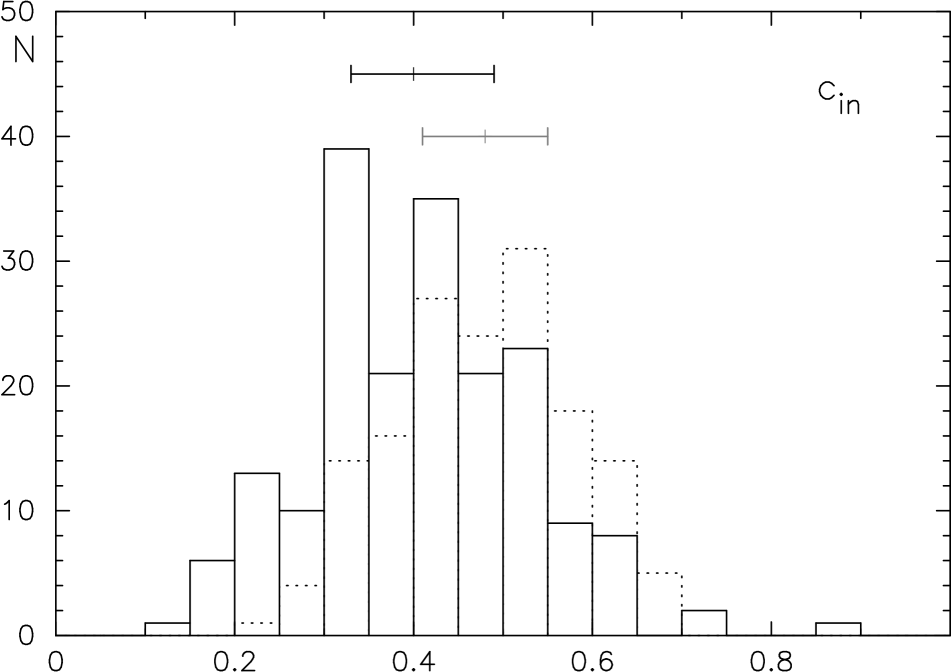
Figure 10: Histogram of the concentration index c_in of the UCM sample

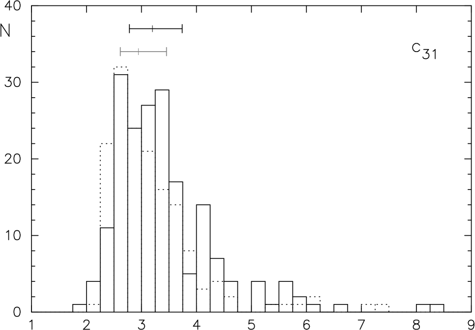
Figure 11: Histogram of the concentration index c₃₁ of the UCM sample

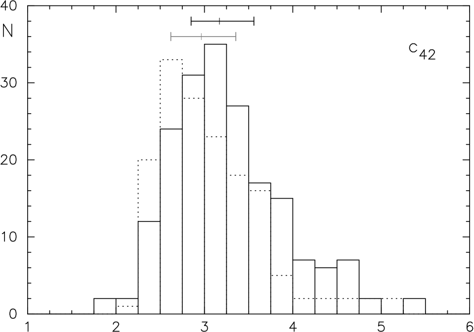
Figure 12: Histogram of the concentration index c₄₂ of the UCM sample

Figure 13: Histogram of the asymmetry coefficient $A$ of the UCM sample calculated after Abraham et al. Ab96a (1996)

All the previous results have been summarized in Table 3 for a quick look, jointly with the Gunn $r$ statistics.

Table 3: Mean, median and standard deviation of the photometric parameters of the Johnson $B$ and Gunn $r$ (in brackets) images of the UCM Survey galaxies (scales are in kpc and surface brightnesses in mag$\cdot$arcsec^-2)

Magnitudes	symbol	mean	st. dev.	median
Magnitudes
apparent magnitude	mB	16.1 (15.5)	1.1 (1.0)	16.1 (15.5)
absolute magnitude	MB	$-$19.9 ($-$20.5)	1.1 (1.1)	$-$20.0 ($-$20.6)
B+D parameters
bulge-to-disk ratio	B/D	0.40 (0.82)	0.65 (0.98)	0.12 (0.48)
effective bulge surface brightness	$\mu_{e}^{c}$	22.8 (22.6)	2.3 (1.7)	22.5 (22.6)
effective radius of the bulge	$r_{e}$	2.7 (2.1)	4.8 (3.3)	1.0 (2.1)
disk face-on central surface brightness	$\mu_{0}^{c}$	21.1 (20.3)	1.1 (1.1)	21.2 (20.3)
exponential scale length of the disk	$d_{L}^{c}$	3.6 (1.8)	2.6 (1.6)	3.0 (1.8)
Geometric parameters
diameter of the 24.5 mag$\cdot$arcsec-2 isophote	D24.5	22 (18)	12 (9)	19 (16)
Mean photometric parameters
effective radius	$a_{e}$	3.8 (3.3)	2.3 (1.9)	3.2 (2.7)
mean effective surface brightness	$<\mu_{e}^{c}>$	21.2 (20.4)	0.9 (0.7)	21.2 (20.4)
isophote 24.5 mag$\cdot$arcsec-2 mean surface brightness	$<\mu_{24.5}^{c}>$	22.5 (22.1)	0.4 (0.4)	22.5 (22.1)
Concentration indices
concentration index ($\alpha=0.3$)	cin	0.41 (0.48)	0.12 (0.10)	0.40 (0.48)
concentration index	c31	3.4 (3.2)	1.0 (0.9)	3.2 (3.0)
concentration index	c42	3.3 (3.1)	0.6 (0.6)	3.2 (3.0)
Asymmetry coefficient
asymmetry coefficient	$A$	0.10 (-)	0.08 (-)	0.09 (-)

4.4 Morphological classification

A morphological classification of the UCM galaxies has been carried out using 5 different criteria. These criteria were already used by Vitores et al. (1996a ) with the Gunn $r$ images, and are now applied to the Johnson $B$ data in order to compare the results obtained with different bandpasses. Besides, some galaxies not studied in Vitores et al. (1996a ) have now been classified for the first time (15% of the sample). We outline the main features of the classification criteria:

• the correlation between B/T ratio and Hubble type. B/T is defined as:

  $$B/T=\frac{1}{(B/D)^{-1}+1}$$ (9)

  This correlation was studied by Kent (Ke85 (1985), Fig. number 6) for a sample of bright galaxies in a red filter. It has been assumed that the behaviour of the correlation is very similar in the blue band.

• the dependence of the Hubble type on the position in the plane defined by the concentration index c${}_{in}(\alpha)$ and $\mu_{24.5}^{c}$, first studied by Doi et al. (Doi93 (1993)). These authors argue that this criterium is rather insensitive to the colour band.

• the correlation between the concentration index c₃₁ and the Hubble type, as studied by Gavazzi et al. (Gav90 (1990), Fig. 4b).

• the dependence of the morphological type on the concentration index c₄₂, established by Kent (Ke85 (1985), Fig. 11).

• the correlation between the mean surface brightness inside the effective isophote (corrected for Galactic extinction) and the Hubble type (Kent Ke85 (1985), Fig. 13). A mean correction of 0.5^m due to the different bandpasses used in both works has been applied.

Visual inspection of each image was also used for the classification.

In this work we utilized all these five criteria to classify the UCM galaxies in S0, Sa, Sb, Sc+ (Sc type or later) and Irr galaxies plus the BCD type (these galaxies were classified using spectroscopic confirmation available in Gallego et al. Gal96 (1996)); some galaxies were very distorted due to interactions and are marked in the result table as an independent class. The final Hubble type was established as that in which most criteria agree. This method is not completely objective and constitutes the main reason for the discrepancy between the classification using the Gunn $r$ data and that performed in this paper with the Johnson $B$ images. Table LABEL:morph presents the final classification in both bands. Fig. 14 shows the histograms and plots of the 5 criteria used in the classification; in these plots the general trend of each parameter with the Hubble type can be seen, although great scatter and overlap between the different types are also present. Mean values will be shown in Table 7.

Table 6 presents the number of UCM galaxies of each type in the Gunn $r$ and Johnson $B$ filters. A total number of 35 galaxies have been classified differently in the two bands, although the differences are always from one type to the contiguous (except in UCM2316+2028). Based on the Johnson $B$ data, 65% of the whole sample is classified as Sb or later (61% based on Gunn $r$ images). The percentage of barred galaxies is very similar in both bands (Johnson $B$ 9%, Gunn $r$ 8%); most of them are late-type spirals (47 % are Sb galaxies and 35 % Sc+). We have marked 6 clear interactions among the UCM galaxies (3%), although there are more objects with tails or structures that could have been formed during an interaction. Seyfert 1 galaxies (6 objects) are all classified as S0, except one (UCM0003+1955) that is very bright and could not be classified; Sy 2 galaxies have been classified as Sa (1 object), Sb (3 objects) and Sc+ (3 objects). These results are consistent with the ones found in the literature (see, for example, Hunt & Malkan Hun99a (1999)).

Table 4: Morphological classification of the UCM sample of galaxies

UCM name	MpT($B$)	MpT ($r$)	UCM name	MpT($B$)	MpT ($r$)	UCM name	MpT($B$)	MpT ($r$)
(1)	(2)	(3)	(1)	(2)	(3)	(1)	(2)	(3)
0000+2140	INTER	—	0141+2220	Sa	Sb	1314+2827	Sa	Sa
0003+2200	Sc+	Sc+	0142+2137	SBb	SBb	1320+2727	Sb	Sb
0003+2215	Sc+	—	0144+2519	SBc+	SBc+(r)	1324+2926	BCD	BCD
0003+1955	—	—	0147+2309	Sa	Sa	1324+2651	INTER	—
0005+1802	Sb	—	0148+2124	BCD	BCD	1331+2900	BCD	BCD
0006+2332	Sb	—	0150+2032	Sc+	Sc+	1428+2727	Irr	Sc+
0013+1942	Sc+	Sc+	0156+2410	Sb	Sc+	1429+2645	Sb	Sc+
0014+1829	Sa	Sa	0157+2413	Sc+	Sc+	1430+2947	S0	S0
0014+1748	SBb	SBb	0157+2102	Sb	Sb	1431+2854	Sb	Sb
0015+2212	Sa	Sa	0159+2354	Sb	Sa	1431+2702	Sa	Sb
0017+1942	Sc+	Sc+	0159+2326	Sc+	Sc+	1431+2947	BCD	BCD
0017+2148	Sa	—	1246+2727	Irr	—	1431+2814	Sb	Sa
0018+2216	Sb	Sb	1247+2701	Sc+	Sc+	1432+2645	SBb	SBb
0018+2218	Sb	—	1248+2912	SBb	—	1440+2521S	Sb	Sb
0019+2201	Sb	Sc+	1253+2756	Sa	Sa	1440+2511	Sb	Sb
0022+2049	Sb	Sb	1254+2741	Sb	Sb	1440+2521N	Sb	Sa
0023+1908	Sc+	—	1254+2802	Sc+	Sc+	1442+2845	Sb	Sb
0034+2119	SBc+	—	1255+2819	Sb	Sb	1443+2714	Sa	Sa
0037+2226	SBc+	—	1255+3125	Sa	Sa	1443+2844	SBc+	SBc+
0038+2259	Sb	Sa	1255+2734	Sc+	Irr	1443+2548	Sc+	Sc+
0039+0054	Sc+	—	1256+2717	S0	—	1444+2923	S0	S0
0040+0257	Sb	Sc+	1256+2732	INTER	—	1452+2754	Sb	Sb
0040+2312	Sc+	—	1256+2701	Sc+	Irr	1506+1922	Sb	Sb
0040+0220	Sc+	Sb	1256+2910	Sb	Sb	1513+2012	Sa	S0
0040$-$0023	Sc+	—	1256+2823	Sb	Sb	1537+2506N	SBb	SBb
0041+0134	Sc+	—	1256+2754	Sa	Sa	1537+2506S	SBa	SBa
0043+0245	Sc+	—	1256+2722	Sc+	Sc+	1557+1423	Sb	Sb
0043$-$0159	Sc+	—	1257+2808	Sb	Sa	1612+1308	BCD	BCD
0044+2246	Sb	Sb	1258+2754	Sb	Sb	1646+2725	Sc+	Sc+
0045+2206	INTER		1259+2934	Sb	Sb	1647+2950	Sc+	Sc+
0047+2051	Sc+	Sc+	1259+3011	Sa	Sa	1647+2729	Sb	Sb
0047$-$0213	S0	Sa	1259+2755	Sa	Sa	1647+2727	Sb	Sa
0047+2413	Sa	Sa	1300+2907	Sa	Sb	1648+2855	Sa	Sa
0047+2414	Sc+	—	1301+2904	Sb	Sb	1653+2644	INTER	—
0049$-$0006	BCD	BCD	1302+2853	Sb	Sa	1654+2812	Sc+	Sc+
0049+0017	Sb	Sc+	1302+3032	Sa	—	1655+2755	Sc+	Sb
0049$-$0045	Sb	—	1303+2908	Irr	Irr	1656+2744	Sa	Sa
0050+0005	Sa	Sa	1304+2808	Sb	Sa	1657+2901	Sb	Sc+
0050+2114	Sa	Sa	1304+2830	BCD	BCD	1659+2928	SB0	SB0
0051+2430	Sa	—	1304+2907	Irr	Irr	1701+3131	S0	S0
0054$-$0133	Sb	—	1304+2818	Sc+	Sc+	2238+2308	Sa(r)	Sa
0054+2337	Sc+	—	1306+2938	SBb	Sb	2239+1959	S0	S0
0056+0044	Irr	Irr	1306+3111	Sc+	Sc+	2249+2149	Sb	Sa
0056+0043	Sb	Sc+	1307+2910	SBb	SBb	2250+2427	Sa	Sa
0119+2156	Sb	Sc+	1308+2958	Sc+	Sc+	2251+2352	Sc+	Sc+
0121+2137	Sc+	Sc+	1308+2950	SBb	SBb	2253+2219	Sa	Sa
0129+2109	SBc+	—	1310+3027	Sb	Sa	2255+1930S	Sb	Sb
0134+2257	Sb	—	1312+3040	Sa	Sa	2255+1930N	Sb	Sb
0135+2242	S0	S0	1312+2954	Sc+	Sc+	2255+1926	Sb	Sc+
0138+2216	Sc+	—	1313+2938	Sa	Sa	2255+1654	Sc+	Sc+

Table 5: continued

UCM name	MpT($B$)	MpT ($r$)	UCM name	MpT($B$)	MpT ($r$)	UCM name	MpT($B$)	MpT ($r$)
(1)	(2)	(3)	(1)	(2)	(3)	(1)	(2)	(3)
2256+2001	Sc+	Sc+	2313+1841	Sb	Sb	2325+2318	INTER	—
2257+2438	S0	S0	2313+2517	Sa	—	2325+2208	SBc+	SBc+
2257+1606	S0	—	2315+1923	Sb	Sa	2326+2435	Sb	Sa
2258+1920	Sc+	Sc+	2316+2457	SBa	SBa	2327+2515N	Sb	Sb
2300+2015	Sb	Sb	2316+2459	Sc+	Sc+	2327+2515S	S0	S0
2302+2053W	Sb	Sb	2316+2028	Sa	Sc+	2329+2427	Sb	Sb
2302+2053E	Sb	Sb	2317+2356	Sa	Sa	2329+2500	S0(r)	S0(r)
2303+1856	Sa	Sa	2319+2234	Sb	Sc+	2329+2512	Sa	Sa
2303+1702	Sc+	Sc+	2319+2243	S0	S0	2331+2214	Sb	Sb
2304+1640	BCD	BCD	2320+2428	Sa	Sa	2333+2248	Sc+	Sc+
2304+1621	Sa	Sa	2321+2149	Sc+	Sc+	2333+2359	S0a	S0
2307+1947	Sb	Sb	2321+2506	Sc+	Sc+	2348+2407	Sa	Sa
2310+1800	Sb	Sc+	2322+2218	Sc+	Sc+	2351+2321	Sb	Sb
2312+2204	Sa	—	2324+2448	Sb	Sc+

Table 5: (1) UCM name. (2) Morphological type established using 5 different criteria based on luminosity concentration and bulge-disk decomposition applied to the Johnson $B$ images. (3) Morphological type established using 5 different criteria based on luminosity concentration and bulge-disk decomposition applied to the Gunn $r$ images

Table 6: Hubble types for the UCM galaxies

Filter	S0	Sa	Sb	Sc+	Irr	BCD	Int	Total
$B$	14	38	69	50	5	8	6	190
	7%	20%	36%	26%	3%	4%	3%
$r$	12	41	43	46	5	8	$-$	155
	7%	27%	28%	30%	3%	5%

Table 6: Number of galaxies and percentage of the UCM galaxies according to their Hubble type in the Johnson $B$ and the Gunn $r$ bandpasses

5 Correlations between parameters

We plot in Figs. 15 and 16 the relationships between absolute $B$ magnitude and the size of the galaxy (24.5 isophote diameter) and also between M_B and the distribution of light (concentration index c₃₁). Information about morphological classification is also shown.

There is a tight correlation between M_B and D_24.5. A least-square fit to our data leads to:

$$log\,D_{24.5}=(-2.65\pm 0.16)+(-0.20\pm 0.01)\,M_{B}$$ (10)

The slope is very similar to the value expected for a constant luminosity-area ratio ($log\,D=C-0.2\,M$). Therefore, despite there is a great variety in morphological and spectroscopic types, a uniformity in the mean surface brightness is exhibited, as was also proved with the red data (Vitores et al. 1996b found a slope value of $-$0.21$\pm$0.01). The fit gives a mean surface brightness value of $-$13.3 mag$\cdot$kpc^-2.

In Fig. 16 a general trend between the concentration index c₃₁, the absolute $B$ magnitude M_B and the morphological type is apparent. Early-type galaxies show medium-high magnitudes and high concentration indices. If we move downwards to the zone of low concentration index we find spirals, from Sa to late-type. Finally, BCDs have c₃₁ values typical for spirals but are fainter than normal galaxies.

Fig. 17 shows the segregation in morphological type in a c_in versus A diagram. In this plot and the next, median values for the different morphological types are plotted with a black dot; ellipse semi-axes are the $\sigma$ of each parameter. There is a clear trend from left to right in decreasing Hubble type. S0 galaxies are placed in the high symmetry-high c_in zone. BCDs also appear as highly symmetrical objects. On the other hand, irregulars are shown as highly asymmetrical objects in the top-left zone of the plot and interactive systems are located among the most asymmetrical galaxies. A trend can be also remarked in the spiral sequence: early-type galaxies are more symmetrical than late-type ones (due to the presence of more HII regions, for example).

Figure 15: Relationship between the size of the UCM galaxies represented by the diameter of the 24.5 isophote D_24.5 and the total $B$ luminosity of the object M_B. A least-square fit to the data is also plotted

Figure 16: Concentration index c₃₁ versus absolute magnitude M_B. Different symbols stand for distinct morphological types

Figure 17: Concentration index c_in versus asymmetry coefficient. Different symbols stand for distinct morphological types. Ellipses show the median and standard deviation of each parameter for the different morphological types

Fig. 14 showed that there is a clear correlation between the concentration indices and Hubble type. This trend is also observed with the asymmetry coefficient. Table 7 presents the mean values of the bulge-to-disk ratio, mean effective surface brightness, concentration indices and asymmetry coefficient of each Hubble type. The statistics of $A$ have been split into barred and non-barred objects; barred galaxies are more asymmetrical than non-barred ones.

Table 7: Averaged values of each Hubble type

Parameter	S0	Sa	Sb	Sc+	Irr	BCD	Int
B/T	0.53	0.39	0.16	0.04	0.07	0.41	0.30
$\mu_{e}$	20.6	20.7	21.3	21.5	21.8	21.5	20.1
c31	5.3	3.8	3.3	2.7	2.9	3.5	5.0
c42	4.3	3.5	3.2	2.7	2.8	3.4	4.0
cin	0.58	0.50	0.40	0.29	0.33	0.35	0.57
A	0.09	0.10	0.10	0.11	0.21	0.06	0.20
(barred)	0.06	0.15	0.11	0.12	$-$	$-$	$-$

Fig. 18 depicts the absolute $B$ magnitude of the UCM objects versus the mean effective surface brightness. Early-type galaxies appear as bright, high surface brightness objects. Late-type spirals have lower $\mu_{e}$, although no significant difference in M_B is present. BCDs are clearly segregated due to their faintness. Irregulars and interactive systems show also a distinctive surface brightness.

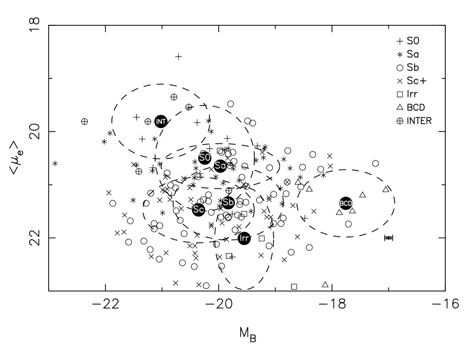
Figure 18: Mean effective surface brightness versus absolute magnitude. Ellipses show the median and standard deviation of each parameter for the different morphological types

6 Summary and conclusions

We have carried out a morphological study of the UCM Survey galaxies based on Johnson $B$ imaging. This paper, jointly with Paper I (Pérez-González et al. yor (2000)), have analyzed the main features of the UCM sample concerning integrated and surface photometry in the $B$ bandpass.

Paper I presented integrated apparent and absolute $B$ luminosities as well as isophote 24 mag$\cdot$arcsec^-2 magnitudes. Effective radii and $B-r$ colours were also calculated in this first release. In the present paper we have outlined the main results concerning bulge-disk decomposition values, ellipticities, position angles, concentration indices, mean photometric radii and surface brightnesses and asymmetry coefficients.

All the above information has been used to perform the morphological classification of the UCM galaxies. The sample is dominated by late Hubble type objects (65% being Sb or later). We have not found a great difference between this classification and the results achieved with the Gunn $r$ data (Vitores et al. 1996a , 1996b ).

Our galaxies are characterized by shorter disks than those of normal spirals. Besides, they seem to be objects with a high luminosity concentration. A preliminary comparison between the characteristics of the sample in the red and blue bandpasses, yields to the result that emission-line galaxies have a higher concentration of blue light than red light in the inner parts of the objects; on the contrary, they also seem to be more extended in $B$ than in $r$.

Finally, a size-luminosity correlation has been outlined. We have also presented several plots where a morphological segregation is patent. These plots involve information about luminosity, concentration of light and asymmetry.

In next papers we will face a most exhaustive comparison between bands, including colour gradients and a stellar population study. Likewise, we will likened our sample to high-redshifts surveys searching for clues to their nature and galaxy evolution.

Figure 14: Plots of the 5 criteria used to morphologically classify the UCM galaxies. Top panels show on the left the distribution of the B/T ratio and on the right the mean effective surface brightness (corrected for Galactic extinction) according to the final Hubble type established for each galaxy. The middle panel shows the plot found in Doi et al. (Doi93 (1993)) of concentration index c_in versus isophote 24.5 mean surface brightness; the dashed line represents the segregation between late-type and early-type established by Doi et al. (Doi93 (1993)). Lower panels are the histograms of the concentration indices c₄₂ (left) and c₃₁ (right)

- (1) Abraham R.G., van den Bergh S., Galzebrook K., et al., 1996, ApJS 107, 1
- (2) Alonso-Herrero A., Aragón-Salamanca A., Zamorano J., Rego M., 1996, MNRAS 278, 417
- (3) Alonso O., García-Dabó E., Zamorano J., Gallego J., Rego M. 1999, ApJS 122, 415
- (4) Andredakis Y.C., Sanders R.H., 1994, MNRAS 267, 283
- (5) Baggett W.E., Baggett S.M., Anderson K.S.J., 1998, AJ 116, 1626
- (6) Bershady M.A., Jangren A., Conselice C.J., 2000, AJ 119, 2645
- (7) Beijersbergen M., de Blok W.J.G., van der Hulst J.M., 1999, A&A 351, 903
- (8) Bothun G.D., Halpern J.P., Lonsdale C.J., Impey C., Schmitz M., 1989, ApJS 70, 271
- (9) Boroson T., 1981, APJS 46, 177
- (10) Chitre A., Joshi U.C., 1999, A&AS 139, 105
- (11) Chatzichristou E.T., 1999, astro-ph/9912227
- (12) de Jong R.S., 1996a, A&A 313, 45
- (13) de Jong R.S., 1996b, A&AS 118, 557
- (14) de Vaucouleurs G., 1948, Ann. d’Ap., 11, 247
- (15) de Vaucouleurs G., 1977, Evolution of galaxies and stellar populations, eds. Larson R.B., & Tynsley B.M., New Haven, Yale Univ. Obs., 43
- (16) Doi M., Fukugita M., Okamura S., 1993, MNRAS 264, 832
- (17) Freeman K.C., 1970, ApJ, 160, 811
- (18) Fukugita M. Shimasaku K., Ichikawa T., 1995, PASP 107, 945
- (19) Gallego J., Zamorano J., Aragón-Salamanca A., Rego M., 1995, ApJ 455, L1
- (20) Gallego J., 1999, Ap&SS 263, 1
- (21) Gallego J., Zamorano J., Rego M., Alonso O., Vitores A. G., 1996, A&AS 120, 323
- (22) Gallego J., Zamorano J., Rego M., Alonso O., Vitores A. G., 1997, ApJ 475, 502
- (23) Gavazzi G., Garilli B., Boselli A., 1990, A&AS 83, 399
- (24) Gil de Paz A., Aragón-Salamanca A., Gallego J., et al., 2000, MNRAS 316, 357
- (25) Hu E.M., Cowie L.L., McMahon R.G., 1998, ApJ 502, 99
- (26) Hunt L.K., Malkan, M.A., 1999, ApJ 516, 660
- (27) Hunt L.K., Malkan M.A., Moriondo G., Salvati M., 1999, ApJ 510, 637
- (28) Jedrzejewski P., 1987, MNRAS 226, 747
- (29) Knapen J.H., van der Kruit P.C., 1991, A&A 248, 57
- (30) Kent S.M., 1985, ApJS 59, 115
- (31) Kron R.G., 1980, ApJS 43, 305
- (32) McGaugh S.S., Bothun G.D., Schombert J.M., 1995, AJ 110, 573
- (33) Pérez-González P.G., Zamorano J., Gallego J., Gil de Paz A., 2000, A&AS, 141, 409
- (34) Pritchet C., Kline M.I., 1981, AJ 86, 1859
- (35) Schombert J.M., Bothun G.D., 1987, AJ 93, 60
- (36) Simien F., 1989, Photometric decomposition of galaxies. In: Corwin H.G., & Bottinelli L. (eds.) The World of Galaxies. Springer-Verlag, N. York, page 293
- (37) Simien F., de Vaucouleurs G., 1986, ApJ 282, 95
- (38) Steidel C.C., Adelberger K.L., Giavalisco M., Dickinson M., Pettini M., 1999, ApJ 519, 1
- (39) Vennik J., Hopp U., Popescu C.C., 2000, A&AS 142, 399
- (40) Vitores A.G., Zamorano J., Rego M., Alonso O., Gallego J., 1996a, A&AS 118, 7
- (41) Vitores A.G., Zamorano J., Rego M., Gallego J., Alonso O., 1996b, A&AS 120, 385
- (42) Zamorano J., Rego M., Gallego J., et al.,1994, ApJS 95, 387
- (43) Zamorano J., Gallego J., Rego M., Vitores A.G., Alonso O., 1996, ApJS 105, 343