Radial and Transverse Velocities of Nearby Galaxies

Abstract

Analysis of the peculiar velocities of galaxies should take account of the uncertainties in both redshifts and distances. We show how this can be done by a numerical application of the action principle. The method is applied to an improved catalog of the galaxies and tight systems of galaxies within 4$h_{75}^{-1}$ Mpc, supplemented with a coarser sample of the major concentrations at 4$h_{75}^{-1}$ Mpc to 20$h_{75}^{-1}$ Mpc distance. Inclusion of this outer zone improves the fit of the mass tracers in the inner zone to their measured redshifts and distances, yielding best fits with reduced $\chi^{2}$ in redshift and distance in the range 1.5 to 2. These solutions are based on the assumption that the galaxies in and near the Local Group trace the mass, and a powerful test would be provided by observations of proper motions of the nearby galaxies. Predicted transverse galactocentric velocities of some of the nearby galaxies are confined to rather narrow ranges of values, and are on the order of 100 km s^-1, large enough to be detected and tested by the proposed SIM and GAIA satellite missions.

1. Introduction

This paper continues the analysis of the dynamics of relative motions of the galaxies in and near the Local Group. In previous numerical applications of the action principle either the present distances of the assumed mass tracers are given, and the measure of goodness of fit is the difference between model and catalog redshifts (Peebles 1989), or the present redshifts are given, and the measure of goodness of fit is the difference between model and catalog distances. Since errors in redshift and distance both are important we have adapted the numerical action method to allow relaxation to a stationary point of the action and a minimum of the sum of the squares of the weighted differences of model and catalog redshifts and distances. The method is described in § 3.

In § 4 we present an application of the method to the catalog discussed in § 2. Recent advances in measurements of distances of nearby galaxies are incorporated in a catalog of the distances and radial velocities of the galaxies and tight concentrations of galaxies within 4$h_{75}^{-1}$ Mpc. (Hubble’s constant is $H_{o}=75h_{75}$ km s^-1 Mpc^-1). This inner zone catalog is supplemented by a coarser catalog of distances and radial velocities of the main galaxy concentrations in an outer zone at 4–20$h_{75}^{-1}$ Mpc distance. We work with the assumption that the luminosities of the galaxies trace the mass. Two control cases support this assumption: (i) inclusion of the outer zone in the dynamical solutions improves the fit to the measured redshifts and distances in the inner zone, and (ii) replacing the angular positions by random positions on the sky, while keeping the catalog redshifts and distances, worsens the fit.

The application presented here is meant to illustrate the new numerical method and catalogs; we hope to present a systematic study of parameters in a later paper. With the parameter choices for cosmology and mass-to-light ratios ($M/L$, using blue-band light) listed in § 4 we get values of the reduced $\chi^{2}$ for distances and redshifts that in the best cases are between 1.5 and 2, close enough to unity to add to the evidence that our model is a useful approximation to reality. A considerably stronger test, from measurements of transverse motions of nearby galaxies, is discussed in § 5.

2. Catalogs of Nearby Galaxies

Our compilation of mass tracers and potential targets for measurements of proper motions is restricted by three considerations. (1) Accurate distances are needed to constrain models. (2) In this first exploration of the method we want to restrict the number of orbits to reconstruct. (3) Complex — strongly nonlinear — orbits can only be recovered with an extensive exploration of initial conditions. The first two led us to study about 40 objects. The third compels the merging of some closely adjacent galaxies into single entries in our catalog.

Regarding the last point, it is possible in principle to find numerical action solutions in cases where galaxies have already made close passages, as long as there has not been significant exchange of orbital and internal energy. For example, the interactions between M81, M82, and NGC 3077 left extended tidal streams of neutral hydrogen that provide detailed constraints on the relative motions (Yun, Ho, & Lo 1994), a case that would be fascinating to study. However, the current work has a much less ambitious goal. If galaxies are so near to each other that the orbits may be complex, we merge the information on these systems: the catalog entries are the sums of the luminosities and the luminosity-weighted positions and velocities. What is meant by ‘near to each other’ depends on the available information. For galaxies that are close to us we have better relative discrimination of positions and a more complete census of the major mass influences. Consequently, we attempt to explore somewhat more complex situations in the nearest volume.

Our catalog has ‘inner’ and ‘outer’ zones. The former, within 4$h_{75}^{-1}$ Mpc distance, is the main sample in this study. About $90\%$ of the light in the inner zone resides in just 8 of the objects. If mass and light are strongly correlated then most of the inner catalog mass is associated with these few giant systems. It is important for the dynamical analysis that these few big objects be located as precisely as possible in position and velocity. The many small galaxies make a minor contribution to the light and, we are assuming, to the mass. We seek to include as many of these objects as feasible because they are valuable probes of the gravitational potential, but their exclusion would have little effect on the dynamics. Thus we include all the massive galaxies in the inner zone, whatever the reliability of their distance estimates, but only dwarfs that are sufficiently isolated to have simple orbits and for which we have good distance estimates.

Thanks especially to the Hubble Space Telescope, reasonably good distances are emerging for many galaxies in and at the fringe of the Local Group. Two techniques are providing most of the data: the correlation between pulsation period and luminosity of Cepheid variable stars (eg., Freedman et al. 1994) and the calibrated luminosity of the tip of the Red Giant Branch for evolved low-metallicity stars (eg., Cole et al. 1999). Each can provide distances with 10% standard deviation. There is a further 10% uncertainty in the underlying zero points, but this normalization is close to a common factor in all distances and so enters only as a scale factor in the dynamics. The distance scale used in this paper is consistent with H${}_{\circ}=75$ km s^-1 Mpc^-1 (Tully & Pierce 2000; Tonry et al. 2000); a zero point shift is accommodated by the factor $h_{75}={\rm H}_{\circ}/75$. Distance measurement coverage of individual galaxies falls rapidly beyond 4$h_{75}^{-1}$ Mpc.

Some comments on the characteristics of the nearby structure are in order. Almost all galaxies within 1$h_{75}^{-1}$ Mpc have negative systemic velocities, which suggests this region is gravitationally bound but not yet relaxed. The galaxies in this region make up the Local Group. This condensation is part of an expanding filamentary structure, with the nearest big galaxies close to each other in the sky in what are called the Maffei–IC342 and M81 groups. The filament originates in the northern Galactic hemisphere at a conjunction of filaments near the Ursa Major and Coma I clusters, passes through small knots of galaxies in the constellations of Canes Venatici and Ursa Major, through our position, and can be followed in the southern Galactic hemisphere out to the NGC 1023 Group. The thread of galaxies that makes up what has been called the Sculptor Group can be viewed as a minor fragment of the main filament. It seems this filament is paralleled by a second one that originates in the Galactic north at the Virgo Cluster, passes through a big knot including the Sombrero galaxy, then passes nearest to us at the Centaurus Group, through the Galactic plane in the vicinity of Circinus galaxy, and onward to meet with the Telescopium-Grus Cloud. Tully & Fisher (1987) provide maps of these structures.

The outline of these features can be seen in Figure 1, though in skeleton form because we have plotted only the important dynamical constituents and those that serve as useful test particles. Our inner zone catalog in Table 1 is shown as the filled symbols. This sample is thought to be complete in luminous objects ($L_{B}>10^{10}~{}L_{\odot}$) within 4$h_{75}^{-1}$ Mpc, and we are assuming it is a good sample of the mass. The unnamed objects are dwarfs with decent distance measurements. All the inner zone objects are concentrated near the equatorial plane in supergalactic coordinates. If light traces mass the major gravitational influence on the Local Group from the inner zone is the Maffei/IC342/M81 complex, with some influence from the Centaurus Group, a minor effect from the modest galaxies in the Sculptor Group, and little else. There are no important mass elements near the boundary of the inner zone. This degree of isolation and the sharp decline in the completeness of distance measurements led us to place the boundary for the main inner zone at 4$h_{75}^{-1}$ Mpc.

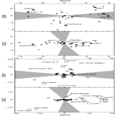
Figure 1.— Projected locations of catalog objects. Top pair of panels: Region within $\pm 4h_{75}^{-1}$ Mpc from two orthogonal viewpoints in supergalactic coordinates. Bottom pair of panels: Region within $\pm 20h_{75}^{-1}$ Mpc from the same orthogonal viewpoints. Shaded wedges identify zones of Galactic obscuration.

Gravitational interactions with more distant mass concentrations affect the dynamics within our inner zone. The nearest substantial exterior concentrations of galaxies are at distances of 15–20$h_{75}^{-1}$ Mpc. Then at 30–60$h_{75}^{-1}$ Mpc there are still larger concentrations in the Norma-Hydra-Centaurus and Perseus-Pisces supercluster regions. For this paper we ignore the big structures beyond $30h_{75}^{-1}$ Mpc but try to account for the significant structures within an outer zone at 4–$20h_{75}^{-1}$ Mpc distance. The distribution of important galaxy concentrations in this outer zone is simple enough to be modeled by the 14 objects in Table 2. These groups or clusters (numerical names from Tully 1988) are shown as open symbols in Figure 1, and the eight that cause the largest gravitational tides at our position (based on mass divided by distance cubed) are identified by name in the bottom pair of panels in the figure.

The Virgo Cluster is not an outstandingly dominant contributor to the local luminosity, but there is good evidence that it is a larger contributor to the mass. Numerical action modeling, which mostly refers to the low density environments where most galaxies are found, indicates the cosmological mass density parameter is $\Omega_{m}=0.25\pm 0.2$ (95% formal probable error) with mass-to-light ratio $M/L\sim 150h_{75}~{}M_{\odot}/L_{\odot}$ in typical galaxy environments (Shaya, Peebles, & Tully 1995; Tully 1999). The evidence that there is much more mass in the Virgo Cluster than would be inferred from this value of $M/L$ includes the velocity dispersions of the early and late-type galaxies near the core, the high velocities of galaxies infalling on first approach to the cluster (Tully & Shaya 1984; 1998), and the virgocentric flow derived from the distances in the surface brightness fluctuations survey (Tonry et al. 2000). Tully & Shaya (1998) conjecture that the Virgo Cluster is not the only nearby place where $M/L$ is large, that regions with short dynamical times ($t_{collapse}\sim 10^{9}$ years) have high $M/L$, and that such regions are readily identified as nests of elliptical and S0 galaxies. It is argued that these regions have $M/L$ at least five times that of regions with long dynamical times ($t_{collapse}\sim 10^{10}$ years). If so, four other systems with large $M/L$ within 20$h_{75}^{-1}$ Mpc are the E/S0 knots associated with the Fornax, Dorado, Coma I, and Leo clusters/groups. These entities are located by large boxes in the bottom two panels of Figure 1; we assign them $M/L$ five times that of the nine low density groups with long dynamical times and mainly late-type galaxies in the outer zone. The most massive of the low $M/L$ members of the outer zone, the Sombrero and Ursa Major clusters, are identified by the larger open circles in Figure 1. The NGC 6946 group is the nearest of the outer zone systems at 6$h_{75}^{-1}$ Mpc (a distance that still is quite uncertain).

The mass we assign to the Virgo Cluster is four times that of the second most massive system in Table 2, and larger than the sum of all the other masses within 20$h_{75}^{-1}$ Mpc. A simple measure of the interactions among inner and outer zone objects is given in the last column in Table 2: the relative contribution of each outer object to the present tidal field at our position. One sees again the importance of the Virgo cluster, and the not insignificant sum of contributions from the rest of the outer zone objects.

The luminosities of all the galaxies in the outer zone that are not in the 14 objects in Table 2 add up to a luminosity density that is comparable to the cosmic mean used by Shaya, Peebles, & Tully (1995). That is, the 14 mass tracers in the outer zone approximate the overdensity of luminosity, and plausibly of mass, within 20$h_{75}^{-1}$ Mpc.

Our numerical analysis assumes distance measurement errors are symmetrically distributed in the distance moduli, with the standard deviations $\sigma_{\mu}$ listed in Tables 1 and 2. The standard deviations $\sigma_{cz}$ in the redshifts in Table 1 are measurement errors, while the $\sigma_{cz}$ listed in Table 2 are mean deviations of the velocity dispersions within these clusters and groups of galaxies. A crude model for the motion of each galaxy relative to the dark halo it is supposed to trace is presented in § 4.

The objects near the outer boundary of the outer zone likely are strongly influenced by structures beyond 20$h_{75}^{-1}$ Mpc that are not in our analysis. Hence although orbit computations are constrained by the distances and velocities, with their uncertainties, in both zones, the solutions are evaluated only from the fits to the redshifts and distances in the inner zone.

3. Solutions that Minimize $\chi^{2}$

3.1. Numerical Action Method

This initial discussion, for simplicity, deals with a single particle. A solution to the equation of motion generally has neighboring solutions with neighboring values of the present distance and redshift, and we seek the member of this family that minimizes

$$\chi^{2}=(z-z_{c})^{2}/\sigma_{z}^{2}+(\mu-\mu_{c})^{2}/\sigma_{\mu}^{2},$$ (1)

where the redshift and distance modulus in the solution are $z$ and $\mu$, the measured catalog values are $z_{c}$ and $\mu_{c}$, and their standard deviations are $\sigma_{z}$ and $\sigma_{\mu}$. The relaxation of a single-particle orbit to stationary points of the action and of $\chi^{2}$ is applied separately to each member of the catalog and iterated until the gradients of the action and $\chi^{2}$ vanish to machine accuracy. Relaxation to a minimum of the sum of the $\chi^{2}$ over all particles (except the reference), rather than iterated relaxation to minima of single-particle $\chi^{2}$, is feasible but the matrix inversion is a considerably heavier computation.

We represent the orbit of a particle by its comoving positions ${\bf x}_{n}$ at a sequence of time steps $t_{n}$, $1\leq n\leq n_{x}$, together with the present distance $d$ at time $t_{o}=t_{n_{x}+1}$ and given present angular position, as in Peebles (1995). The action function is

$$A=S+H_{o}d^{2}/2-d(cz+{\bf v}_{\rm MW}\cdot\hat{x}),$$ (2)

where

$$S = \sum_{n=1}^{n_{x}}{a_{n+1/2}^{2}\over 2}{({\bf x}_{n+1}-{\bf x}_{n})^{2}\over(t_{n+1}-t_{n})}$$ (3)

$$- (t_{o}-t_{n_{x}+1/2})V_{o}$$

$$- \sum_{n=1}^{n_{x}}(t_{n+1/2}-t_{n-1/2})V_{n}.$$

The term $S$ approximates the time integral of the kinetic minus the potential energies. The potential for particle $i$ is

$$V=-G\sum_{j\not=i}{m_{j}\over a(t)x_{ji}}-{\Omega H_{o}^{2}a_{o}^{3}{\bf x}_{i}^{2}\over 4a}.$$ (4)

The physical distance between particles $i$ and $j$ is $a(t)x_{ij}$. The second term in $V$ refers the potential to the background cosmological model with present Hubble constant $H_{o}$ and density parameter $\Omega$ in matter with mass density that varies inversely as the cube of the expansion parameter $a(t)$. The terms added to $S$ in equation (2) represent a canonical transformation that in effect exchanges radial positions and momenta, thereby changing the boundary condition from fixed present distance to fixed present radial velocity (the details of which are presented in Phelps 2000). The present radial velocity of the particle relative to the Milky Way is $cz$, and the last term in equation (2) adds the component of the peculiar velocity ${\bf v}_{\rm MW}$ of the Milky Way in the direction $\hat{x}$ of the particle. (The velocities are such that the center of mass moves according to eq. [7] in Peebles 1994). The derivative of the action with respect to the present distance is

$${\partial A\over\partial d} = {a_{n_{x}+1/2}^{2}\over a_{o}}{\hat{x}\cdot({\bf x}_{o}-{\bf x}_{n_{x}})\over t_{o}-t_{n_{x}}}$$ (5)

$$- (t_{o}-t_{n_{x}+1/2}){\partial V_{o}\over\partial d}$$

$$+ H_{o}d-cz-{\bf v}_{\rm MW}\cdot\hat{x}.$$

The first term on the right hand side is the radial canonical momentum of the particle a half time step before the present, where $\hat{x}$ is the unit vector to the present particle position. The second term brings the radial momentum to the present epoch. When $\partial A/\partial d=0$ this agrees with the radial peculiar velocity given by the last three terms. One similarly sees that the conditions $\partial A/\partial{\bf x}_{n}=0$ represent the equation of motion in leapfrog approximation (Peebles 1995). The motion of the Milky Way is at a stationary point of the function $S$ of the coordinates of this orbit, with the boundary condition that the Milky Way ends up at the origin.

To simplify discussion of the relaxation to stationary points of $A$ and $\chi^{2}$ let $x_{\alpha}$ represent the $3n_{x}+1$ coordinates for the orbit of a particle (or the $3n_{x}$ coordinates for the Milky Way), with $\alpha=0$ for the present distance $x_{0}=d$. The first and second derivatives of the action with respect to these variables are $A_{\alpha}$ and $A_{\alpha\beta}$. The square of the gradient of the action for particle $i$ is $\Gamma_{i}=\sum(A_{\alpha})^{2}$. The coordinate shift

$$\delta x_{\alpha}=-\epsilon\sum_{\beta}A^{-1}{}_{\alpha\beta}A_{\beta}$$ (6)

reduces $\Gamma_{i}$ if $\epsilon$ is small enough. If $x_{\alpha}$ is close to a stationary point, so $A$ is close to a quadratic function of the distance from the stationary point, then $\epsilon=1$ brings the orbit much closer to the stationary point, whether a local extremum or saddle point.

Now consider neighboring stationary points of the action, where $A_{\alpha}=0$, belonging to neighboring redshifts $z$ and $z+dz$. The result of differentiating $A_{\alpha}=0$ with respect to $z$, and remembering that the coordinates $x_{\alpha}$ are functions of redshift and that $z$ also appears explicitly in $A_{0}$ (eq. [5]) is

$$A_{\alpha\beta}{\partial x_{\beta}\over\partial z}=c\delta_{\alpha,0}.$$ (7)

We see that in a family of solutions related by continuously varying the redshift $z$ the derivative of the present distance $d$ with respect to the redshift is

$${\partial d\over\partial z}=cA^{-1}{}_{00}.$$ (8)

The inverse of the matrix of second derivatives of $A$ thus shows how to move the orbit toward a stationary point of $A$ (eq. [6]) and how the present distance at a stationary point of $A$ changes when the redshift is adjusted. We use the latter to relax to a minimum of $\chi^{2}$. The derivative of $\chi^{2}$ (eq. [1]) with respect to the redshift satisfies

$$\sigma_{z}^{2}{\partial\chi^{2}\over\partial z}/2=z-z_{c}+R{\partial d\over\partial z}{\ln d/d_{c}\over d},$$ (9)

where

$$R=\left({5\over 2.303}{\sigma_{z}\over\sigma_{\mu}}\right)^{2}.$$ (10)

We find that it is a good numerical approximation to suppose $\partial d/\partial z$ is independent of $z$. In this case the second derivative satisfies

$$\sigma_{z}^{2}{\partial^{2}\chi^{2}\over\partial z^{2}}/2=1+{R\over d^{2}}\left(\partial d\over\partial z\right)^{2}(1-\ln d/d_{c}).$$ (11)

The analog of equation (6) for a redshift adjustment that moves the orbit toward the minimum of $\chi^{2}$ is

$$\delta z=-\epsilon{\partial\chi^{2}/\partial z\over\partial^{2}\chi^{2}/\partial z^{2}}.$$ (12)

To sample the families of solutions we start from random orbits with the positions ${\bf x}_{n}$ at $1\leq n\leq n_{x}$ placed independently at random in the sphere that contains the mass of the system of objects in the background cosmological model. The iterative relaxation first uses the matrix inverse $A^{-1}{}_{\alpha\beta}$ to find $\partial d/\partial z$ and hence the redshift adjustment $\delta z$ (and the accompanying adjustment to $\partial A/\partial d$) that moves the orbit toward a minimum of $\chi^{2}$, and then uses the same matrix inverse to find the coordinate adjustments $\delta x_{\alpha}$ that move the orbit toward a stationary point of $A$.

3.2. Numerical Fixes

We expect colleagues who wish to explore applications of this method would do well to seek independent ways to address the numerical problems arising, so as to improve our inelegant and likely inefficient fixes, but to aid reproducing our results we list the main elements of our procedure.

The square of the gradient of the action summed over all objects $i$ and position coordinates $\alpha$ is

$$\Gamma=\sum_{i}\Gamma_{i}=\sum_{i,\alpha}(\partial A/\partial x_{i,\alpha})^{2}.$$ (13)

With the velocity unit 100 km s^-1, length unit 1 Mpc, and mass unit $1\times 10^{11}$ solar masses, the square of the gradient of the action for the initial random orbits typically is $\Gamma\sim 10^{8}$. At $\Gamma\lesssim 10^{-10}$ further iterations usually reduce the square of the gradient of $A$ to zero to machine accuracy (32 bit) without appreciable perturbations to the orbits. In the solutions presented here the iteration stops at $\Gamma\sim 10^{-20}$, at which point $(\partial\chi^{2}/\partial z)^{2}$ is similarly small. The iteration can approach a point where $\Gamma$ has a local minimum but not a zero. In our experience when this happens $\Gamma$ is dominated by the contribution from one object, so when $\Gamma_{i}>\Gamma/2$ for object $i$ its orbit alone is adjusted until $\Gamma_{i}<0.01\Gamma$ or to a maximum of 300 iterations. If this happens for particle $i$ more than 100 times we choose a new random orbit for the object and relax it alone until $\Gamma_{i}<0.01\Gamma$. Negative distances, and orbits that cross at zero separation, are unphysical but allowed by the mathematics. During the relaxation a distance can move from negative to positive, so when object $i$ has distance $d_{i}<30$ kpc and $\Gamma_{i}<1$ we choose a new random orbit for this object and relax it until $\Gamma_{i}<0.01\Gamma$. When $\Gamma<1$ and the minimum comoving separation of a pair of particles is less than 30 kpc we apply the above procedure to the less massive one. Equation (8) assumes the coordinates are at a stationary point of $A$, but we apply the redshift adjustment at each coordinate adjustment starting from random orbits. When the coordinates are far from a stationary point the approximation to $\partial^{2}\chi^{2}/\partial z^{2}$ in equation (11) can be negative. In this case we relax down the gradient of $\chi^{2}$, using

$$\delta z=-\epsilon{\chi^{2}\over\partial\chi^{2}/\partial z},$$ (14)

When the second derivative of $\chi^{2}$ is positive we use the smaller of the redshift adjustments from equations (12) and (14). There are many solutions to the equation of motion for the objects in Tables 1 and  2; we seek those with redshifts and distances that are close to the catalog values. When the relaxation brings $\Gamma$ below $10^{-5}$ each object in turn with individual $\chi^{2}$ greater than 25 is given 40 attempts at a new orbit, relaxed from a random one, to bring the individual $\chi^{2}$ below 25. After this treatment of each offending orbit all orbits are iteratively relaxed until $\Gamma<10^{-5}$ again. The operation is repeated, allowing a maximum of 5 sets of 40 attempts for each object. In the analysis of the real catalogs usually all individual $\chi^{2}$ are below 25 after about 1000 iterations through all orbits. In the control case with randomly placed present angular positions the allowed number of attempts usually is exhausted by 1000 iterations, leaving some objects with quite large $\chi^{2}$. At $n_{x}>10$ time steps the computation time scales as $n_{x}^{3}$, dominated by the matrix inversion codes LUDCMP and LUBKSB from Press et al. (1992).

4. Application to the Nearby Galaxies

4.1. Parameters and Control Samples

In this illustration of the numerical method we fix some parameters by considerations other than the motions of the nearby galaxies. We adopt a cosmologically flat Friedmann-Lemaître model with matter density and Hubble parameters

$$\Omega_{m}=0.25,\qquad H_{\circ}=75h_{75}\hbox{ km s}^{-1}~{}\hbox{Mpc}^{-1}.$$ (15)

Our choice of $\Omega_{m}$ is near the lower end of the range derived from recent measurements of the angular fluctuations in the thermal cosmic background radiation (eg. Hu et al. 2000) and near the upper end from analyses of galaxy dynamics (as summarized by Tully & Shaya 1998 and Bahcall et al. 2000). The value of $H_{\circ}$ fits the recession velocities of galaxies at $cz=5000$ to 8000 km s^-1 that plausibly are in the Hubble flow (Tully & Pierce 2000). The scale factor $h_{75}$ takes account of a close to common uncertainty in the distance zero points for $H_{o}$ and the distances in Tables 1 and 2.

Luminosities are computed at the catalog distances. The masses in the inner zone in Table 1 assume the mass-to-light ratio

$$M/L({\rm inner})=75h_{75}~{}M_{\odot}/L_{\odot}.$$ (16)

This choice makes the sum of the masses of M31 and the Milky Way consistent with the spherical model for their relative motion, and the total mass contrast at $r<4h_{75}^{-1}$ Mpc is $\delta M/\langle M\rangle=1.0$, consistent with the modest gravitational slowing of the local expansion rate just outside the Local Group. Following the discussion in § 2, we take account of the light in the outer zone that is not in the mass concentrations in Table 2 by adopting a larger mass-to-light ratio,

$$M/L({\rm outer})=150h_{75}~{}M_{\odot}/L_{\odot},$$ (17)

for the late-type systems in Table 2, and $750h_{75}~{}M_{\odot}/L_{\odot}$ for the early type systems. This makes the contrast $\delta M/\langle M\rangle=0.6$ at $r<20h_{75}^{-1}$ Mpc, again a reasonable number.

To take account of the distributed mass around the tracers we change the first term in the gravitational potential in equation (4) to $V\propto(x_{ij}{}^{2}+(c_{i}+c_{j})^{2})^{-1/2}$, with comoving cutoff length $c_{i}=30$ kpc for all particles in the inner zone, 2 Mpc for Virgo, and 700 kpc for all other objects in the outer zone. The cutoff is larger in the outer zone because these objects are meant to represent more broadly distributed mass. When all cutoff lengths are set to zero it allows more sharply curved and perhaps unphysical orbits, but the statistics are little changed.

The standard deviations $\sigma_{\rm cz}$ in redshift take account of the dispersions of velocities in the large systems of galaxies in Table 2, but in Table 1 reflect only the measurement errors. Since we can only guess at the typical difference between the velocity of the galaxy and the motion of the center of mass of the dark halo it is supposed to represent, we write the standard deviation in redshift as

$$\sigma_{z}=(\sigma_{cz}^{2}+\sigma_{o}^{2})^{1/2},$$ (18)

and we compare results for $\sigma_{o}=0$ and $c\sigma_{o}=15$ km s^-1.

We label dynamical solutions for the combined set of orbits of the objects in both zones as c0 and c15, for the two values of $\sigma_{o}$. In the first set of control cases, labeled i0 and i15, the outer zone has been removed from the dynamics. In the second set of control cases, labeled r0 and r15, the outer zone is included and the catalog distances and redshifts are used but each object is placed at a randomly chosen position in the sky (with the same angular position in all solutions). All statistics for all cases are based on the objects in the inner zone alone.

We use $n_{x}=20$ time steps uniformly spaced in the expansion parameter $a(t)$ and $\epsilon=0.2$ in the relaxation equations (6), (12), and (14). The statistics are quite similar at $\epsilon=0.1$ and $\epsilon=0.3$, and at $n_{x}=15$ and $n_{x}=30$. We compute 30 solutions from random orbits for each case.

Figure 2.— Distributions of reduced $\chi^{2}$ in distance and redshift for 30 solutions for each of the six cases. In the broken histograms $\sigma_{o}=0$, in the solid, $c\sigma_{o}=15$ km s^-1.

4.2. Numerical Solutions

Figure 2 shows the distributions of reduced $\chi^{2}$ in redshift and distance summed over the 29 objects in the inner zone (excluding the Milky Way) for the 30 solutions for each of the six cases. Increasing the standard deviations in the redshifts makes it considerably easier to find solutions with reduced $\chi^{2}$ less than 3. Removing the outer zone from the dynamics or scrambling the angular positions makes it more difficult to find these relatively good fits to the data. The differences of the best $\chi^{2}$ among the 30 solutions for each case are much smaller than the differences among the distributions of $\chi^{2}$ from all 30 solutions, but the best solution for the real catalogs is consistently better than the best solution for the control cases.

Figure 3.— Distributions of normalized differences between model and catalog redshifts and distance moduli in the best solutions for cases c0 (filled squares) and r0 (open squares).

The last two columns in Table 1 and the filled squares in Figure 3 show the normalized differences between model and catalog redshifts and distances for the 29 objects in the best solution for the real catalogs with $\sigma_{o}=0$ (case c0). For comparison we show as the open symbols the normalized differences in the best of the solutions for scrambled angular positions (case r0). The normalized scatter is smaller in redshift and correlated with the scatter in distance. This is because $\partial d/\partial z$ (eq. [8]), the rate of change of redshift with respect to distance in a family of solutions, usually is positive and, in the units in Figure 3, the slope usually is greater than unity. The single-particle $\chi^{2}$ are minimized at the closest approach of the trajectory of redshift as a function of distance to the origin in Figure 3, so the minima scatter around a line that trends down to the right. Some trajectories happen to pass close to the origin in Figure 3; their relaxation to minimize $\chi^{2}$ produces unrealistically good fits to the catalog redshifts and distances.

Figure 4.— Distributions of single-particle $\chi^{2}$ in redshift and distance modulus for the 29 objects in the solutions with the smallest total $\chi^{2}$ for each case. In the broken histograms $\sigma_{o}=0$, in the solid, $\sigma_{o}=15$ km s^-1.

Figure 4 shows the distributions of single-particle $\chi^{2}$ in redshift and distance for the best solutions for each of the six cases. (To avoid confusion we note that Fig. 2 is the distribution of total $\chi^{2}$ among 30 solutions, while Fig. 4 is the distribution of single-particle $\chi^{2}$ for the 29 objects in the best solution for each case.) To reduce the spread of values we plot the square root of the sum of the squares of the normalized differences of model and catalog redshifts and distances. The curve is the distribution for Gaussian normal scatter of the redshifts and distances. There tend to be more objects with $\chi^{2}<1$ than expected for this idealized model, even in the random case. This is a result of the relaxation to minimize $\chi^{2}$, as discussed in connection with Figure 3. Even in the best solution for the real data there are more large values of $\chi^{2}$ than expected from the idealized distribution, but the excess is not large. For example, in c0 there are 10 of the 29 objects with $\chi^{2}>4$, about 2.5 times the number expected from the idealized model.

Our computation allows many attempts to find an acceptable fit to catalog redshifts and distances, and the fit may be achieved at the expense of an unrealistic initial condition, associated with an unacceptable value or gradient of the primeval mass density fluctuation. Estimates of the primeval density fluctuations associated with a numerical action solution are discussed in Peebles (1996). We use a simplified approach based on the linear perturbation relation between the mass density contrast $\delta$ and the peculiar velocity field ${\bf v}({\bf x})$,

$${\partial\delta\over\partial t}=-{1\over a}\nabla\cdot{\bf v}.$$ (19)

This expression averaged over a sphere of comoving radius $x$ is $\dot{\delta}=-3v_{r}/ax$, where $v_{r}$ is the peculiar velocity normal to and averaged over the surface of the sphere. The density contrast at high redshift varies as $\delta\propto D(t)$, where $D(t)$ is the growing solution to the linear perturbation equation, so an estimate of the local density contrast extrapolated to the present in linear perturbation theory is

$$\delta_{o}=-3{D_{o}\over\dot{D}(t)}{(\dot{\bf x}_{i}-\dot{\bf x}_{j})\cdot({\bf x}_{i}-{\bf x}_{j})\over x_{ij}^{2}}.$$ (20)

The dot means derivative with respect to proper world time $t$, $D_{o}$ is the present value of $D$, and ${\bf x}_{i}$ and $\dot{\bf x}_{i}$ are the coordinate position and velocity of particle $i$ at time $t$. We use the approximation $\dot{\bf x}=({\bf x}_{3}-{\bf x}_{2})/(t_{3}-t_{2})$, from the second to the third time step, because the fractional increase in time from the first to the second step is large, though it yields similar results.

Figure 5.— Distributions of estimates of the local primeval density contrast extrapolated to the present in linear perturbation theory (eq. [20]) in the best solutions for the six cases. The thin histograms assume $\sigma_{o}=0$, the thick, $c\sigma_{o}=15$ km s^-1.

Figure 5 shows distributions of $\delta_{o}$ from all pairs of objects in the inner catalog for the best solution for each of the six cases. When the outer zone is removed from the dynamics the central value of the contrast $\delta_{o}$ is close to unity, the value expected from the choice of $M/L$. The outer zone objects increase the central value of $\delta_{o}$ for the inner zone, we suspect because the inner and outer zone objects are somewhat intermingled at high redshift. There are substantial differences among the distributions from solutions with similar values of $\chi^{2}$; reproducible features include the smaller central value of $\delta_{o}$ when the outer zone is removed, the prominent positive tail in the distribution of $\delta_{o}$ from the real catalogs, and the still more prominent tails in the random case.

Because we have used a crude estimate of $\delta_{o}$, and lumped together a range of values of primeval separations $x_{ij}$, we could not expect the distributions in Figure 5 to be Gaussian even if we had an adequate approximation to Gaussian initial conditions. However, we might expect the more realistic cases to be closer to Gaussian. By this criterion the random control case is the least realistic, as we would hope. On the other hand, the outer zone increases the positive tail for the objects in the inner zone. This illustrates the difficulty of testing models at the present level of accuracy of the redshift and distance measurements. We turn now to a more demanding test.

Figure 6.— Transverse galactocentric velocity of M31 in all 30 solutions. The larger symbols have reduced total $\chi^{2}$ less than 2.5. Squares, crosses and triangles pointing up use the two zones, case c15. Diamonds, plus signs, and triangles pointing down show the effect of removing the outer zone. The symbol shapes are chosen according to $v_{\rm SGB}$, to facilitate comparison with the next 2 figures.

5. Proper Motions

The satellite missions SIM (http://sim.jpl.nasa.gov) and GAIA (http://astro.estec.esa.nl/GAIA) could measure the velocities of nearby galaxies relative to the Milky Way and perpendicular to the line of sight, and thereby test the assumption that the galaxies trace the local mass distribution.

Figures 6 to 8 show examples of transverse velocities in our 30 solutions The larger symbols represent the better fits to the catalog redshifts and distances, with reduced $\chi^{2}$ for the inner objects less then 2.5, the smaller symbols the solutions with larger $\chi^{2}$. The symbol orientations distinguish solutions with and without the outer zone objects in the dynamics, as explained in the caption to Figure 6.

When the dynamics includes only the inner catalog the transverse galactocentric velocity of M31 (Fig. 6) is close to zero in a few solutions, but in most cases M31 is moving at close to $\pm 150$ km s^-1 normal to the supergalactic plane. This is part of a collapse to the local sheet-like arrangement shown in Figure 1. When the outer zone objects are included in the dynamics the fit is improved, the solutions have a broader range of values of the transverse velocity, and there are more solutions with a near radial approach of M31. The better solutions still prefer motion toward the supergalactic plane, and there are many possible directions of transverse motion that could appear to falsify the action model.

Figure 7.— Transverse galactocentric velocity of IC 1613. The symbol shapes are chosen according to the value of ${\rm v_{SGB}}$ for M31, and the sizes according to the value of the total $\chi^{2}$, as in Fig. 6.

The distribution of solutions for the transverse galactocentric velocity of IC 1613 in Figure 7 is broader when the outer zone is included, as for M31. One might have expected to see a correlation of solutions for the velocities of M31 and this distant companion of M31. There is no pronounced correlation in this example, but we regard this as a very preliminary indication to be considered in more detail.

Figure 8.— Transverse galactocentric velocity of NGC 6822. The symbol shapes are chosen according to the value of ${\rm v_{SGB}}$ for M31 in Fig. 6, but here the larger symbols represent solutions in which the radial velocity of NGC 6822 is within 30 km s^-1 of the catalog value.

The orbit of NGC 6822 is more complex than M31 because NGC 6822 is closer and moving away. Figure 8 shows one can find acceptable fits to the catalog redshift and distance, with a broader range of possible proper motions than in the previous two examples. We suspect this illustrates a loss of memory of initial conditions in nonlinear classical dynamics. Tighter constraints on acceptable solutions might arise from a study of the initial conditions in the solutions; this also requires more study.

6. Discussion

6.1. The Assumption Galaxies Trace Mass

If the nearby galaxies trace the mass on scales $\gtrsim 100$ kpc then our inner catalog in Table 1 gives a reasonably complete description of the mass within 4$h_{75}^{-1}$ Mpc, and Table 2 gives a first approximation to the effect of external masses on the Local Group and its immediate neighbors. We have found dynamical solutions for the orbits of the assumed mass tracers that end up in our inner zone (within 4$h_{75}^{-1}$ Mpc distance); in the best cases the rms difference between model and catalog redshifts and distances is in the range 1.25 to 1.5 times the nominal catalog errors. The better fits use a more liberal estimate for the redshift errors, an issue that requires further consideration. The difference of the reduced $\chi^{2}$ from unity is considerably larger than statistical, but small enough to argue for the assumption galaxies trace mass.

One of our controls keeps the catalog distances, redshifts, and masses but places the objects at random positions in the sky. Since this preserves the near Hubble flow of the more distant members of the inner zone and the infall of most of the closer members, it is not surprising that we get a rough fit. But this scrambling of the present angular positions worsens the fit, as expected if galaxies trace mass. This result is quite stable under changes in the random numbers for the scrambling and computation.

Our second control removes the outer masses from the dynamics. It shows that the outer masses improve the fit to the measured redshifts and distances in the inner zone, again as expected if galaxies trace mass. This also suggests our solutions for the inner zone would be improved by using a better model for the external mass distribution, another point that requires further consideration.

Figures 6 to 8 show that, if galaxies trace mass, there are solutions with similar values of $\chi^{2}$ and transverse velocities that differ by 300 km s^-1. These solutions tend to occupy restricted regions of transverse velocity space. The predictions for the galactocentric transverse velocity of M31 are only weakly perturbed by the masses beyond 4$h_{75}^{-1}$ Mpc. Thus we suspect that under the assumption galaxies trace mass the allowed velocity of M31 is rather tightly constrained by the present catalogs. A measurement of the transverse velocity of this and other nearby galaxies could critically test the picture of the local mass distribution.

6.2. Comments on Future Work

This new version of the numerical action method could and certainly should be applied to numerical N-body simulations. We hope to continue work on this topic. Our exploration of the effect of adjusting the mass-to-light ratios in the data has been quite limited, and here too we hope to be able to report on the values of $M/L$ for late and early type systems that yield the best fit to catalog redshifts and distances, to compare to global measures of the density parameter.

The allowance for errors in both redshift and distance is more realistic than previous applications of the action method, but it still ignores the errors in masses. A study of this issue certainly will be part of a satisfactory assessment of the dynamics of the nearby galaxies.

A fundamental limitation of our numerical application should be noted. The matrix inverse of the second derivatives of the action with respect to the coordinates of an orbit gives the rate of change of the present distance with respect to the redshift (eq. [8]), and it reaches saddle points and local maxima as well as the local minima that are reached by following the gradient of the action. Because the computation time for the matrix inverse varies as the cube of the matrix size we relax the coordinates for each particle separately, toward a stationary point of the action and a minimum of the single-particle $\chi^{2}$. This is iterated through all particles many times. We are really interested in the minimum of the sum of the $\chi^{2}$ for all particles, which need not minimize any single-particle $\chi^{2}$. The inversion of the much larger matrix of all coordinates of all particles would be a heavy computation, but worth attempting.

The galaxy NGC 6822 illustrates the problem of dealing with complex orbits. We have found reasonably close fits to its positive radial velocity by relaxing from random orbits, but it would be feasible and useful to develop a more systematic sample of the many allowed orbits for such cases. The results would challenge us to decide which solutions could have come from realistic initial conditions; we need something better than the simple estimator in equation (20).

Table 1. Inner Catalog
Name	Note	SGL	SGB	distance	$\sigma_{\mu}$	redshift	$\sigma_{cz}$	mass	$\chi_{\mu}$	$\chi_{z}$
		(deg)	(deg)	(Mpc)		(km s${}^{-1})$	(km s${}^{-1})$	($\log_{10}[M_{\odot}$])
I342	+a	$10.8$	$0.3$	$3.6$	$0.59$	$171$	$5$	$12.5$	$2.0$	$-0.1$
Maffei	+b	$359.4$	$1.2$	$4.0$	$0.40$	$152$	$54$	$12.5$	$0.6$	$-0.4$
M31	+c	$335.5$	$11.1$	$0.8$	$0.16$	$-113$	$5$	$12.5$	$-1.6$	$1.0$
M81	+d	$41.1$	$0.7$	$3.7$	$0.17$	$114$	$6$	$12.4$	$-1.4$	$0.4$
N5128	+e	$161.6$	$-7.0$	$3.5$	$0.31$	$371$	$9$	$12.4$	$1.0$	$-0.2$
GALAXY		$-$	$-$	$-$	$-$	$-$	$-$	$12.3$	$-$	$-$
N253	+f	$272.6$	$-4.7$	$2.9$	$0.30$	$229$	$5$	$12.2$	$-0.8$	$0.1$
N5236	+g	$148.6$	$0.4$	$3.3$	$0.56$	$373$	$8$	$11.9$	$0.9$	$-0.1$
N2403	+h	$30.8$	$-7.5$	$3.3$	$0.20$	$227$	$5$	$11.8$	$4.1$	$-0.7$
N4236		$47.1$	$11.4$	$3.9$	$0.30$	$118$	$9$	$11.5$	$-3.8$	$1.0$
Circinus		$183.1$	$-6.4$	$3.3$	$0.80$	$268$	$9$	$11.5$	$-0.6$	$0.1$
N55	+i	$256.2$	$-2.4$	$1.6$	$0.30$	$96$	$5$	$11.5$	$-0.5$	$0.1$
N7793		$261.3$	$3.1$	$4.1$	$0.30$	$230$	$7$	$11.5$	$-2.4$	$0.3$
N300		$259.8$	$-9.5$	$2.1$	$0.20$	$101$	$5$	$11.3$	$-3.4$	$1.7$
N1569		$11.9$	$-4.9$	$2.4$	$0.60$	$47$	$5$	$11.0$	$0.7$	$0.0$
N404		$331.8$	$6.3$	$3.6$	$0.20$	$115$	$13$	$10.8$	$-0.6$	$0.2$
N3109	+j	$138.0$	$-45.1$	$1.3$	$0.17$	$194$	$5$	$10.5$	$-1.4$	$0.3$
IC5152		$234.2$	$11.5$	$1.7$	$0.20$	$85$	$9$	$10.0$	$-1.9$	$1.0$
SexA,B	+k	$102.6$	$-40.2$	$1.4$	$0.17$	$165$	$6$	$10.0$	$3.8$	$-1.3$
N6822		$229.1$	$57.1$	$0.5$	$0.17$	$45$	$6$	$10.0$	$-1.8$	$0.9$
N1311		$243.2$	$-34.3$	$3.1$	$0.40$	$425$	$15$	$9.8$	$2.0$	$-0.3$
IC1613		$299.2$	$-1.8$	$0.7$	$0.17$	$-155$	$5$	$9.8$	$-3.7$	$0.3$
WLM		$277.8$	$8.1$	$0.9$	$0.17$	$-65$	$5$	$9.7$	$-2.2$	$1.1$
VIIZw403		$36.9$	$11.4$	$4.5$	$0.20$	$50$	$7$	$9.6$	$-0.6$	$0.1$

Table 1. (Continued) Inner Catalog
Name	Note	SGL	SGB	distance	$\sigma_{\mu}$	redshift	$\sigma_{cz}$	mass	$\chi_{\mu}$	$\chi_{z}$
		(deg)	(deg)	(Mpc)		(km s${}^{-1})$	(km s${}^{-1})$	($\log_{10}[M_{\odot}$])
SagDIG		$221.3$	$55.5$	$1.1$	$0.20$	$7$	$7$	$9.1$	$0.4$	$-0.2$
PegDIG		$305.8$	$24.3$	$0.8$	$0.20$	$-22$	$5$	$8.9$	$-1.0$	$0.1$
LeoA		$69.9$	$-25.8$	$0.7$	$0.30$	$-18$	$7$	$8.8$	$0.7$	$-0.3$
DDO210		$252.1$	$50.2$	$0.9$	$0.20$	$-24$	$6$	$8.7$	$0.0$	$0.0$
DDO155		$103.0$	$4.7$	$1.5$	$0.40$	$183$	$5$	$8.6$	$-1.3$	$0.1$
Phoenix		$254.3$	$-20.9$	$0.4$	$0.20$	$-34$	$10$	$7.7$	$1.5$	$-1.6$

Notes to Table 1. The following galaxies are combined into single entries.

a) IC 342, NGC 1560, UGCA 105

b) Maffei 1, Maffei 2

c) M 31, M 33, IC 10, LGS 3

d) M 81, M 82, NGC 2976, IC 2574

e) NGC 5128 = Cen A, NGC 4945

f) NGC 253, NGC 247

g) NGC 5236 = M 83, NGC 5102

h) NGC 2403, NGC 2366, Holmberg II

i) NGC 55, ESO 294-010

j) NGC 3109, Antlia dwarf

k) Sextans A, Sextans B

References

- (1) Bahcall, N. A., Cen, R., Davé, R., Ostriker, J. P. & Yu, Q. 2000, astro-ph/0002310
- (2) Cole, A. A., et al. 1999, AJ, 118, 1657
- (3) Freedman, W.L., et al. 1994, ApJ, 427, 628
- (4) Giavalisco, M., Mancinelli, B., Mancinelli, P. J. & Yahil, A. 1993, ApJ, 411, 9
- (5) Hu, W., Fukugita, M., Zaldarriaga, M., & Tegmark, M. 2000, astro-ph/0006436
- (6) Peebles, P. J. E. 1989, ApJ, 344, L53
- (7) Peebles, P. J. E. 1994, ApJ, 429, 43
- (8) Peebles, P. J. E. 1995, ApJ, 449, 52
- (9) Peebles, P. J. E. 1996, ApJ, 473, 42
- (10) Phelps, S. D. 2000, dissertation Princeton University
- (11) Press, W. H., Teukolsky, S. A., Vetterling, W. T., & Flannery, B. P. 1992, Numerical Recipes, second edition, Cambridge Univerity Press
- (12) Schmoldt, I. M. & Saha, P. 1998, AJ, 115, 2231
- (13) Shaya, Edward J., Peebles, P. J. E., & Tully, R. Brent, 1995, ApJ, 454, 15
- (14) Tonry, J.L., Blakeslee, J.P., Ajhar, E.A., & Dressler, A. 2000, ApJ, 530, 625
- (15) Tully, R.B 1988, Nearby Galaxies Catalog, Cambridge University Press
- (16) Tully, R.B. 1999, in IAU Symp. 183: Cosmological Parameters and the Evolution of the Universe, ed. K. Sato (Reidel), p54 (astro-ph/9802026)
- (17) Tully, R.B & Fisher, J.R. 1987, Nearby Galaxies Atlas, Cambridge University Press
- (18) Tully, R.B. & Pierce, M.J. 2000, ApJ, 533, 744
- (19) Tully, R.B. & Shaya, E.J. 1984, ApJ, 281, 31
- (20) Tully, R.B. & Shaya, E.J. 1998, in Evolution of Large-Scale Structure, eds. A.J. Banday, R.K. Sheth, and L.N. Da Costa, p296 (astro-ph/9810298)
- (21) Whiting, A. B 2000, astro-ph/0002378
- (22) Yun, M. S., Ho, P. T. P., & Lo, K. Y. 1994, Nature, 372, 530