In the Beginning: The First Sources of Light
and the Reionization of the Universe

Abstract

The formation of the first stars and quasars marks the transformation of the universe from its smooth initial state to its clumpy current state. In popular cosmological models, the first sources of light began to form at a redshift $z=30$ and reionized most of the hydrogen in the universe by $z=7$. Current observations are at the threshold of probing the hydrogen reionization epoch. The study of high-redshift sources is likely to attract major attention in observational and theoretical cosmology over the next decade.

1 Preface: The Frontier of Small-Scale Structure

The detection of cosmic microwave background (CMB) anisotropies (Bennett et al.  1996; de Bernardis et al.  2000; Hanany et al.  2000) confirmed the notion that the present large-scale structure in the universe originated from small-amplitude density fluctuations at early times. Due to the natural instability of gravity, regions that were denser than average collapsed and formed bound objects, first on small spatial scales and later on larger and larger scales. The present-day abundance of bound objects, such as galaxies and X-ray clusters, can be explained based on an appropriate extrapolation of the detected anisotropies to smaller scales. Existing observations with the Hubble Space Telescope  (e.g., Steidel et al. 1996; Madau et al. 1996; Chen et al. 1999; Clements et al. 1999) and ground-based telescopes (Lowenthal et al. 1997; Dey et al. 1999; Hu et al. 1998, 1999; Spinrad et al. 1999; Steidel et al. 1999), have constrained the evolution of galaxies and their stellar content at $z\lesssim 6$. However, in the bottom-up hierarchy of the popular Cold Dark Matter (CDM) cosmologies, galaxies were assembled out of building blocks of smaller mass. The elementary building blocks, i.e., the first gaseous objects to form, acquired a total mass of order the Jeans mass ($\sim 10^{4}M_{\odot}$), below which gas pressure opposed gravity and prevented collapse (Couchman & Rees 1986; Haiman & Loeb 1997; Ostriker & Gnedin 1996). In variants of the standard CDM model, these basic building blocks first formed at $z\sim 15$–$30$.

An important qualitative outcome of the microwave anisotropy data is the confirmation that the universe started out simple. It was by and large homogeneous and isotropic with small fluctuations that can be described by linear perturbation analysis. The current universe is clumpy and complicated. Hence, the arrow of time in cosmic history also describes the progression from simplicity to complexity (see Figure 1). While the conditions in the early universe can be summarized on a single sheet of paper, the mere description of the physical and biological structures found in the present-day universe cannot be captured by thousands of books in our libraries. The formation of the first bound objects marks the central milestone in the transition from simplicity to complexity. Pedagogically, it would seem only natural to attempt to understand this epoch before we try to explain the present-day universe. Historically, however, most of the astronomical literature focused on the local universe and has only been shifting recently to the early universe. This violation of the pedagogical rule was forced upon us by the limited state of our technology; observation of earlier cosmic times requires detection of distant sources, which is feasible only with large telescopes and highly-sensitive instrumentation.

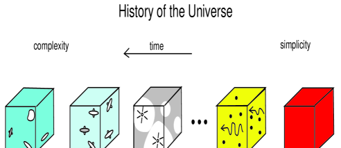
Figure 1: Milestones in the evolution of the universe from simplicity to complexity. The “end of the dark ages” bridges between the recombination epoch probed by microwave anisotropy experiments ($z\sim 10^{3}$) and the horizon of current observations ($z\sim 5$–6).

For these reasons, advances in technology are likely to make the high redshift universe an important frontier of cosmology over the coming decade. This effort will involve large (30 meter) ground-based telescopes and will culminate in the launch of the successor to the Hubble Space Telescope,  called Next Generation Space Telescope (NGST ). Figure 2 shows an artist’s illustration of this telescope which is currently planned for launch in 2009. NGST  will image the first sources of light that formed in the universe. With its exceptional sub-nJy ($1~{}{\rm nJy}=10^{-32}{\rm erg~{}cm^{-2}~{}s^{-1}~{}Hz^{-1}}$) sensitivity in the 1–3.5$\mu$m infrared regime, NGST  is ideally suited for probing optical-UV emission from sources at redshifts $\gtrsim 10$, just when popular Cold Dark Matter models for structure formation predict the first baryonic objects to have collapsed.

Figure 2: Artist’s illustration of one of the current designs (GSFC) of the Next Generation Space Telescope. More details about the telescope can be found at http://ngst.gsfc.nasa.gov/

The study of the formation of the first generation of sources at early cosmic times (high redshifts) holds the key to constraining the power-spectrum of density fluctuations on small scales. Previous research in cosmology has been dominated by studies of Large Scale Structure (LSS); future studies are likely to focus on Small Scale Structure (SSS).

The first sources are a direct consequence of the growth of linear density fluctuations. As such, they emerge from a well-defined set of initial conditions and the physics of their formation can be followed precisely by computer simulation. The cosmic initial conditions for the formation of the first generation of stars are much simpler than those responsible for star formation in the Galactic interstellar medium at present. The cosmic conditions are fully specified by the primordial power spectrum of Gaussian density fluctuations, the mean density of dark matter, the initial temperature and density of the cosmic gas, and the primordial composition according to Big-Bang nucleosynthesis. The chemistry is much simpler in the absence of metals and the gas dynamics is much simpler in the absence of both dynamically-significant magnetic fields and feedback from luminous objects.

The initial mass function of the first stars and black holes is therefore determined by a simple set of initial conditions (although subsequent generations of stars are affected by feedback from photoionization heating and metal enrichment). While the early evolution of the seed density fluctuations can be fully described analytically, the collapse and fragmentation of nonlinear structure must be simulated numerically. The first baryonic objects connect the simple initial state of the universe to its complex current state, and their study with hydrodynamic simulations (e.g., Abel et al. 1998a, Abel, Bryan, & Norman 2000; Bromm, Coppi, & Larson 1999) and with future telescopes such as NGST  offers the key to advancing our knowledge on the formation physics of stars and massive black holes.

The first light from stars and quasars ended the “dark ages” of the universe and initiated a “renaissance of enlightenment” in the otherwise fading glow of the microwave background (see Figure 1). It is easy to see why the mere conversion of trace amounts of gas into stars or black holes at this early epoch could have had a dramatic effect on the ionization state and temperature of the rest of the gas in the universe. Nuclear fusion releases $\sim 7\times 10^{6}$ eV per hydrogen atom, and thin-disk accretion onto a Schwarzschild black hole releases ten times more energy; however, the ionization of hydrogen requires only 13.6 eV. It is therefore sufficient to convert a small fraction, $\sim 10^{-5}$ of the total baryonic mass into stars or black holes in order to ionize the rest of the universe. (The actual required fraction is higher by at least an order of magnitude [Bromm, Kudritzky, & Loeb 2000] because only some of the emitted photons are above the ionization threshold of 13.6 eV and because each hydrogen atom recombines more than once at redshifts $z\gtrsim 7$). Recent calculations of structure formation in popular CDM cosmologies imply that the universe was ionized at $z\sim 7$–12 (Haiman & Loeb 1998, 1999b,c; Gnedin & Ostriker 1997; Chiu & Ostriker 2000; Gnedin 2000a), and has remained ionized ever since. Current observations are at the threshold of probing this epoch of reionization, given the fact that galaxies and quasars at redshifts $\sim 6$ are being discovered (Fan et al. 2000; Stern et al. 2000). One of these sources is a bright quasar at $z=5.8$ whose spectrum is shown in Figure 3. The plot indicates that there is transmitted flux shortward of the Ly$\alpha$ wavelength at the quasar redshift. The optical depth at these wavelengths of the uniform cosmic gas in the intergalactic medium is however (Gunn & Peterson 1965),

$$\tau_{s}={\pi e^{2}f_{\alpha}\lambda_{\alpha}n_{\rm H\,I}(z_{s})\over m_{e}cH(z_{s})}\approx 6.45\times 10^{5}x_{\rm H\,I}\left({\Omega_{b}h\over 0.03}\right)\left({\Omega_{m}\over 0.3}\right)^{-1/2}\left({1+z_{s}\over 10}\right)^{3/2}$$ (1)

where $H\approx 100h~{}{\rm km~{}s^{-1}~{}Mpc^{-1}}\Omega_{m}^{1/2}(1+z_{s})^{3/2}$ is the Hubble parameter at the source redshift $z_{s}$, $f_{\alpha}=0.4162$ and $\lambda_{\alpha}=1216$Å  are the oscillator strength and the wavelength of the Ly$\alpha$ transition; $n_{\rm H\,I}(z_{s})$ is the neutral hydrogen density at the source redshift (assuming primordial abundances); $\Omega_{m}$ and $\Omega_{b}$ are the present-day density parameters of all matter and of baryons, respectively; and $x_{\rm H\,I}$ is the average fraction of neutral hydrogen. In the second equality we have implicitly considered high redshifts (see equations (9) and (10) in §2.1). Modeling of the transmitted flux (Fan et al. 2000) implies $\tau_{s}<0.5$ or $x_{\rm H\,I}\lesssim 10^{-6}$, i.e., the low-density gas throughout the universe is fully ionized at $z=5.8$! One of the important challenges for future observations will be to identify when and how the intergalactic medium was ionized. Theoretical calculations (see §6.3.1) imply that such observations are just around the corner.

Figure 3: Optical spectrum of the highest-redshift known quasar at $z=5.8$, discovered by the Sloan Digital Sky Survey (Fan et al.  2000).

Figure 4 shows schematically the various stages in a theoretical scenario for the history of hydrogen reionization in the intergalactic medium. The first gaseous clouds collapse at redshifts $\sim 20$–$30$ and fragment into stars due to molecular hydrogen (H₂) cooling. However, H₂ is fragile and can be easily dissociated by a small flux of UV radiation. Hence the bulk of the radiation that ionized the universe is emitted from galaxies with a virial temperature $\gtrsim 10^{4}$ K, where atomic cooling is effective and allows the gas to fragment (see the end of §3.3 for an alternative scenario).

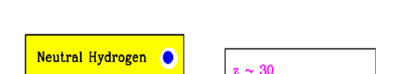
Figure 4: Stages in the reionization of hydrogen in the intergalactic medium.

Since recent observations confine the standard set of cosmological parameters to a relatively narrow range, we assume a $\Lambda$CDM cosmology with a particular standard set of parameters in the quantitative results in this review. For the contributions to the energy density, we assume ratios relative to the critical density of ${\Omega_{m}}=0.3$, ${\Omega_{\Lambda}}=0.7$, and $\Omega_{b}=0.045$, for matter, vacuum (cosmological constant), and baryons, respectively. We also assume a Hubble constant $H_{0}=100\,h\mbox{ km s}^{-1}\mbox{Mpc}^{-1}$ with $h=0.7$, and a primordial scale invariant ($n=1$) power spectrum with $\sigma_{8}=0.9$, where $\sigma_{8}$ is the root-mean-square amplitude of mass fluctuations in spheres of radius $8\ h^{-1}$ Mpc. These parameter values are based primarily on the following observational results: CMB temperature anisotropy measurements on large scales (Bennett et al. 1996) and on the scale of $\sim 1^{\circ}$ (Lange et al. 2000; Balbi et al. 2000); the abundance of galaxy clusters locally (Viana & Liddle 1999; Pen 1998; Eke, Cole, & Frenk 1996) and as a function of redshift (Bahcall & Fan 1998; Eke, Cole, Frenk, & Henry 1998); the baryon density inferred from big bang nucleosynthesis (see the review by Tytler et al. 2000); distance measurements used to derive the Hubble constant (Mould et al. 2000; Jha et al. 1999; Tonry et al. 1997; but see Theureau et al. 1997; Parodi et al. 2000); and indications of cosmic acceleration from distances based on type Ia supernovae (Perlmutter et al. 1999; Riess et al. 1998).

This review summarizes recent theoretical advances in understanding the physics of the first generation of cosmic structures. Although the literature on this subject extends all the way back to the sixties (Saslaw & Zipoy 1967, Peebles & Dicke 1968, Hirasawa 1969, Matsuda et al. 1969, Hutchins 1976, Silk 1983, Palla et al. 1983, Lepp & Shull 1984, Couchman 1985, Couchman & Rees 1986, Lahav 1986), this review focuses on the progress made over the past decade in the modern context of CDM cosmologies.

2 Hierarchical Formation of Cold Dark Matter Halos

2.1 The Expanding Universe

The modern physical description of the universe as a whole can be traced back to Einstein, who argued theoretically for the so-called “cosmological principle”: that the distribution of matter and energy must be homogeneous and isotropic on the largest scales. Today isotropy is well established (see the review by Wu, Lahav, & Rees 1999) for the distribution of faint radio sources, optically-selected galaxies, the X-ray background, and most importantly the cosmic microwave background (henceforth, CMB; see, e.g., Bennett et al. 1996). The constraints on homogeneity are less strict, but a cosmological model in which the universe is isotropic but significantly inhomogeneous in spherical shells around our special location is also excluded (Goodman 1995).

In General Relativity, the metric for a space which is spatially homogeneous and isotropic is the Robertson-Walker metric, which can be written in the form

$$ds^{2}=dt^{2}-a^{2}(t)\left[\frac{dR^{2}}{1-k\,R^{2}}+R^{2}\left(d\theta^{2}+\sin^{2}\theta\,d\phi^{2}\right)\right]\ ,$$ (2)

where $a(t)$ is the cosmic scale factor which describes expansion in time, and $(R,\theta,\phi)$ are spherical comoving coordinates. The constant $k$ determines the geometry of the metric; it is positive in a closed universe, zero in a flat universe, and negative in an open universe. Observers at rest remain at rest, at fixed $(R,\theta,\phi)$, with their physical separation increasing with time in proportion to $a(t)$. A given observer sees a nearby observer at physical distance $D$ receding at the Hubble velocity $H(t)D$, where the Hubble constant at time $t$ is $H(t)=d\ln a(t)/dt$. Light emitted by a source at time $t$ is observed at $t=0$ with a redshift $z=1/a(t)-1$, where we set $a(t=0)\equiv 1$.

The Einstein field equations of General Relativity yield the Friedmann equation (e.g., Weinberg 1972; Kolb & Turner 1990)

$$H^{2}(t)=\frac{8\pi G}{3}\rho-\frac{k}{a^{2}}\ ,$$ (3)

which relates the expansion of the universe to its matter-energy content. For each component of the energy density $\rho$, with an equation of state $p=p(\rho)$, the density $\rho$ varies with $a(t)$ according to the equation of energy conservation

$$d(\rho R^{3})=-pd(R^{3})\ .$$ (4)

With the critical density

$$\rho_{C}(t)\equiv\frac{3H^{2}(t)}{8\pi G}$$ (5)

defined as the density needed for $k=0$, we define the ratio of the total density to the critical density as

$$\Omega\equiv\frac{\rho}{\rho_{C}}\ .$$ (6)

With ${\Omega_{m}}$, ${\Omega_{\Lambda}}$, and ${\Omega_{r}}$ denoting the present contributions to $\Omega$ from matter (including cold dark matter as well as a contribution $\Omega_{b}$ from baryons), vacuum density (cosmological constant), and radiation, respectively, the Friedmann equation becomes

$$\frac{H(t)}{H_{0}}=\left[\frac{{\Omega_{m}}}{a^{3}}+{\Omega_{\Lambda}}+\frac{{\Omega_{r}}}{a^{4}}+\frac{{\Omega_{k}}}{a^{2}}\right]^{1/2}\ ,$$ (7)

where we define $H_{0}$ and $\Omega_{0}={\Omega_{m}}+{\Omega_{\Lambda}}+{\Omega_{r}}$ to be the present values of $H$ and $\Omega$, respectively, and we let

$${\Omega_{k}}\equiv-\frac{k}{H_{0}^{2}}=1-\Omega_{0}.$$ (8)

In the particularly simple Einstein-de Sitter model (${\Omega_{m}}=1$, ${\Omega_{\Lambda}}={\Omega_{r}}={\Omega_{k}}=0$), the scale factor varies as $a(t)\propto t^{2/3}$. Even models with non-zero ${\Omega_{\Lambda}}$ or ${\Omega_{k}}$ approach the Einstein-de Sitter behavior at high redshifts, i.e., when

$$(1+z)\gg{\rm max}\left[(1-\Omega_{m}-\Omega_{\Lambda})/\Omega_{m},(\Omega_{\Lambda}/\Omega_{m})^{1/3}\right]$$ (9)

(as long as ${\Omega_{r}}$ can be neglected). The Friedmann equation implies that models with ${\Omega_{k}}=0$ converge to the Einstein-de Sitter limit faster than do open models. E.g., for $\Omega_{m}=0.3$ and $\Omega_{\Lambda}=0.7$ equation (9) corresponds to the condition $z\gg 1.3$, which is easily satisfied by the reionization redshift. In this high-$z$ regime, $H(t)\approx 2/(3t)$, and the age of the universe is

$$t\approx{2\over 3\,H_{0}\sqrt{\Omega_{m}}}\left(1+z\right)^{-3/2}=5.38\times 10^{8}\left(\frac{1+z}{10}\right)^{-3/2}{\rm yr}\ ,$$ (10)

where in the last expression we assumed our standard cosmological parameters (see the end of §1).

In the standard hot Big Bang model, the universe is initially hot and the energy density is dominated by radiation. The transition to matter domination occurs at $z\sim 10^{4}$, but the universe remains hot enough that the gas is ionized, and electron-photon scattering effectively couples the matter and radiation. At $z\sim 1200$ the temperature drops below $\sim 3300$ K and protons and electrons recombine to form neutral hydrogen. The photons then decouple and travel freely until the present, when they are observed as the CMB.

2.2 Linear Gravitational Growth

Observations of the CMB (e.g., Bennett et al. 1996) show that the universe at recombination was extremely uniform, but with spatial fluctuations in the energy density and gravitational potential of roughly one part in $10^{5}$. Such small fluctuations, generated in the early universe, grow over time due to gravitational instability, and eventually lead to the formation of galaxies and the large-scale structure observed in the present universe.

As in the previous section, we distinguish between fixed and comoving coordinates. Using vector notation, the fixed coordinate ${\bf r}$ corresponds to a comoving position ${\bf x}={\bf r}/a$. In a homogeneous universe with density $\rho$, we describe the cosmological expansion in terms of an ideal pressure-less fluid of particles each of which is at fixed ${\bf x}$, expanding with the Hubble flow ${\bf v}=H(t){\bf r}$ where ${\bf v}=d{\bf r}/dt$. Onto this uniform expansion we impose small perturbations, given by a relative density perturbation

$$\delta({\bf x})=\frac{\rho({\bf r})}{\bar{\rho}}-1\ ,$$ (11)

where the mean fluid density is $\bar{\rho}$, with a corresponding peculiar velocity ${\bf u}\equiv{\bf v}-H{\bf r}$. Then the fluid is described by the continuity and Euler equations in comoving coordinates (Peebles 1980, 1993):

$$\frac{\partial\delta}{\partial t}+\frac{1}{a}{\bf\nabla}\cdot\left[(1+\delta){\bf u}\right] = 0$$ (12)

$$\frac{\partial{\bf u}}{\partial t}+H{\bf u}+\frac{1}{a}({\bf u}\cdot{\bf\nabla}){\bf u} = -\frac{1}{a}{\bf\nabla}\phi\ .$$ (13)

The potential $\phi$ is given by the Poisson equation, in terms of the density perturbation:

$$\nabla^{2}\phi=4\pi G\bar{\rho}a^{2}\delta\ .$$ (14)

This fluid description is valid for describing the evolution of collisionless cold dark matter particles until different particle streams cross. This “shell-crossing” typically occurs only after perturbations have grown to become non-linear, and at that point the individual particle trajectories must in general be followed. Similarly, baryons can be described as a pressure-less fluid as long as their temperature is negligibly small, but non-linear collapse leads to the formation of shocks in the gas.

For small perturbations $\delta\ll 1$, the fluid equations can be linearized and combined to yield

$$\frac{\partial^{2}\delta}{\partial t^{2}}+2H\frac{\partial\delta}{\partial t}=4\pi G\bar{\rho}\delta\ .$$ (15)

This linear equation has in general two independent solutions, only one of which grows with time. Starting with random initial conditions, this “growing mode” comes to dominate the density evolution. Thus, until it becomes non-linear, the density perturbation maintains its shape in comoving coordinates and grows in proportion to a growth factor $D(t)$. The growth factor is in general given by (Peebles 1980)

$$D(t)\propto\frac{\left({\Omega_{\Lambda}}a^{3}+{\Omega_{k}}a+{\Omega_{m}}\right)^{1/2}}{a^{3/2}}\int^{a}\frac{a^{3/2}\,da}{\left({\Omega_{\Lambda}}a^{3}+{\Omega_{k}}a+{\Omega_{m}}\right)^{3/2}}\ ,$$ (16)

where we neglect ${\Omega_{r}}$ when considering halos forming at $z\ll 10^{4}$. In the Einstein-de Sitter model (or, at high redshift, in other models as well) the growth factor is simply proportional to $a(t)$.

The spatial form of the initial density fluctuations can be described in Fourier space, in terms of Fourier components

$$\delta_{\bf k}=\int d^{3}x\,\delta({\bf x})e^{-i{\bf k}\cdot{\bf x}}\ .$$ (17)

Here we use the comoving wavevector ${\bf k}$, whose magnitude $k$ is the comoving wavenumber which is equal to $2\pi$ divided by the wavelength. The Fourier description is particularly simple for fluctuations generated by inflation (e.g., Kolb & Turner 1990). Inflation generates perturbations given by a Gaussian random field, in which different ${\bf k}$-modes are statistically independent, each with a random phase. The statistical properties of the fluctuations are determined by the variance of the different ${\bf k}$-modes, and the variance is described in terms of the power spectrum $P(k)$ as follows:

$$\left<\delta_{{\bf k}}\delta_{{\bf k^{\prime}}}^{*}\right>=\left(2\pi\right)^{3}P(k)\,\delta^{(3)}\left({\bf k}-{\bf k^{\prime}}\right)\ ,$$ (18)

where $\delta^{(3)}$ is the three-dimensional Dirac delta function.

In standard models, inflation produces a primordial power-law spectrum $P(k)\propto k^{n}$ with $n\sim 1$. Perturbation growth in the radiation-dominated and then matter-dominated universe results in a modified final power spectrum, characterized by a turnover at a scale of order the horizon $cH^{-1}$ at matter-radiation equality, and a small-scale asymptotic shape of $P(k)\propto k^{n-4}$. On large scales the power spectrum evolves in proportion to the square of the growth factor, and this simple evolution is termed linear evolution. On small scales, the power spectrum changes shape due to the additional non-linear gravitational growth of perturbations, yielding the full, non-linear power spectrum. The overall amplitude of the power spectrum is not specified by current models of inflation, and it is usually set observationally using the CMB temperature fluctuations or local measures of large-scale structure.

Since density fluctuations may exist on all scales, in order to determine the formation of objects of a given size or mass it is useful to consider the statistical distribution of the smoothed density field. Using a window function $W({\bf y})$ normalized so that $\int d^{3}{\bf y}\,W({\bf y})=1$, the smoothed density perturbation field, $\int d^{3}{\bf y}\delta({\bf x}+{\bf y})W({\bf y})$, itself follows a Gaussian distribution with zero mean. For the particular choice of a spherical top-hat, in which $W=1$ in a sphere of radius $R$ and is zero outside, the smoothed perturbation field measures the fluctuations in the mass in spheres of radius $R$. The normalization of the present power spectrum is often specified by the value of $\sigma_{8}\equiv\sigma(R=8h^{-1}{\rm Mpc})$. For the top-hat, the smoothed perturbation field is denoted $\delta_{R}$ or $\delta_{M}$, where the mass $M$ is related to the comoving radius $R$ by $M=4\pi\rho_{m}R^{3}/3$, in terms of the current mean density of matter $\rho_{m}$. The variance $\langle\delta_{M}\rangle^{2}$ is

$$\sigma^{2}(M)=\sigma^{2}(R)=\int_{0}^{\infty}\frac{dk}{2\pi^{2}}\,k^{2}P(k)\left[\frac{3j_{1}(kR)}{kR}\right]^{2}\ ,$$ (19)

where $j_{1}(x)=(\sin x-x\cos x)/x^{2}$. The function $\sigma(M)$ plays a crucial role in estimates of the abundance of collapsed objects, as described below.

2.3 Formation of Nonlinear Objects

The small density fluctuations evidenced in the CMB grow over time as described in the previous subsection, until the perturbation $\delta$ becomes of order unity, and the full non-linear gravitational problem must be considered. The dynamical collapse of a dark matter halo can be solved analytically only in cases of particular symmetry. If we consider a region which is much smaller than the horizon $cH^{-1}$, then the formation of a halo can be formulated as a problem in Newtonian gravity, in some cases with minor corrections coming from General Relativity. The simplest case is that of spherical symmetry, with an initial ($t=t_{i}\ll t_{0}$) top-hat of uniform overdensity $\delta_{i}$ inside a sphere of radius $R$. Although this model is restricted in its direct applicability, the results of spherical collapse have turned out to be surprisingly useful in understanding the properties and distribution of halos in models based on cold dark matter.

The collapse of a spherical top-hat is described by the Newtonian equation (with a correction for the cosmological constant)

$$\frac{d^{2}r}{dt^{2}}=H_{0}^{2}{\Omega_{\Lambda}}\,r-\frac{GM}{r^{2}}\ ,$$ (20)

where $r$ is the radius in a fixed (not comoving) coordinate frame, $H_{0}$ is the present Hubble constant, $M$ is the total mass enclosed within radius $r$, and the initial velocity field is given by the Hubble flow $dr/dt=H(t)r$. The enclosed $\delta$ grows initially as $\delta_{L}=\delta_{i}D(t)/D(t_{i})$, in accordance with linear theory, but eventually $\delta$ grows above $\delta_{L}$. If the mass shell at radius $r$ is bound (i.e., if its total Newtonian energy is negative) then it reaches a radius of maximum expansion and subsequently collapses. At the moment when the top-hat collapses to a point, the overdensity predicted by linear theory is (Peebles 1980) $\delta_{L}\,=1.686$ in the Einstein-de Sitter model, with only a weak dependence on ${\Omega_{m}}$ and ${\Omega_{\Lambda}}$. Thus a top-hat collapses at redshift $z$ if its linear overdensity extrapolated to the present day (also termed the critical density of collapse) is

$$\delta_{\rm crit}(z)=\frac{1.686}{D(z)}\ ,$$ (21)

where we set $D(z=0)=1$.

Even a slight violation of the exact symmetry of the initial perturbation can prevent the top-hat from collapsing to a point. Instead, the halo reaches a state of virial equilibrium by violent relaxation (phase mixing). Using the virial theorem $U=-2K$ to relate the potential energy $U$ to the kinetic energy $K$ in the final state, the final overdensity relative to the critical density at the collapse redshift is $\Delta_{c}=18\pi^{2}\simeq 178$ in the Einstein-de Sitter model, modified in a universe with ${\Omega_{m}}+{\Omega_{\Lambda}}=1$ to the fitting formula (Bryan & Norman 1998)

$$\Delta_{c}=18\pi^{2}+82d-39d^{2}\ ,$$ (22)

where $d\equiv{\Omega_{m}^{\,z}}-1$ is evaluated at the collapse redshift, so that

$${\Omega_{m}^{\,z}}=\frac{{\Omega_{m}}(1+z)^{3}}{{\Omega_{m}}(1+z)^{3}+{\Omega_{\Lambda}}+{\Omega_{k}}(1+z)^{2}}\ .$$ (23)

A halo of mass $M$ collapsing at redshift $z$ thus has a (physical) virial radius

$$r_{\rm vir}=0.784\left(\frac{M}{10^{8}\ h^{-1}\ M_{\sun}}\right)^{1/3}\left[\frac{{\Omega_{m}}}{{\Omega_{m}^{\,z}}}\ \frac{\Delta_{c}}{18\pi^{2}}\right]^{-1/3}\left(\frac{1+z}{10}\right)^{-1}\ h^{-1}\ {\rm kpc}\ ,$$ (24)

and a corresponding circular velocity,

$$V_{c}=\left(\frac{GM}{r_{\rm vir}}\right)^{1/2}=23.4\left(\frac{M}{10^{8}\ h^{-1}\ M_{\sun}}\right)^{1/3}\left[\frac{{\Omega_{m}}}{{\Omega_{m}^{\,z}}}\ \frac{\Delta_{c}}{18\pi^{2}}\right]^{1/6}\left(\frac{1+z}{10}\right)^{1/2}\ {\rm km\ s}^{-1}\ .$$ (25)

In these expressions we have assumed a present Hubble constant written in the form $H_{0}=100\,h\mbox{ km s}^{-1}\mbox{Mpc}^{-1}$. We may also define a virial temperature

$$T_{\rm vir}=\frac{\mu m_{p}V_{c}^{2}}{2k_{\rm B}}=1.98\times 10^{4}\ \left(\frac{\mu}{0.6}\right)\left(\frac{M}{10^{8}\ h^{-1}\ M_{\sun}}\right)^{2/3}\left[\frac{{\Omega_{m}}}{{\Omega_{m}^{\,z}}}\ \frac{\Delta_{c}}{18\pi^{2}}\right]^{1/3}\left(\frac{1+z}{10}\right)\ {\rm K}\ ,$$ (26)

where $\mu$ is the mean molecular weight and $m_{p}$ is the proton mass. Note that the value of $\mu$ depends on the ionization fraction of the gas; $\mu=0.59$ for a fully ionized primordial gas, $\mu=0.61$ for a gas with ionized hydrogen but only singly-ionized helium, and $\mu=1.22$ for neutral primordial gas. The binding energy of the halo is approximately

$$E_{b}={1\over 2}\frac{GM^{2}}{r_{\rm vir}}=5.45\times 10^{53}\left(\frac{M}{10^{8}\ h^{-1}\ M_{\sun}}\right)^{5/3}\left[\frac{{\Omega_{m}}}{{\Omega_{m}^{\,z}}}\ \frac{\Delta_{c}}{18\pi^{2}}\right]^{1/3}\left(\frac{1+z}{10}\right)h^{-1}\ {\rm erg}\ .$$ (27)

Note that the binding energy of the baryons is smaller by a factor equal to the baryon fraction $\Omega_{b}/{\Omega_{m}}$.

Although spherical collapse captures some of the physics governing the formation of halos, structure formation in cold dark matter models proceeds hierarchically. At early times, most of the dark matter is in low-mass halos, and these halos continuously accrete and merge to form high-mass halos. Numerical simulations of hierarchical halo formation indicate a roughly universal spherically-averaged density profile for the resulting halos (Navarro, Frenk, & White 1997, hereafter NFW), though with considerable scatter among different halos (e.g., Bullock et al. 2000). The NFW profile has the form

$$\rho(r)=\frac{3H_{0}^{2}}{8\pi G}(1+z)^{3}\frac{{\Omega_{m}}}{{\Omega_{m}^{\,z}}}\frac{\delta_{c}}{c_{\rm N}x(1+c_{\rm N}x)^{2}}\ ,$$ (28)

where $x=r/r_{\rm vir}$, and the characteristic density $\delta_{c}$ is related to the concentration parameter $c_{\rm N}$ by

$$\delta_{c}=\frac{\Delta_{c}}{3}\frac{c_{\rm N}^{3}}{\ln(1+c_{\rm N})-c_{\rm N}/(1+c_{\rm N})}\ .$$ (29)

The concentration parameter itself depends on the halo mass $M$, at a given redshift $z$. We note that the dense, cuspy halo profile predicted by CDM models is not apparent in the mass distribution derived from measurements of the rotation curves of dwarf galaxies (e.g., de Blok & McGaugh 1997; Salucci & Burkert 2000), although observational and modeling uncertainties may preclude a firm conclusion at present (van den Bosch et al. 2000; Swaters, Madore, & Trewhella 2000).

2.4 The Abundance of Dark Matter Halos

In addition to characterizing the properties of individual halos, a critical prediction of any theory of structure formation is the abundance of halos, i.e., the number density of halos as a function of mass, at any redshift. This prediction is an important step toward inferring the abundances of galaxies and galaxy clusters. While the number density of halos can be measured for particular cosmologies in numerical simulations, an analytic model helps us gain physical understanding and can be used to explore the dependence of abundances on all the cosmological parameters.

A simple analytic model which successfully matches most of the numerical simulations was developed by Press & Schechter (1974). The model is based on the ideas of a Gaussian random field of density perturbations, linear gravitational growth, and spherical collapse. To determine the abundance of halos at a redshift $z$, we use $\delta_{M}$, the density field smoothed on a mass scale $M$, as defined in §2.2. Although the model is based on the initial conditions, it is usually expressed in terms of redshift-zero quantities. Thus, we use the linearly-extrapolated density field, i.e., the initial density field at high redshift extrapolated to the present by simple multiplication by the relative growth factor (see §2.2). Similarly, in this section the ’present power spectrum’ refers to the initial power spectrum, linearly-extrapolated to the present without including non-linear evolution. Since $\delta_{M}$ is distributed as a Gaussian variable with zero mean and standard deviation $\sigma(M)$ [which depends only on the present power spectrum, see equation (19)], the probability that $\delta_{M}$ is greater than some $\delta$ equals

$$\int_{\delta}^{\infty}d\delta_{M}\frac{1}{\sqrt{2\pi}\,\sigma(M)}\exp\left[-\frac{\delta_{M}^{2}}{2\,\sigma^{2}(M)}\right]={1\over 2}{\rm erfc}\left(\frac{\delta}{\sqrt{2}\,\sigma}\right)\ .$$ (30)

The fundamental ansatz is to identify this probability with the fraction of dark matter particles which are part of collapsed halos of mass greater than $M$, at redshift $z$. There are two additional ingredients: First, the value used for $\delta$ is $\delta_{\rm crit}(z)$ given in equation (21), which is the critical density of collapse found for a spherical top-hat (extrapolated to the present since $\sigma(M)$ is calculated using the present power spectrum); and second, the fraction of dark matter in halos above $M$ is multiplied by an additional factor of 2 in order to ensure that every particle ends up as part of some halo with $M>0$. Thus, the final formula for the mass fraction in halos above $M$ at redshift $z$ is

$$F(>M|z)={\rm erfc}\left(\frac{\delta_{\rm crit}(z)}{\sqrt{2}\,\sigma}\right)\ .$$ (31)

This ad-hoc factor of 2 is necessary, since otherwise only positive fluctuations of $\delta_{M}$ would be included. Bond et al. (1991) found an alternate derivation of this correction factor, using a different ansatz. In their derivation, the factor of 2 has a more satisfactory origin, namely the so-called “cloud-in-cloud” problem: For a given mass $M$, even if $\delta_{M}$ is smaller than $\delta_{\rm crit}(z)$, it is possible that the corresponding region lies inside a region of some larger mass $M_{L}>M$, with $\delta_{M_{L}}>\delta_{\rm crit}(z)$. In this case the original region should be counted as belonging to a halo of mass $M_{L}$. Thus, the fraction of particles which are part of collapsed halos of mass greater than $M$ is larger than the expression given in equation (30). Bond et al. showed that, under certain assumptions, the additional contribution results precisely in a factor of 2 correction.

Differentiating the fraction of dark matter in halos above $M$ yields the mass distribution. Letting $dn$ be the comoving number density of halos of mass between $M$ and $M+dM$, we have

$$\frac{dn}{dM}=\sqrt{\frac{2}{\pi}}\,\frac{\rho_{m}}{M}\,\frac{-d(\ln\sigma)}{dM}\,\nu_{c}\,e^{-\nu_{c}^{2}/2}\ ,$$ (32)

where $\nu_{c}=\delta_{\rm crit}(z)/\sigma(M)$ is the number of standard deviations which the critical collapse overdensity represents on mass scale $M$. Thus, the abundance of halos depends on the two functions $\sigma(M)$ and $\delta_{\rm crit}(z)$, each of which depends on the energy content of the universe and the values of the other cosmological parameters. We illustrate the abundance of halos for our standard choice of the $\Lambda$CDM model with ${\Omega_{m}}=0.3$ (see the end of §1).

Figure 5 shows $\sigma(M)$ and $\delta_{\rm crit}(z)$, with the input power spectrum computed from Eisenstein & Hu (1999). The solid line is $\sigma(M)$ for the cold dark matter model with the parameters specified above. The horizontal dotted lines show the value of $\delta_{\rm crit}(z)$ at $z=0,2,5,10,20$ and 30, as indicated in the figure. From the intersection of these horizontal lines with the solid line we infer, e.g., that at $z=5$ a $1-\sigma$ fluctuation on a mass scale of $2\times 10^{7}M_{\sun}$ will collapse. On the other hand, at $z=5$ collapsing halos require a $2-\sigma$ fluctuation on a mass scale of $3\times 10^{10}M_{\sun}$, since $\sigma(M)$ on this mass scale equals about half of $\delta_{\rm crit}(z=5)$. Since at each redshift a fixed fraction ($31.7\%$) of the total dark matter mass lies in halos above the $1-\sigma$ mass, Figure 5 shows that most of the mass is in small halos at high redshift, but it continuously shifts toward higher characteristic halo masses at lower redshift. Note also that $\sigma(M)$ flattens at low masses because of the changing shape of the power spectrum. Since $\sigma\rightarrow\infty$ as $M\rightarrow 0$, in the cold dark matter model all the dark matter is tied up in halos at all redshifts, if sufficiently low-mass halos are considered.

Also shown in Figure 5 is the effect of cutting off the power spectrum on small scales. The short-dashed curve corresponds to the case where the power spectrum is set to zero above a comoving wavenumber $k=10\,{\rm Mpc}^{-1}$, which corresponds to a mass $M=1.7\times 10^{8}M_{\sun}$. The long-dashed curve corresponds to a more radical cutoff above $k=1\,{\rm Mpc}^{-1}$, or below $M=1.7\times 10^{11}M_{\sun}$. A cutoff severely reduces the abundance of low-mass halos, and the finite value of $\sigma(M=0)$ implies that at all redshifts some fraction of the dark matter does not fall into halos. At high redshifts where $\delta_{\rm crit}(z)\gg\sigma(M=0)$, all halos are rare and only a small fraction of the dark matter lies in halos. In particular, this can affect the abundance of halos at the time of reionization, and thus the observed limits on reionization constrain scenarios which include a small-scale cutoff in the power spectrum (Barkana, Haiman, & Ostriker 2000).

In Figures 6 – 9 we show explicitly the properties of collapsing halos which represent $1-\sigma$, $2-\sigma$, and $3-\sigma$ fluctuations (corresponding in all cases to the curves in order from bottom to top), as a function of redshift. No cutoff is applied to the power spectrum. Figure 6 shows the halo mass, Figure 7 the virial radius, Figure 8 the virial temperature (with $\mu$ in equation (26) set equal to $0.6$, although low temperature halos contain neutral gas) as well as circular velocity, and Figure 9 shows the total binding energy of these halos. In Figures 6 and 8, the dashed curves indicate the minimum virial temperature required for efficient cooling (see §3.3) with primordial atomic species only (upper curve) or with the addition of molecular hydrogen (lower curve). Figure 9 shows the binding energy of dark matter halos. The binding energy of the baryons is a factor $\sim\Omega_{b}/\Omega_{m}\sim 15\%$ smaller, if they follow the dark matter. Except for this constant factor, the figure shows the minimum amount of energy that needs to be deposited into the gas in order to unbind it from the potential well of the dark matter. For example, the hydrodynamic energy released by a single supernovae, $\sim 10^{51}~{}{\rm erg}$, is sufficient to unbind the gas in all $1-\sigma$ halos at $z\gtrsim 5$ and in all $2-\sigma$ halos at $z\gtrsim 12$.

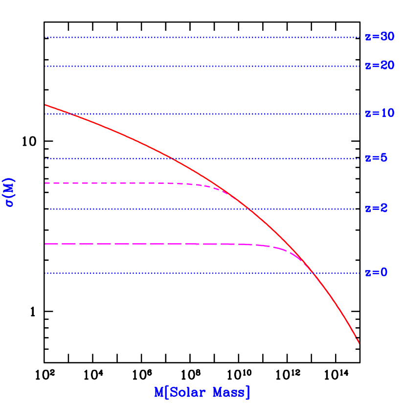
Figure 5: Mass fluctuations and collapse thresholds in cold dark matter models. The horizontal dotted lines show the value of the extrapolated collapse overdensity $\delta_{\rm crit}(z)$ at the indicated redshifts. Also shown is the value of $\sigma(M)$ for the cosmological parameters given in the text (solid curve), as well as $\sigma(M)$ for a power spectrum with a cutoff below a mass $M=1.7\times 10^{8}M_{\sun}$ (short-dashed curve), or $M=1.7\times 10^{11}M_{\sun}$ (long-dashed curve). The intersection of the horizontal lines with the other curves indicate, at each redshift $z$, the mass scale (for each model) at which a $1-\sigma$ fluctuation is just collapsing at $z$ (see the discussion in the text).

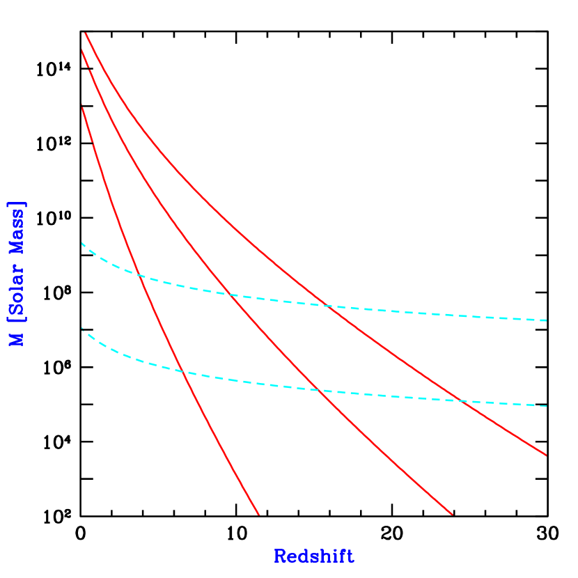
Figure 6: Characteristic properties of collapsing halos: Halo mass. The solid curves show the mass of collapsing halos which correspond to $1-\sigma$, $2-\sigma$, and $3-\sigma$ fluctuations (in order from bottom to top). The dashed curves show the mass corresponding to the minimum temperature required for efficient cooling with primordial atomic species only (upper curve) or with the addition of molecular hydrogen (lower curve).

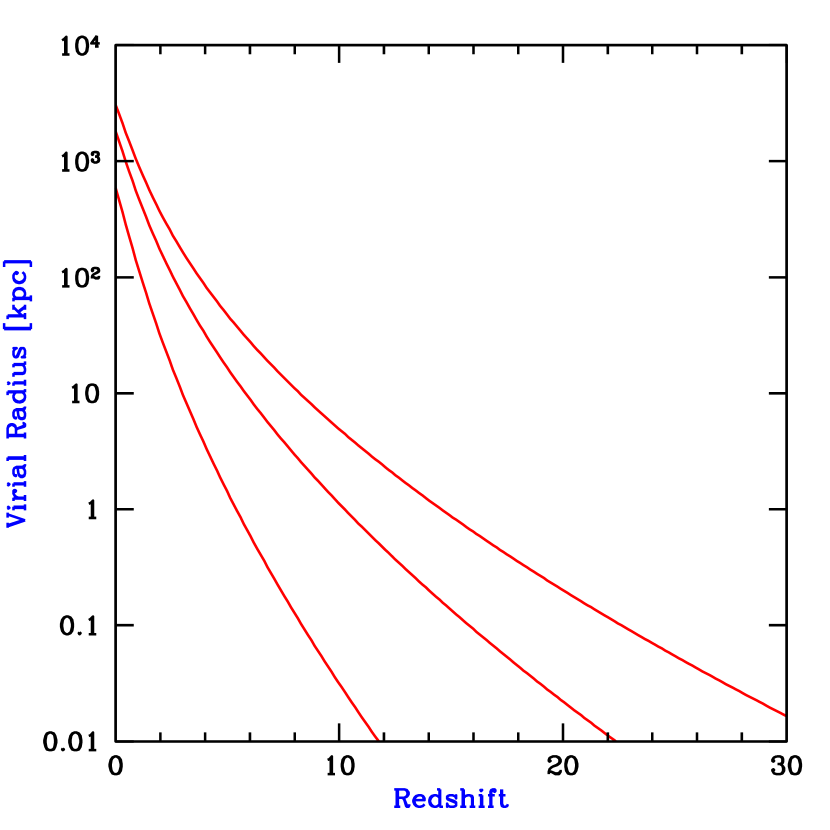
Figure 7: Characteristic properties of collapsing halos: Halo virial radius. The curves show the virial radius of collapsing halos which correspond to $1-\sigma$, $2-\sigma$, and $3-\sigma$ fluctuations (in order from bottom to top).

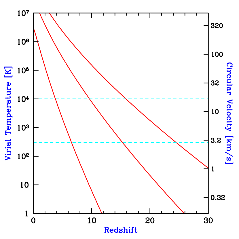
Figure 8: Characteristic properties of collapsing halos: Halo virial temperature and circular velocity. The solid curves show the virial temperature (or, equivalently, the circular velocity) of collapsing halos which correspond to $1-\sigma$, $2-\sigma$, and $3-\sigma$ fluctuations (in order from bottom to top). The dashed curves show the minimum temperature required for efficient cooling with primordial atomic species only (upper curve) or with the addition of molecular hydrogen (lower curve).

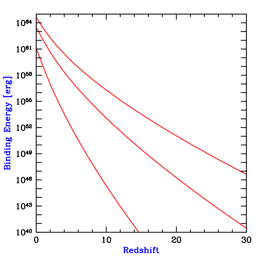
Figure 9: Characteristic properties of collapsing halos: Halo binding energy. The curves show the total binding energy of collapsing halos which correspond to $1-\sigma$, $2-\sigma$, and $3-\sigma$ fluctuations (in order from bottom to top).

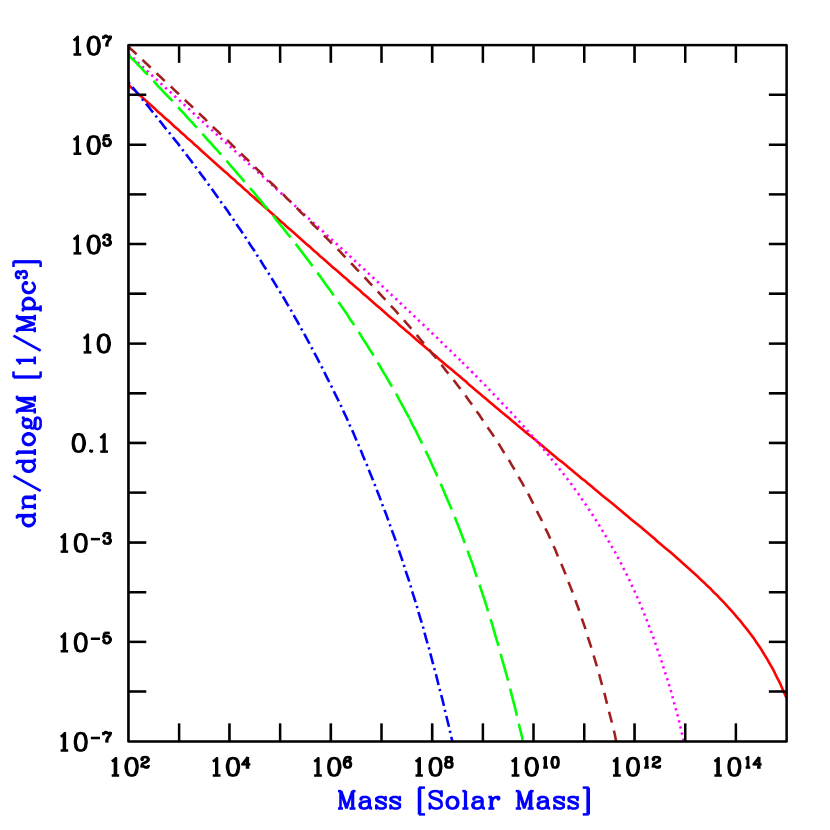
Figure 10: Halo mass function at several redshifts: $z=0$ (solid curve), $z=5$ (dotted curve), $z=10$ (short-dashed curve), $z=20$ (long-dashed curve), and $z=30$ (dot-dashed curve).

At $z=5$, the halo masses which correspond to $1-\sigma$, $2-\sigma$, and $3-\sigma$ fluctuations are $1.8\times 10^{7}M_{\sun}$, $3.0\times 10^{10}M_{\sun}$, and $7.0\times 10^{11}M_{\sun}$, respectively. The corresponding virial temperatures are $2.0\times 10^{3}$ K, $2.8\times 10^{5}$ K, and $2.3\times 10^{6}$ K. The equivalent circular velocities are 7.5 ${\rm km\ s}^{-1}$, 88 ${\rm km\ s}^{-1}$, and 250 ${\rm km\ s}^{-1}$. At $z=10$, the $1-\sigma$, $2-\sigma$, and $3-\sigma$ fluctuations correspond to halo masses of $1.3\times 10^{3}M_{\sun}$, $5.7\times 10^{7}M_{\sun}$, and $4.8\times 10^{9}M_{\sun}$, respectively. The corresponding virial temperatures are 6.2 K, $7.9\times 10^{3}$ K, and $1.5\times 10^{5}$ K. The equivalent circular velocities are 0.41 ${\rm km\ s}^{-1}$, 15 ${\rm km\ s}^{-1}$, and 65 ${\rm km\ s}^{-1}$. Atomic cooling is efficient at $T_{\rm vir}\gtrsim 10^{4}$ K, or a circular velocity $V_{c}\gtrsim 17\ {\rm km\ s}^{-1}$. This corresponds to a $1.2-\sigma$ fluctuation and a halo mass of $2.1\times 10^{8}M_{\sun}$ at $z=5$, and a $2.1-\sigma$ fluctuation and a halo mass of $8.3\times 10^{7}M_{\sun}$ at $z=10$. Molecular hydrogen provides efficient cooling down to $T_{\rm vir}\sim 300$ K, or a circular velocity $V_{c}\sim 2.0\ {\rm km\ s}^{-1}$. This corresponds to a $0.76-\sigma$ fluctuation and a halo mass of $3.5\times 10^{5}M_{\sun}$ at $z=5$, and a $1.3-\sigma$ fluctuation and a halo mass of $1.4\times 10^{5}M_{\sun}$ at $z=10$.

In Figure 10 we show the halo mass function $dn/d\ln(M)$ at several different redshifts: $z=0$ (solid curve), $z=5$ (dotted curve), $z=10$ (short-dashed curve), $z=20$ (long-dashed curve), and $z=30$ (dot-dashed curve). Note that the mass function does not decrease monotonically with redshift at all masses. At the lowest masses, the abundance of halos is higher at $z>0$ than at $z=0$.

3 Gas Infall and Cooling in Dark Matter Halos

3.1 Cosmological Jeans Mass

The Jeans length $\lambda_{\rm J}$ was originally defined (Jeans 1928) in Newtonian gravity as the critical wavelength that separates oscillatory and exponentially-growing density perturbations in an infinite, uniform, and stationary distribution of gas. On scales $\ell$ smaller than $\lambda_{\rm J}$, the sound crossing time, $\ell/c_{s}$ is shorter than the gravitational free-fall time, $(G\rho)^{-1/2}$, allowing the build-up of a pressure force that counteracts gravity. On larger scales, the pressure gradient force is too slow to react to a build-up of the attractive gravitational force. The Jeans mass is defined as the mass within a sphere of radius $\lambda_{\rm J}/2$, $M_{\rm J}=(4\pi/3)\rho(\lambda_{\rm J}/2)^{3}$. In a perturbation with a mass greater than $M_{\rm J}$, the self-gravity cannot be supported by the pressure gradient, and so the gas is unstable to gravitational collapse. The Newtonian derivation of the Jeans instability suffers from a conceptual inconsistency, as the unperturbed gravitational force of the uniform background must induce bulk motions (compare Binney & Tremaine 1987). However, this inconsistency is remedied when the analysis is done in an expanding universe.

The perturbative derivation of the Jeans instability criterion can be carried out in a cosmological setting by considering a sinusoidal perturbation superposed on a uniformly expanding background. Here, as in the Newtonian limit, there is a critical wavelength $\lambda_{\rm J}$ that separates oscillatory and growing modes. Although the expansion of the background slows down the exponential growth of the amplitude to a power-law growth, the fundamental concept of a minimum mass that can collapse at any given time remains the same (see, e.g. Kolb & Turner 1990; Peebles 1993).

We consider a mixture of dark matter and baryons with density parameters $\Omega_{\rm dm}^{\,z}=\bar{\rho}_{\rm dm}/\rho_{\rm c}$ and $\Omega_{\rm b}^{\,z}=\bar{\rho}_{\rm b}/\rho_{\rm c}$, where $\bar{\rho}_{\rm dm}$ is the average dark matter density, $\bar{\rho}_{\rm b}$ is the average baryonic density, $\rho_{\rm c}$ is the critical density, and $\Omega_{\rm dm}^{\,z}+\Omega_{\rm b}^{\,z}={\Omega_{m}^{\,z}}$ is given by equation (23). We also assume spatial fluctuations in the gas and dark matter densities with the form of a single spherical Fourier mode on a scale much smaller than the horizon,

$$\frac{\rho_{\rm dm}(r,t)-\bar{\rho}_{\rm dm}(t)}{\bar{\rho}_{\rm dm}(t)} = \delta_{\rm dm}(t)\frac{\sin(kr)}{kr}\ ,$$ (33)

$$\frac{\rho_{\rm b}(r,t)-\bar{\rho}_{\rm b}(t)}{\bar{\rho}_{\rm b}(t)} = \delta_{\rm b}(t)\frac{\sin(kr)}{kr}\ ,$$ (34)

where $\bar{\rho}_{\rm dm}(t)$ and $\bar{\rho}_{\rm b}(t)$ are the background densities of the dark matter and baryons, $\delta_{\rm dm}(t)$ and $\delta_{\rm b}(t)$ are the dark matter and baryon overdensity amplitudes, $r$ is the comoving radial coordinate, and $k$ is the comoving perturbation wavenumber. We adopt an ideal gas equation-of-state for the baryons with a specific heat ratio $\gamma$=$5/3$. Initially, at time $t=t_{\rm i}$, the gas temperature is uniform $T_{\rm b}(r,t_{\rm i})$=$T_{\rm i}$, and the perturbation amplitudes are small $\delta_{\rm dm,i},\delta_{\rm b,i}\ll 1$. We define the region inside the first zero of $\sin(kr)/(kr)$, namely $0<kr<\pi$, as the collapsing “object”.

The evolution of the temperature of the baryons $T_{\rm b}(r,t)$ in the linear regime is determined by the coupling of their free electrons to the Cosmic Microwave Background (CMB) through Compton scattering, and by the adiabatic expansion of the gas. Hence, $T_{\rm b}(r,t)$ is generally somewhere between the CMB temperature, $T_{\gamma}\propto(1+z)^{-1}$ and the adiabatically-scaled temperature $T_{\rm ad}\propto(1+z)^{-2}$. In the limit of tight coupling to $T_{\gamma}$, the gas temperature remains uniform. On the other hand, in the adiabatic limit, the temperature develops a gradient according to the relation

$$T_{\rm b}\propto\rho_{b}^{(\gamma-1)}.$$ (35)

The evolution of dark matter overdensity, $\delta_{\rm dm}(t)$, in the linear regime is described by the equation (see §9.3.2 of Kolb & Turner 1990),

$${\ddot{\delta}}_{\rm dm}+2H{\dot{\delta}}_{\rm dm}={3\over 2}H^{2}\left(\Omega_{\rm b}\delta_{\rm b}+\Omega_{\rm dm}\delta_{\rm dm}\right)$$ (36)

whereas the evolution of the overdensity of the baryons, $\delta_{\rm b}(t)$, is described by

$${\ddot{\delta}}_{\rm b}+2H{\dot{\delta}}_{\rm b}={3\over 2}H^{2}\left(\Omega_{\rm b}\delta_{\rm b}+\Omega_{\rm dm}\delta_{\rm dm}\right)-\frac{k_{\rm B}T_{\rm i}}{\mu m_{p}}\left({k\over a}\right)^{2}\left(\frac{a_{\rm i}}{a}\right)^{(1+\beta)}\left(\delta_{\rm b}+{2\over 3}\beta[\delta_{\rm b}-\delta_{\rm b,i}]\right).$$ (37)

Here, $H(t)={\dot{a}}/a$ is the Hubble parameter at a cosmological time $t$, and $\mu=1.22$ is the mean molecular weight of the neutral primordial gas in atomic units. The parameter $\beta$ distinguishes between the two limits for the evolution of the gas temperature. In the adiabatic limit $\beta=1$, and when the baryon temperature is uniform and locked to the background radiation, $\beta=0$. The last term on the right hand side (in square brackets) takes into account the extra pressure gradient force in $\nabla(\rho_{\rm b}T)=(T\nabla\rho_{\rm b}+\rho_{\rm b}\nabla T)$, arising from the temperature gradient which develops in the adiabatic limit. The Jeans wavelength $\lambda_{\rm J}=2\pi/k_{\rm J}$ is obtained by setting the right-hand side of equation (37) to zero, and solving for the critical wavenumber $k_{\rm J}$. As can be seen from equation (37), the critical wavelength $\lambda_{\rm J}$ (and therefore the mass $M_{\rm J}$) is in general time-dependent. We infer from equation (37) that as time proceeds, perturbations with increasingly smaller initial wavelengths stop oscillating and start to grow.

To estimate the Jeans wavelength, we equate the right-hand-side of equation (37) to zero. We further approximate $\delta_{\rm b}\sim\delta_{\rm dm}$, and consider sufficiently high redshifts at which the universe is matter-dominated and flat (equations (9) and (10) in §2.1). We also assume $\Omega_{\rm b}\ll{\Omega_{m}}$, where $\Omega_{m}=\Omega_{\rm dm}+\Omega_{b}$ is the total matter density parameter. Following cosmological recombination at $z\approx 10^{3}$, the residual ionization of the cosmic gas keeps its temperature locked to the CMB temperature (via Compton scattering) down to a redshift of (p. 179 of Peebles 1993)

$$1+z_{t}\approx 137(\Omega_{b}h^{2}/0.022)^{2/5}\ .$$ (38)

In the redshift range between recombination and $z_{t}$, $\beta=0$ and

$$k_{\rm J}\equiv(2\pi/\lambda_{\rm J})=[2k_{\rm B}T_{\gamma}(0)/3\mu m_{p}]^{-1/2}{\sqrt{\Omega_{m}}}H_{0}\ ,$$ (39)

so that the Jeans mass is therefore redshift independent and obtains the value (for the total mass of baryons and dark matter)

$$M_{\rm J}\equiv{4\pi\over 3}\left({\lambda_{\rm J}\over 2}\right)^{3}{\bar{\rho}}(0)=1.35\times 10^{5}\left({\Omega_{m}h^{2}\over 0.15}\right)^{-1/2}M_{\odot}\ .$$ (40)

Based on the similarity of $M_{\rm J}$ to the mass of a globular cluster, Peebles & Dicke (1968) suggested that globular clusters form as the first generation of baryonic objects shortly after cosmological recombination. Peebles & Dicke assumed a baryonic universe, with a nonlinear fluctuation amplitude on small scales at $z\sim 10^{3}$, a model which has by now been ruled out. The lack of a dominant mass of dark matter inside globular clusters (Moore 1996; Heggie & Hut 1995) makes it unlikely that they formed through direct cosmological collapse, and more likely that they resulted from fragmentation during the process of galaxy formation. Furthermore, globular clusters have been observed to form in galaxy mergers (e.g., Miller et al. 1997).

At $z\lesssim z_{t}$, the gas temperature declines adiabatically as $[(1+z)/(1+z_{t})]^{2}$ (i.e., $\beta=1$) and the total Jeans mass obtains the value,

$$M_{\rm J}=5.73\times 10^{3}\left({\Omega_{m}h^{2}\over 0.15}\right)^{-1/2}\left({\Omega_{b}h^{2}\over 0.022}\right)^{-3/5}\left({1+z\over 10}\right)^{3/2}~{}M_{\odot}.$$ (41)

Note that we have neglected Compton drag, i.e., the radiation force which suppresses gravitational growth of structure in the baryon fluid as long as the electron abundance is sufficiently high to keep the baryons dynamically coupled to the photons. After cosmological recombination, the net friction force on the predominantly neutral fluid decreases dramatically, allowing the baryons to fall into dark matter potential wells, and essentially erasing the memory of Compton drag by $z\sim 100$ (e.g., §5.3.1. of Hu 1995).

It is not clear how the value of the Jeans mass derived above relates to the mass of collapsed, bound objects. The above analysis is perturbative (Eqs. [36] and [37] are valid only as long as $\delta_{\rm b}$ and $\delta_{\rm dm}$ are much smaller than unity), and thus can only describe the initial phase of the collapse. As $\delta_{\rm b}$ and $\delta_{\rm dm}$ grow and become larger than unity, the density profiles start to evolve and dark matter shells may cross baryonic shells (Haiman, Thoul, & Loeb 1996) due to their different dynamics. Hence the amount of mass enclosed within a given baryonic shell may increase with time, until eventually the dark matter pulls the baryons with it and causes their collapse even for objects below the Jeans mass.

Even within linear theory, the Jeans mass is related only to the evolution of perturbations at a given time. When the Jeans mass itself varies with time, the overall suppression of the growth of perturbations depends on a time-averaged Jeans mass. Gnedin & Hui (1998) showed that the correct time-averaged mass is the filtering mass $M_{F}=(4\pi/3)\,\bar{\rho}\,(2\pi a/k_{F})^{3}$, in terms of the comoving wavenumber $k_{F}$ associated with the “filtering scale”. The wavenumber $k_{F}$ is related to the Jeans wavenumber $k_{\rm J}$ by

$$\frac{1}{k^{2}_{F}(t)}=\frac{1}{D(t)}\int_{0}^{t}dt^{\prime}\,a^{2}(t^{\prime})\frac{\ddot{D}(t^{\prime})+2H(t^{\prime})\dot{D}(t^{\prime})}{k_{J}^{2}(t^{\prime})}\,\int_{t^{\prime}}^{t}\frac{dt^{\prime\prime}}{a^{2}(t^{\prime\prime})}\ ,$$ (42)

where $D(t)$ is the linear growth factor (§2.2). At high redshift (where ${\Omega_{m}^{\,z}}\rightarrow 1$), this relation simplifies to (Gnedin 2000b)

$$\frac{1}{k^{2}_{F}(t)}=\frac{3}{a}\int_{0}^{a}\frac{da^{\prime}}{k_{J}^{2}(a^{\prime})}\left(1-\sqrt{\frac{a^{\prime}}{a}}~{}\right)\ .$$ (43)

Then the relationship between the linear overdensity of the dark matter $\delta_{\rm dm}$ and the linear overdensity of the baryons $\delta_{b}$, in the limit of small $k$, can be written as (Gnedin & Hui 1998)

$$\frac{\delta_{b}}{\delta_{\rm dm}}=1-\frac{k^{2}}{k_{F}^{2}}+O(k^{4})\ .$$ (44)

Linear theory specifies whether an initial perturbation, characterized by the parameters $k$, $\delta_{\rm dm,i}$, $\delta_{\rm b,i}$ and $t_{\rm i}$, begins to grow. To determine the minimum mass of nonlinear baryonic objects resulting from the shell-crossing and virialization of the dark matter, we must use a different model which examines the response of the gas to the gravitational potential of a virialized dark matter halo.

3.2 Response of Baryons to Nonlinear Dark Matter Potentials

The dark matter is assumed to be cold and to dominate gravity, and so its collapse and virialization proceeds unimpeded by pressure effects. In order to estimate the minimum mass of baryonic objects, we must go beyond linear perturbation theory and examine the baryonic mass that can accrete into the final gravitational potential well of the dark matter.

For this purpose, we assume that the dark matter had already virialized and produced a gravitational potential $\phi({\bf r})$ at a redshift $z_{\rm vir}$ (with $\phi\rightarrow 0$ at large distances, and $\phi<0$ inside the object) and calculate the resulting overdensity in the gas distribution, ignoring cooling (an assumption justified by spherical collapse simulations which indicate that cooling becomes important only after virialization; see Haiman, Thoul, & Loeb 1996).

After the gas settles into the dark matter potential well, it satisfies the hydrostatic equilibrium equation,

$$\nabla p_{\rm b}=-\rho_{\rm b}\nabla\phi$$ (45)

where $p_{\rm b}$ and $\rho_{\rm b}$ are the pressure and mass density of the gas. At $z\lesssim 100$ the gas temperature is decoupled from the CMB, and its pressure evolves adiabatically (ignoring atomic or molecular cooling),

$${p_{\rm b}\over{\bar{p}}_{\rm b}}=\left({\rho_{\rm b}\over{\bar{\rho}}_{\rm b}}\right)^{5/3}$$ (46)

where a bar denotes the background conditions. We substitute equation (46) into (45) and get the solution,

$${\rho_{\rm b}\over{\bar{\rho}}_{\rm b}}=\left(1-{2\over 5}{\mu m_{p}\phi\over{k_{\rm B}\bar{T}}}\right)^{3/2}$$ (47)

where ${\bar{T}}={\bar{p}}_{\rm b}\mu m_{p}/(k_{\rm B}{\bar{\rho}}_{\rm b})$ is the background gas temperature. If we define $T_{\rm vir}=-{1\over 3}\mu m_{p}\phi/k_{\rm B}$ as the virial temperature for a potential depth $-\phi$, then the overdensity of the baryons at the virialization redshift is

$$\delta_{\rm b}={\rho_{\rm b}\over{\bar{\rho}}_{\rm b}}-1=\left(1+{6\over 5}{T_{\rm vir}\over{\bar{T}}}\right)^{3/2}-1.$$ (48)

This solution is approximate for two reasons: (i) we assumed that the gas is stationary throughout the entire region and ignored the transitions to infall and the Hubble expansion at the interface between the collapsed object and the background intergalactic medium (henceforth IGM), and (ii) we ignored entropy production at the virialization shock surrounding the object. Nevertheless, the result should provide a better estimate for the minimum mass of collapsed baryonic objects than the Jeans mass does, since it incorporates the nonlinear potential of the dark matter.

We may define the threshold for the collapse of baryons by the criterion that their mean overdensity, $\delta_{\rm b}$, exceeds a value of 100, amounting to $\gtrsim 50\%$ of the baryons that would assemble in the absence of gas pressure, according to the spherical top-hat collapse model (§2.3). Equation (48) then implies that $T_{\rm vir}>17.2\,{\bar{T}}$.

As mentioned before, the gas temperature evolves at $z\lesssim 160$ according to the relation ${\bar{T}}\approx 170[(1+z)/100]^{2}\ {\rm K}$. This implies that baryons are overdense by $\delta_{\rm b}>100$ only inside halos with a virial temperature $T_{\rm vir}\gtrsim 2.9\times 10^{3}~{}[(1+z)/100]^{2}\ {\rm K}$. Based on the top-hat model (§2.3), this implies a minimum halo mass for baryonic objects of

$$M_{\rm min}=5.0\times 10^{3}\left({\Omega_{m}h^{2}\over 0.15}\right)^{-1/2}\left({\Omega_{b}h^{2}\over 0.022}\right)^{-3/5}\left({1+z\over 10}\right)^{3/2}~{}M_{\odot},$$ (49)

where we set $\mu=1.22$ and consider sufficiently high redshifts so that ${\Omega_{m}^{\,z}}\approx 1$. This minimum mass is coincidentally almost identical to the naive Jeans mass calculation of linear theory in equation (41) despite the fact that it incorporates shell crossing by the dark matter, which is not accounted for by linear theory. Unlike the Jeans mass, the minimum mass depends on the choice for an overdensity threshold [taken arbitrarily as $\delta_{\rm b}>100$ in equation (49)]. To estimate the minimum halo mass which produces any significant accretion we set, e.g., $\delta_{\rm b}=5$, and get a mass which is lower than $M_{\rm min}$ by a factor of 27.

Of course, once the first stars and quasars form they heat the surrounding IGM by either outflows or radiation. As a result, the Jeans mass which is relevant for the formation of new objects changes (Ostriker & Gnedin 1997; Gnedin 2000a). The most dramatic change occurs when the IGM is photo-ionized and is consequently heated to a temperature of $\sim(1$–$2)\times 10^{4}$ K. As we discuss in §6.5, this heating episode had a dramatic impact on galaxy formation.

3.3 Molecular Chemistry, Photo-Dissociation, and Cooling

Before metals are produced, the primary molecule which acquires sufficient abundance to affect the thermal state of the pristine cosmic gas is molecular hydrogen, H₂. The dominant H₂ formation process is

$$\rm H\ \ \ \ +\ \ e^{-}\ \rightarrow \ \ {\rm H^{-}}\ \ +\ \ h\nu,$$ (50)

$$\rm H^{-}\ \ +\ \ H\ \ \rightarrow \ \ \rm H_{2}\ \ \ +\ \ e^{-},$$ (51)

where free electrons act as catalysts. The complete set of chemical reactions leading to the formation of H₂ is summarized in Table 1, together with the associated rate coefficients (see also Haiman, Thoul, & Loeb 1996; Abel et al. 1997; Galli & Palla 1998; and the review by Abel & Haiman 2000). Table 2 shows the same for deuterium mediated reactions. Due to the low gas density, the chemical reactions are slow and the molecular abundance is far from its value in chemical equilibrium. After cosmological recombination the fractional H₂ abundance is small, $\sim 10^{-6}$ relative to hydrogen by number (Lepp & Shull 1984; Shapiro, Giroux & Babul 1994). At redshifts $z\ll 100$, the gas temperature in most regions is too low for collisional ionization to be effective, and free electrons (over and above the residual electron fraction) are mostly produced through photoionization of neutral hydrogen by UV or X-ray radiation.

In objects with baryonic masses $\gtrsim 3\times 10^{4}M_{\odot}$, gravity dominates and results in the bottom-up hierarchy of structure formation characteristic of CDM cosmologies; at lower masses, gas pressure delays the collapse. The first objects to collapse are those at the mass scale that separates these two regimes. Such objects reach virial temperatures of several hundred degrees and can fragment into stars only through cooling by molecular hydrogen (e.g., Abel 1995; Tegmark et al. 1997). In other words, there are two independent minimum mass thresholds for star formation: the Jeans mass (related to accretion) and the cooling mass. For the very first objects, the cooling threshold is somewhat higher and sets a lower limit on the halo mass of $\sim 5\times 10^{4}M_{\odot}$ at $z\sim 20$.

However, molecular hydrogen (${\rm H_{2}}$) is fragile and can easily be photo-dissociated by photons with energies of $11.26$–$13.6$eV, to which the IGM is transparent even before it is ionized. The photo-dissociation occurs through a two-step process, first suggested by Solomon in 1965 (compare Field et al. 1966) and later analyzed quantitatively by Stecher & Williams (1967). Haiman, Rees, & Loeb (1997) evaluated the average cross-section for this process between 11.26eV and 13.6eV, by summing the oscillator strengths for the Lyman and Werner bands of ${\rm H_{2}}$, and obtained a value of $3.71\times 10^{-18}~{}{\rm cm^{2}}$. They showed that the UV flux capable of dissociating ${\rm H_{2}}$ throughout the collapsed environments in the universe is lower by more than two orders of magnitude than the minimum flux necessary to ionize the universe. The inevitable conclusion is that soon after trace amounts of stars form, the formation of additional stars due to ${\rm H_{2}}$ cooling is suppressed. Further fragmentation is possible only through atomic line cooling, which is effective in objects with much higher virial temperatures, $T_{\rm vir}\gtrsim 10^{4}$K. Such objects correspond to a total mass $\gtrsim 10^{8}M_{\odot}[(1+z)/10]^{-3/2}$. Figure 4 illustrates this sequence of events by describing two classes of objects: those with $T_{\rm vir}<10^{4}$K (small dots) and those with $T_{\rm vir}>10^{4}$K (large dots). In the first stage (top panel), some low-mass objects collapse, form stars, and create ionized hydrogen (H 2) bubbles around them. Once the UV background between 11.2–13.6eV reaches a specific critical level, ${\rm H_{2}}$ is photo-dissociated throughout the universe and the formation of new stars is delayed until objects with $T_{\rm vir}\gtrsim 10^{4}$K collapse (Haiman, Abel, & Rees 2000; Ciardi, Ferrara, & Abel 2000; Ciardi et al. 2000). Machacek, Bryan & Abel (2000) have confirmed that the soft UV background can delay the cooling and collapse of low-mass halos ($\sim 10^{6}M_{\odot}$) based on analytical arguments and three-dimensional hydrodynamic simulations; they also determined the halo mass threshold for collapse for a range of UV fluxes. Omukai & Nishi (1999; see also Silk 1977) have argued that the photo-dissociation of H₂ could be even more effective due to a small number of stars embedded within the gas clouds themselves.

When considering the photo-dissociation of H₂ before reionization, it is important to incorporate the processed spectrum of the UV background at photon energies below the Lyman limit. Due to the absorption at the Lyman-series resonances this spectrum obtains the sawtooth shape shown in Figure 11. For any photon energy above Ly$\alpha$ at a particular redshift, there is a limited redshift interval beyond which no contribution from sources is possible because the corresponding photons are absorbed through one of the Lyman-series resonances along the way. Consider, for example, an energy of 11 eV at an observed redshift $z=10$. Photons received at this energy would have to be emitted at the 12.1 eV Ly$\beta$ line from $z=11.1$. Thus, sources in the redshift interval 10–11.1 could be seen at 11 eV, but radiation emitted by sources at $z>11.1$ eV would have passed through the 12.1 eV energy at some intermediate redshift, and would have been absorbed. Thus, an observer viewing the universe at any photon energy above Ly$\alpha$ would see sources only out to some horizon, and the size of that horizon would depend on the photon energy. The number of contributing sources, and hence the total background flux at each photon energy, would depend on how far this energy is from the nearest Lyman resonance. Most of the photons absorbed along the way would be re-emitted at Ly$\alpha$ and then redshifted to lower energies. The result is a sawtooth spectrum for the UV background before reionization, with an enhancement below the Ly$\alpha$ energy (see Haiman et al. 1997 for more details). Unfortunately, the direct detection of the redshifted sawtooth spectrum as a remnant of the reionization epoch is not feasible due to the much higher flux contributed by foreground sources at later cosmic times.

Figure 11: The average spectrum during the initial phase of the reionization epoch. The upper panel shows that absorption by neutral hydrogen and helium suppresses the flux above 13.6eV up to the keV range. The lower panel shows a close-up of the sawtooth modulation due to line absorption below 13.6 eV. A constant comoving density of sources was assumed, with each source emitting a power-law continuum, which would result in the spectrum shown by the dashed lines if absorption were not taken into account.

The radiative feedback on H₂ need not be only negative, however. In the dense interiors of gas clouds, the formation rate of H₂ could be accelerated through the production of free electrons by X-rays. This effect could counteract the destructive role of H₂ photo-dissociation (Haiman, Rees, & Loeb 1996). Haiman, Abel, & Rees (2000) have shown that if a significant ($\gtrsim 10\%$) fraction of the early UV background is produced by massive black holes (mini-quasars) with hard spectra extending to photon energies $\sim 1\,{\rm keV}$, then the X-rays will catalyze H₂ production and the net radiative feedback will be positive, allowing low mass objects to fragment into stars. These objects may greatly alter the topology of reionization (§6.3). However, if such quasars do not exist or if low mass objects are disrupted by supernova-driven winds (see §7.2), then most of the stars will form inside objects with virial temperatures $\gtrsim 10^{4}$K, where atomic cooling dominates. Figure 12 and Table 3 summarize the cooling rates as a function of gas temperature in high-redshift, metal-free objects.

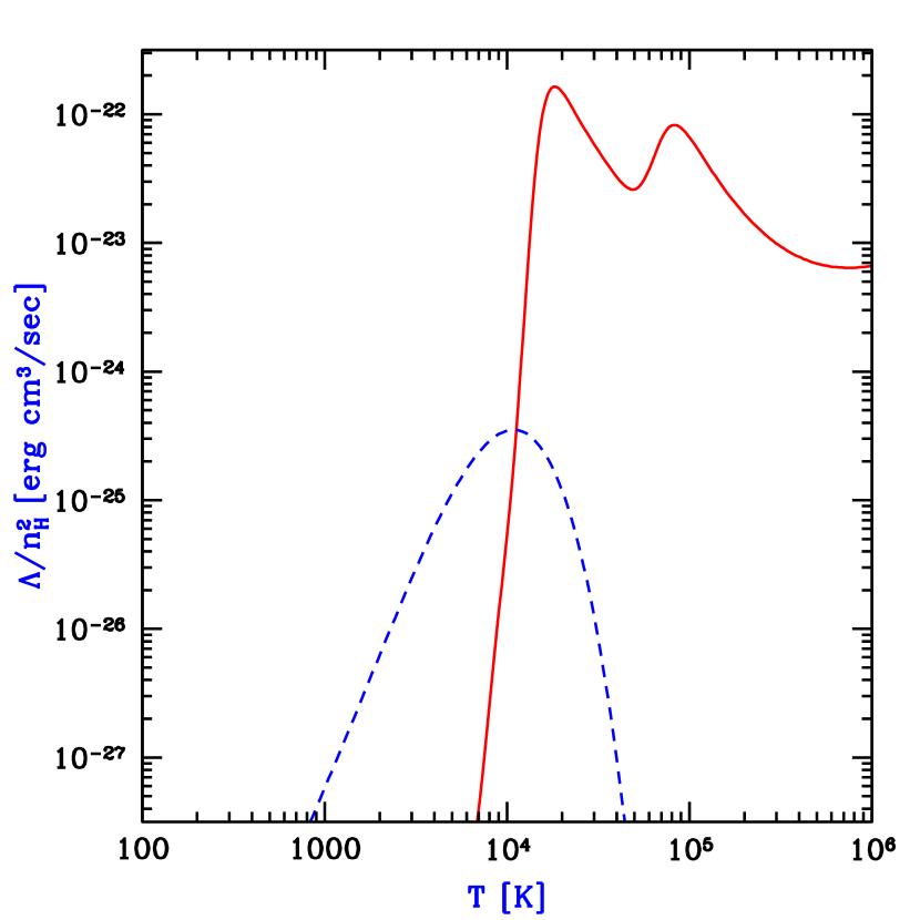
Figure 12: Cooling rates as a function of temperature for a primordial gas composed of atomic hydrogen and helium, as well as molecular hydrogen, in the absence of any external radiation. We assume a hydrogen number density $n_{H}=0.045\ {\rm cm}^{-3}$, corresponding to the mean density of virialized halos at $z=10$. The plotted quantity $\Lambda/n_{H}^{2}$ is roughly independent of density (unless $n_{H}\gg 10\ {\rm cm}^{-3}$), where $\Lambda$ is the volume cooling rate (in erg/sec/cm³). The solid line shows the cooling curve for an atomic gas, with the characteristic peaks due to collisional excitation of H 1 and He 2. The dashed line (calculated using the code of Abel available at http://logy.harvard.edu/tabel/PGas/cool.html) shows the additional contribution of molecular cooling, assuming a molecular abundance equal to $0.1\%$ of $n_{H}$.

Table 1: Reaction Rates for Hydrogen Species

		Rate Coefficient
	Reaction	(cm3s-1)	Reference
(1)	H + $e^{-}$ $\rightarrow$ H+ + $2e^{-}$	$5.85\times 10^{-11}T^{1/2}\mbox{exp}(-157,809.1/T)(1+T^{1/2}_{5})^{-1}$	1
(2)	H+ + $e^{-}$ $\rightarrow$ H + $h\nu$	$8.40\times 10^{-11}T^{-1/2}T_{3}^{-0.2}(1+T^{0.7}_{6})^{-1}$	1
(3)	H + $e^{-}$ $\rightarrow$ H- + $h\nu$	See expression in reference	2
(4)	H + H- $\rightarrow$ H2 + $e^{-}$	$1.30\times 10^{-9}$	1
(5)	H- + H+ $\rightarrow$ 2H	$7.00\times 10^{-7}T^{-1/2}$	1
(6)	H2 + $e^{-}$ $\rightarrow$ H + H-	$2.70\times 10^{-8}T^{-3/2}\mbox{exp}(-43,000/T)$	1
(7)	H2 + H $\rightarrow$ 3H	See expression in reference	1
(8)	H2 + H+ $\rightarrow$ H${}^{+}_{2}$ + H	$2.40\times 10^{-9}\mbox{exp}(-21,200/T)$	1
(9)	H2 + $e^{-}$ $\rightarrow$ 2H + $e^{-}$	$4.38\times 10^{-10}\mbox{exp}(-102,000/T)T^{0.35}$	1
(10)	H- + $e^{-}$ $\rightarrow$ H + $2e^{-}$	$4.00\times 10^{-12}T\,\mbox{exp}(-8750/T)$	1
(11)	H- + H $\rightarrow$ 2H + $e^{-}$	$5.30\times 10^{-20}T\,\mbox{exp}(-8750/T)$	1
(12)	H- + H+ $\rightarrow$ H${}^{+}_{2}$ + $e^{-}$	See expression in reference	1

References. — (1) Haiman, Thoul, & Loeb 1996; (2) Abel, et al. 1997.

Table 2: Reaction Rates for Deuterium Species

		Rate Coefficient
	Reaction	(cm3s-1)	Reference
(1)	D+ + $e^{-}$ $\rightarrow$ D + $h\nu$	$8.40\times 10^{-11}T^{-1/2}T_{3}^{-0.2}(1+T^{0.7}_{6})^{-1}$	1
(2)	D + H+ $\rightarrow$ D+ + H	$3.70\times 10^{-10}T^{0.28}\mbox{exp}(-43/T)$	3
(3)	D+ + H $\rightarrow$ D + H+	$3.70\times 10^{-10}T^{0.28}$	3
(4)	D+ + H2 $\rightarrow$ H+ + HD	$2.10\times 10^{-9}$	3
(5)	HD + H+ $\rightarrow$ H2 + D+	$1.00\times 10^{-9}\mbox{exp}(-464/T)$	3

References. — (1) Haiman, Thoul, & Loeb 1996; (3) Galli & Palla 1998.

Table 3: Radiative Cooling Processes in the Primordial Gas

		Cooling rate
	Cooling due to	(erg s-1 cm-3)	Reference
(1)	Molecular hydrogen	See expression in reference	1
(2)	Deuterium hydride (HD)	See expression in reference	2
(3)	Atomic H & He	See expression in reference	3
(4)	Compton scattering	$5.6\times 10^{-36}(1+z)^{4}n_{e}(T-T_{\rm CMB})$	4

Note. — $T$ is the gas temperature in K, $T_{3}=T/10^{3}~{}{\rm K}$, $T_{5}=T/10^{5}~{}{\rm K}$, $T_{6}=T/10^{6}~{}{\rm K}$, $n_{e}$ is the density of free electrons, $z$ is the redshift, and $T_{\rm CMB}=2.73\,(1+z)$ K is the temperature of the CMB.

References. — (1) Galli & Palla 1998; (2) Flower, Le Bourlot, Pineau des Forêts, & Roueff 2000; (3) Cen 1992; Verner & Ferland 1996; Ferland et al. 1992; Voronov 1997 (4) Ikeuchi & Ostriker 1986.

4 Fragmentation of the First Gaseous Objects

4.1 Star Formation

4.1.1 Fragmentation into Stars

As mentioned in the preface, the fragmentation of the first gaseous objects is a well-posed physics problem with well specified initial conditions, for a given power-spectrum of primordial density fluctuations. This problem is ideally suited for three-dimensional computer simulations, since it cannot be reliably addressed in idealized 1D or 2D geometries.

Recently, two groups have attempted detailed 3D simulations of the formation process of the first stars in a halo of $\sim 10^{6}M_{\odot}$ by following the dynamics of both the dark matter and the gas components, including H₂ chemistry and cooling (Deuterium is not expected to play a significant role; Bromm 2000). Bromm et al. (1999) have used a Smooth Particle Hydrodynamics (SPH) code to simulate the collapse of a top-hat overdensity with a prescribed solid-body rotation (corresponding to a spin parameter $\lambda=5\%$) and additional small perturbations with $P(k)\propto k^{-3}$ added to the top-hat profile. Abel et al. (2000) isolated a high-density filament out of a larger simulated cosmological volume and followed the evolution of its density maximum with exceedingly high resolution using an Adaptive Mesh Refinement (AMR) algorithm.

The generic results of Bromm et al. (1999; see also Bromm 2000) are illustrated in Figure 13. The collapsing region forms a disk which fragments into many clumps. The clumps have a typical mass $\sim 10^{2}$–$10^{3}M_{\odot}$. This mass scale corresponds to the Jeans mass for a temperature of $\sim 500$K and the density $\sim 10^{4}~{}{\rm cm^{-3}}$ where the gas lingers because its cooling time is longer than its collapse time at that point (see Figure 14). This characteristic density is determined by the fact that hydrogen molecules reach local thermodynamic equilibrium at this density. At lower densities, each collision leads to an excited state and to radiative cooling, so the overall cooling rate is proportional to the collision rate, and the cooling time is inversely proportional to the gas density. Above the density of $\sim 10^{4}~{}{\rm cm^{-3}}$, however, the relative occupancy of each excited state is fixed at the thermal equilibrium value (for a given temperature), and the cooling time is nearly independent of density (e.g., Lepp & Shull 1983). Each clump accretes mass slowly until it exceeds the Jeans mass and collapses at a roughly constant temperature (i.e., isothermally) due to H₂ cooling. The clump formation efficiency is high in this simulation due to the synchronized collapse of the overall top-hat perturbation.

Figure 13: Numerical results from Bromm et al. (1999), showing gas properties at $z=31.2$ for a collapsing slightly inhomogeneous top-hat region with a prescribed solid-body rotation. Each point in the figure is a gas particle in the simulation. (a) Free electron fraction (by number) vs. hydrogen number density (in cm^-3). At densities exceeding $n\sim 10^{3}$ cm^-3, recombination is very efficient, and the gas becomes almost completely neutral. (b) Molecular hydrogen fraction vs. number density. After a quick initial rise, the H₂ fraction approaches the asymptotic value of $f\sim 10^{-3}$, due to the H^- channel. (c) Gas temperature vs. number density. At densities below $\sim 1$ cm^-3, the gas temperature rises because of adiabatic compression until it reaches the virial value of $T_{vir}\simeq 5000$ K. At higher densities, cooling due to H₂ drives the temperature down again, until the gas settles into a quasi-hydrostatic state at $T\sim 500$ K and $n\sim 10^{4}$ cm^-3. Upon further compression due to accretion and the onset of gravitational collapse, the gas shows a further modest rise in temperature. (d) Jeans mass (in $M_{\odot}$) vs. number density. The Jeans mass reaches a value of $M_{J}\sim 10^{3}M_{\odot}$ for the quasi-hydrostatic gas in the center of the potential well, and reaches the resolution limit of the simulation, $M_{\rm res}\simeq 200M_{\odot}$, for densities close to $n=10^{8}$ cm^-3.

Figure 14: Gas and clump morphology at $z=28.9$ in the simulation of Bromm et al. (1999). Top row: The remaining gas in the diffuse phase. Bottom row: Distribution of clumps. The numbers next to the dots denote clump mass in units of $M_{\odot}$. Left panels: Face-on view. Right panels: Edge-on view. The length of the box is 30 pc. The gas has settled into a flattened configuration with two dominant clumps of mass close to $20,000M_{\odot}$. During the subsequent evolution, the clumps survive without merging, and grow in mass only slightly by accretion of surrounding gas.

Bromm (2000, Chapter 7) has simulated the collapse of one of the above-mentioned clumps with $\sim 1000M_{\odot}$ and demonstrated that it does not tend to fragment into sub-components. Rather, the clump core of $\sim 100M_{\odot}$ free-falls towards the center leaving an extended envelope behind with a roughly isothermal density profile. At very high gas densities, three-body reactions become important in the chemistry of H₂. Omukai & Nishi (1998) have included these reactions as well as radiative transfer and followed the collapse in spherical symmetry up to stellar densities. Radiation pressure from nuclear burning at the center is unlikely to reverse the infall as the stellar mass builds up. These calculations indicate that each clump may end up as a single massive star; however, it is possible that angular momentum or nuclear burning may eventually halt the monolithic collapse and lead to further fragmentation.

The Jeans mass (§3.1), which is defined based on small fluctuations in a background of uniform density, does not strictly apply in the context of collapsing gas cores. We can instead use a slightly modified critical mass known as the Bonnor-Ebert mass (Bonnor 1956; Ebert 1955). For baryons in a background of uniform density $\rho_{b}$, perturbations are unstable to gravitational collapse in a region more massive than the Jeans mass

$$M_{J}=2.9\,\frac{1}{\sqrt{\rho_{b}}}\,\left(\frac{kT}{G\mu m_{p}}\right)^{3/2}\ .$$ (52)

Instead of a uniform background, we consider a spherical, non-singular, isothermal, self-gravitating gas in hydrostatic equilibrium, i.e., a centrally-concentrated object which more closely resembles the gas cores found in the above-mentioned simulations. We consider a finite sphere in equilibrium with an external pressure. In this case, small fluctuations are unstable and lead to collapse if the sphere is more massive than the Bonnor-Ebert mass $M_{\rm BE}$, given by the same expression as equation (52) but with a different coefficient (1.2 instead of 2.9) and with $\rho_{b}$ denoting in this case the gas (volume) density at the surface of the sphere.

In their simulation, Abel et al. (2000) adopted the actual cosmological density perturbations as initial conditions. The simulation focused on the density peak of a filament within the IGM, and evolved it to very high densities (Figure 15). Following the initial collapse of the filament, a clump core formed with $\sim 200M_{\odot}$, amounting to only $\sim 1\%$ of the virialized gas mass. Subsequently due to slow cooling, the clump collapsed subsonically in a state close to hydrostatic equilibrium (see Figure 16). Unlike the idealized top-hat simulation of Bromm et al. (2000), the collapse of the different clumps within the filament is not synchronized. Once the first star forms at the center of the first collapsing clump, it is likely to affect the formation of other stars in its vicinity.

Figure 15: Zooming in on the core of a star forming region with the Adaptive Mesh Refinement simulation of Abel et al. (2000). The panels show different length scales, decreasing clockwise by an order of magnitude between adjacent panels. Note the large dynamic range of scales which are being resolved, from 6 kpc (top left panel) down to 10,000 AU (bottom left panel).

Figure 16: Gas profiles from the simulation of Abel et al. (2000). The cell size on the finest grid corresponds to $0.024$ pc, while the simulation box size corresponds to 6.4 kpc. Shown are spherically-averaged mass-weighted profiles around the baryon density peak shortly before a well defined fragment forms ($z=19.1$). Panel (a) shows the baryonic number density (solid line), enclosed gas mass in solar mass (thin solid line with circles), and the local Bonnor-Ebert mass $M_{\rm BE}$ (dashed line; see text). Panel (b) plots the molecular hydrogen fraction (by number) $f_{\rm H_{2}}$ (solid line) and the free electron fraction $x$ (dashed line). The H₂ cooling time, $t_{\rm H_{2}}$, the time it takes a sound wave to travel to the center, $t_{\rm cross}$, and the free-fall time $t_{\rm ff}=[3\pi/(32G\rho)]^{1/2}$ are given in panel (c). Panel (d) gives the temperature in K as a function of radius. The bottom panel gives the local sound speed, $c_{s}$ (solid line with circles), the root-mean-square radial velocities of the dark matter (dashed line) and the gas (dashed line with asterisks) as well as the root-mean-square gas velocity (solid line with square symbols). The vertical dotted line indicates the radius ($\sim 5$ pc) at which the gas has reached its minimum temperature allowed by H₂ cooling. The virial radius of the $5.6\times 10^{6}M_{\odot}$ halo is 106 pc.

If the clumps in the above simulations end up forming individual very massive stars, then these stars will likely radiate copious amounts of ionizing radiation (Carr, Bond, & Arnett 1984; Tumlinson & Shull 2000; Bromm et al. 2000) and expel strong winds. Hence, the stars will have a large effect on their interstellar environment, and feedback is likely to control the overall star formation efficiency. This efficiency is likely to be small in galactic potential wells which have a virial temperature lower than the temperature of photoionized gas, $\sim 10^{4}$K. In such potential wells, the gas may go through only a single generation of star formation, leading to a “suicidal” population of massive stars.

The final state in the evolution of these stars is uncertain; but if their mass loss is not too extensive, then they are likely to end up as black holes (Bond, Carr, & Arnett 1984; Fryer, Woosley, & Heger 2001). The remnants may provide the seeds of quasar black holes (Larson 1999). Some of the massive stars may end their lives by producing $\gamma$-ray bursts. If so then the broad-band afterglows of these bursts could provide a powerful tool for probing the epoch of reionization (Lamb & Reichart 2000; Ciardi & Loeb 2000). There is no better way to end the dark ages than with $\gamma$-ray burst fireworks.

Where are the first stars or their remnants located today? The very first stars formed in rare high-$\sigma$ peaks and hence are likely to populate the cores of present-day galaxies (White & Springel 1999). However, the star clusters which formed in low-$\sigma$ peaks at later times are expected to behave similarly to the collisionless dark matter particles and populate galaxy halos (Loeb 1998).

4.1.2 Emission Spectrum of Metal-Free Stars

The evolution of metal-free (Population III) stars is qualitatively different from that of enriched (Population I and II) stars. In the absence of the catalysts necessary for the operation of the CNO cycle, nuclear burning does not proceed in the standard way. At first, hydrogen burning can only occur via the inefficient PP chain. To provide the necessary luminosity, the star has to reach very high central temperatures ($T_{c}\simeq 10^{8.1}$ K). These temperatures are high enough for the spontaneous turn-on of helium burning via the triple-$\alpha$ process. After a brief initial period of triple-$\alpha$ burning, a trace amount of heavy elements forms. Subsequently, the star follows the CNO cycle. In constructing main-sequence models, it is customary to assume that a trace mass fraction of metals ($Z\sim 10^{-9}$) is already present in the star (El Eid et al. 1983; Castellani et al. 1983).

Figures 17 and 18 show the luminosity $L$ vs. effective temperature $T$ for zero-age main sequence stars in the mass ranges of $2$–$90M_{\odot}$ (Figure 17) and $100$–$1000M_{\odot}$ (Figure 18). Note that above $\sim 100M_{\odot}$ the effective temperature is roughly constant, $T_{\rm eff}\sim 10^{5}$K, implying that the spectrum is independent of the mass distribution of the stars in this regime (Bromm et al. 2000). As is evident from these Figures (see also Tumlinson & Shull 2000), both the effective temperature and the ionizing power of metal-free (Pop III) stars are substantially larger than those of metal-rich (Pop I) stars. Metal-free stars with masses $\gtrsim 20M_{\odot}$ emit between $10^{47}$ and $10^{48}$ H 1 and He 1 ionizing photons per second per solar mass of stars, where the lower value applies to stars of $\sim 20M_{\odot}$ and the upper value applies to stars of $\gtrsim 100M_{\odot}$ (see Tumlinson & Shull 2000 and Bromm et al. 2000 for more details). These massive stars produce $10^{4}$–$10^{5}$ ionizing photons per stellar baryon over a lifetime of $\sim 3\times 10^{6}$ years [which is much shorter than the age of the universe, equation (10) in §2.1]. However, this powerful UV emission is suppressed as soon as the interstellar medium out of which new stars form is enriched by trace amounts of metals. Even though the collapsed fraction of baryons is small at the epoch of reionization, it is likely that most of the stars responsible for the reionization of the universe formed out of enriched gas.

Figure 17: Luminosity vs. effective temperature for zero-age main sequences stars in the mass range of $2$–$90M_{\odot}$ (from Tumlinson & Shull 2000). The curves show Pop I ($Z_{\odot}$ = 0.02, on the right) and Pop III stars (on the left) in the mass range 2–90 $M_{\odot}$. The diamonds mark decades in metallicity in the approach to $Z=0$ from 10^-2 down to 10^-5 at 2 $M_{\odot}$, down to 10^-10 at 15 $M_{\odot}$, and down to 10^-13 at 90 $M_{\odot}$. The dashed line along the Pop III zero-age main sequence assumes pure H-He composition, while the solid line (on the left) marks the upper MS with $Z_{\rm C}=10^{-10}$ for the $M\geq 15$ $M_{\odot}$ models. Squares mark the points corresponding to pre-enriched evolutionary models from El Eid et al. (1983) at 80 $M_{\odot}$ and from Castellani et al. (1983) at 25 $M_{\odot}$.

Figure 18: Same as Figure 17 but for very massive stars above $100M_{\odot}$ (from Bromm et al. 2000). Left solid line: Pop III zero-age main sequence (ZAMS). Right solid line: Pop I ZAMS. In each case, stellar luminosity (in $L_{\odot}$) is plotted vs. effective temperature (in K). Diamond-shaped symbols: Stellar masses along the sequence, from $100M_{\odot}$ (bottom) to $1000M_{\odot}$ (top) in increments of $100M_{\odot}$. The Pop III ZAMS is systematically shifted to higher effective temperature, with a value of $\sim 10^{5}$ K which is approximately independent of mass. The luminosities, on the other hand, are almost identical in the two cases.

Will it be possible to infer the initial mass function (IMF) of the first stars from spectroscopic observations of the first galaxies? Figure 19 compares the observed spectrum from a Salpeter IMF ($dN_{\star}/dM\propto M^{-2.35}$) and a heavy IMF (with all stars more massive than $100M_{\odot}$) for a galaxy at $z_{s}=10$. The latter case follows from the assumption that each of the dense clumps in the simulations described in the previous section ends up as a single star with no significant fragmentation or mass loss. The difference between the plotted spectra cannot be confused with simple reddening due to normal dust. Another distinguishing feature of the IMF is the expected flux in the hydrogen and helium recombination lines, such as Ly$\alpha$ and He 2 1640 Å, from the interstellar medium surrounding these stars. We discuss this next.

Figure 19: Comparison of the predicted flux from a Pop III star cluster at $z_{s}=10$ for a Salpeter IMF (Tumlinson & Shull 2000) and a massive IMF (Bromm et al. 2000). Plotted is the observed flux (in nJy per $10^{6}M_{\odot}$ of stars) vs. observed wavelength (in $\mu$m) for a flat universe with $\Omega_{\Lambda}=0.7$ and $h=0.65$. Solid line: The case of a heavy IMF. Dotted line: The fiducial case of a standard Salpeter IMF. The cutoff below $\lambda_{obs}=1216\mbox{\,\AA\,}(1+z_{s})=1.34\mu$m is due to Gunn-Peterson absorption. (The cutoff has been slightly smoothed here by the damping wing of the Ly$\alpha$ line, with reionization assumed to occur at $z=7$; see §9.1.1 for details.) Clearly, for the same total stellar mass, the observable flux is larger by an order of magnitude for stars which are biased towards having masses $\gtrsim 100M_{\odot}\,$.

4.1.3 Emission of Recombination Lines from the First Galaxies

The hard UV emission from a star cluster or a quasar at high redshift is likely reprocessed by the surrounding interstellar medium, producing very strong recombination lines of hydrogen and helium (Oh 1999; Tumlinson & Shull 2000; see also Baltz, Gnedin & Silk 1998). We define $\dot{N}_{\rm ion}$ to be the production rate per unit stellar mass of ionizing photons by the source. The emitted luminosity $L_{\rm line}^{\rm em}$ per unit stellar mass in a particular recombination line is then estimated to be

$$L_{\rm line}^{\rm em}=p_{\rm line}^{\rm em}h\nu\dot{N}_{\rm ion}(1-p^{\rm esc}_{\rm cont})p^{\rm esc}_{\rm line}\mbox{\ \ \ ,}$$ (53)

where $p_{\rm line}^{\rm em}$ is the probability that a recombination leads to the emission of a photon in the corresponding line, $\nu$ is the frequency of the line and $p^{\rm esc}_{\rm cont}$ and $p^{\rm esc}_{\rm line}$ are the escape probabilities for the ionizing photons and the line photons, respectively. It is natural to assume that the stellar cluster is surrounded by a finite H 2 region, and hence that $p^{\rm esc}_{\rm cont}$ is close to zero (Wood & Loeb 2000; Ricotti & Shull 2000). In addition, $p^{\rm esc}_{\rm line}$ is likely close to unity in the H 2 region, due to the lack of dust in the ambient metal-free gas. Although the emitted line photons may be scattered by neutral gas, they diffuse out to the observer and in the end survive if the gas is dust free. Thus, for simplicity, we adopt a value of unity for $p^{\rm esc}_{\rm line}$ (two-photon decay is generally negligible as a way of losing line photons in these environments).

As a particular example we consider case B recombination which yields $p_{\rm line}^{\rm em}$ of about 0.65 and 0.47 for the Ly${\alpha}$ and He 2 1640 Å lines, respectively. These numbers correspond to an electron temperature of $\sim 3\times 10^{4}$K and an electron density of $\sim 10^{2}-10^{3}$ cm^-3 inside the H 2 region (Storey & Hummer 1995). For example, we consider the extreme and most favorable case of metal-free stars all of which are more massive than $\sim 100M_{\odot}$. In this case $L_{\rm line}^{\rm em}=1.7\times 10^{37}$ and $2.2\times 10^{36}$ erg s${}^{-1}M_{\odot}^{-1}$ for the recombination luminosities of Ly$\alpha$ and He 2 1640 Å per stellar mass (Bromm et al. 2000). A cluster of $10^{6}M_{\odot}$ in such stars would then produce 4.4 and 0.6 $\times 10^{9}L_{\odot}$ in the Ly$\alpha$ and He 2 1640 Å lines. Comparably-high luminosities would be produced in other recombination lines at longer wavelengths, such as He 2 4686 Å and H$\alpha$ (Oh 2000; Oh, Haiman, & Rees 2000).

The rest-frame equivalent width of the above emission lines measured against the stellar continuum of the embedded star cluster at the line wavelengths is given by

$$W_{\lambda}=\left(\frac{L_{\rm line}^{\rm em}}{L_{\lambda}}\right)\mbox{\ \ \ ,}$$ (54)

where $L_{\lambda}$ is the spectral luminosity per unit wavelength of the stars at the line resonance. The extreme case of metal-free stars which are more massive than $100M_{\odot}$ yields a spectral luminosity per unit frequency $L_{\nu}=2.7\times 10^{21}$ and $1.8\times 10^{21}$ erg s^-1 Hz${}^{-1}M_{\odot}^{-1}$ at the corresponding wavelengths (Bromm et al. 2000). Converting to $L_{\lambda}$, this yields rest-frame equivalent widths of $W_{\lambda}$ = 3100 Å and 1100 Å for Ly$\alpha$ and He 2 1640 Å, respectively. These extreme emission equivalent widths are more than an order of magnitude larger than the expectation for a normal cluster of hot metal-free stars with the same total mass and a Salpeter IMF under the same assumptions concerning the escape probabilities and recombination (Kudritzki et al. 2000). The equivalent widths are, of course, larger by a factor of $(1+z_{s})$ in the observer frame. Extremely strong recombination lines, such as Ly$\alpha$ and He 2 1640 Å, are therefore expected to be an additional spectral signature that is unique to very massive stars in the early universe. The strong recombination lines from the first luminous objects are potentially detectable with NGST  (Oh, Haiman, & Rees 2000).

High-redshift objects could also, in principle, be detected through their cooling radiation. However, a simple estimate of the radiated energy shows that it is very difficult to detect the corresponding signal in practice. As it cools, the gas loses much of its gravitational binding energy, which is of order $k_{B}T_{\rm vir}$ per baryon, with the virial temperature given by equation (26) in §2.3. Some fraction of this energy is then radiated as Ly$\alpha$ photons. The typical galaxy halos around the reionization redshift have $T_{\rm vir}\sim 1$ eV, and this must be compared to the nuclear energy output of 7 MeV per baryon in stellar interiors. Clearly, for a star formation efficiency of $\gtrsim 1\%$, the stellar radiation is expected to be far more energetic than the cooling radiation. Both forms of energy should come out on a time-scale of order the dynamical time. Thus, even if the cooling radiation is concentrated in the Ly$\alpha$ line, its detection is more promising for low redshift objects, while NGST  will only be able to detect this radiation from the rare 4-$\sigma$ halos (with masses $\gtrsim 10^{1}1M_{\sun}$) at $z\sim 10$ (Haiman, Spaans, & Quataert 2000; Fardal et al. 2000).

4.2 Black Hole Formation

Quasars are more effective than stars in ionizing the intergalactic hydrogen because (i) their emission spectrum is harder, (ii) the radiative efficiency of accretion flows can be more than an order of magnitude higher than the radiative efficiency of a star, and (iii) quasars are brighter, and for a given density distribution in their host system, the escape fraction of their ionizing photons is higher than for stars.

Thus, the history of reionization may have been greatly altered by the existence of massive black holes in the low-mass galaxies that populate the universe at high redshifts. For this reason, it is important to understand the formation of massive black holes (i.e., black holes with a mass far greater than a stellar mass). The problem of black hole formation is not a priori more complicated than the problem of star formation. Surprisingly, however, the amount of theoretical work on star formation far exceeds that on massive black hole formation. One of the reasons is that stars form routinely in our interstellar neighborhood where much data can be gathered, while black holes formed mainly in the distant past at great distances from our telescopes. As more information is gathered on the high-redshift universe, this state of affairs may begin to change.

Here we adopt the view that massive black holes form out of gas and not through the dynamical evolution of dense stellar systems (see Rees 1984 for a review of the alternatives). To form a black hole inside a given dark matter halo, the baryons must cool. For most objects, this is only possible with atomic line cooling at virial temperatures $T_{\rm vir}\gtrsim 10^{4}$K and thus baryonic masses $\gtrsim 10^{7}M_{\odot}[(1+z)/10]^{3/2}$. After losing their thermal pressure, the cold baryons collapse and form a thin disk on a dynamical time (Loeb & Rasio 1994). The basic question is then the following: what fraction of the cold baryons is able to sink to the very center of the potential well and form a massive black hole? Just as for star formation, the main barrier in this process is angular momentum. The centrifugal force opposes radial infall and keeps the gas in disks at a typical distance which is 6–8 orders of magnitude larger than the Schwarzschild radius corresponding to the total gas mass. Eisenstein & Loeb (1995b) demonstrated that a small fraction of all objects have a sufficiently low angular momentum that the gas in them inevitably forms a compact semi-relativistic disk that evolves to a black hole on a short viscous time-scale. These low-spin systems are born in special cosmological environments that exert unusually small tidal torques on them during their cosmological collapse. As long as the initial cooling time of the gas is short and its star formation efficiency is low, the gas forms the compact disk on a free-fall time. In most systems the baryons dominate gravity inside the scale length of the disk. Therefore, if the baryons in a low-spin system acquire a spin parameter which is only one sixth of the typical value, i.e., an initial rotation speed $\sim(16\%\times 0.05)\times V_{c}$, then with angular momentum conservation they would reach rotational support at a radius $r_{\rm disk}$ and circular velocity $V_{\rm disk}$ such that $V_{\rm disk}\,r_{\rm disk}\sim(16\%\times 0.05)\,V_{c}\,r_{\rm vir}$, where $r_{\rm vir}$ is the virial radius and $V_{c}$ the circular velocity of the halo. Using the relations: $(GM_{\rm halo}/r_{\rm vir})\sim V_{c}^{2}$, and $[G(\Omega_{b}/\Omega_{m})M_{\rm halo}/r_{\rm disk}]\sim V_{\rm disk}^{2}$, we get $V_{\rm disk}\sim 18V_{c}$. For $T_{\rm vir}\sim 10^{4}$K, the dark matter halo has a potential depth corresponding to a circular velocity of $V_{c}\sim 17~{}{\rm km~{}s^{-1}}$, and the low-spin disk attains a characteristic rotation velocity of $V_{\rm disk}\sim 300~{}{\rm km~{}s^{-1}}$ (sufficient to retain the gas against supernova-driven winds), a size $\lesssim\,1$ pc, and a viscous evolution time which is extremely short compared to the Hubble time.

Low-spin dwarf galaxies populate the universe with a significant volume density at high redshift; these systems are eventually incorporated into higher mass galaxies which form later. For example, a galactic bulge of $\sim 10^{10}M_{\odot}$ in baryons forms out of $\sim 10^{3}$ building blocks of $\sim 10^{7}M_{\odot}$ each. In order to seed the growth of a quasar, it is sufficient that only one of these systems had formed a low-spin disk that produced a black hole progenitor. Note that if a low-spin object is embedded in an overdense region that eventually becomes a galactic bulge, then the black hole progenitor will sink to the center of the bulge by dynamical friction in less than a Hubble time (for a sufficiently high mass $\gtrsim 10^{6}M_{\sun}\,$; p. 428 of Binney & Tremaine) and seed quasar activity. Based on the phase-space volume accessible to low-spin systems ($\propto j^{3}$), we expect a fraction $\sim 6^{-3}=5\times 10^{-3}$ of all the collapsed gas mass in the universe to be associated with low-spin disks (Eisenstein & Loeb 1995b). However, this is a conservative estimate. Additional angular momentum loss due to dynamical friction of gaseous clumps in dark matter halos (Navarro, Frenk, & White 1995) or bar instabilities in self-gravitating disks (Shlosman, Begelman, & Frank 1990) could only contribute to the black hole formation process. The popular paradigm that all galaxies harbor black holes at their center simply postulates that in all massive systems, a small fraction of the gas ends up as a black hole, but does not explain quantitatively why this fraction obtains its particular small value. The above scenario offers a possible physical context for this result.

If the viscous evolution time is shorter than the cooling time and if the gas entropy is raised by viscous dissipation or shocks to a sufficiently high value, then the black hole formation process will go through the phase of a supermassive star (Shapiro & Teukolsky 1983, §17; see also Zel’dovich & Novikov 1971). The existence of angular momentum (Wagoner 1969) tends to stabilize the collapse against the instability which itself is due to general-relativistic corrections to the Newtonian potential (Shapiro & Teukolsky 1983, §17.4). However, shedding of mass and angular momentum along the equatorial plane eventually leads to collapse (Bisnovati-Kogan, Zel’dovich & Novikov 1967; Loeb & Rasio 1994; Baumgarte & Shapiro 1999a). Since it is convectively unstable (Loeb & Rasio 1994) and supported by radiation pressure, a supermassive star should radiate close to the Eddington limit (with modifications due to rotation; see Baumgarte & Shapiro 1999b) and generate a strong wind, especially if the gas is enriched with metals. The thermal$+$wind emission associated with the collapse of a supermassive star should be short-lived and could account for only a minority of all observed quasars.

After the seed black hole forms, it is continually fed with gas during mergers. Mihos & Hernquist (1996) have demonstrated that mergers tend to deposit large quantities of gas at the centers of the merging galaxies, a process which could fuel a starburst or a quasar. If both of the merging galaxies contain black holes at their centers, dynamical friction will bring the black holes together. The final spiral-in of the black hole binary depends on the injection of new stars into orbits which allow them to extract angular momentum from the binary (Begelman, Blandford, & Rees 1980). If the orbital radius of the binary shrinks to a sufficiently small value, gravitational radiation takes over and leads to coalescence of the two black holes. This will provide powerful sources for future gravitational wave detectors (such as the LISA project; see http://lisa.jpl.nasa.gov).

The fact that black holes are found in low-mass galaxies in the local universe implies that they are likely to exist also at high redshift. Local examples include the compact ellipticals M32 and NGC 4486B. In particular, van der Marel et al. (1997) infer a black hole mass of $\sim 3.4\times 10^{6}M_{\odot}$ in M32, which is a fraction $\sim 8\times 10^{-3}$ of the stellar mass of the galaxy, $\sim 4\times 10^{8}M_{\odot}$, for a central mass-to-light ratio of $\gamma_{V}=2$. In NGC 4486B, Kormendy et al. (1997) infer a black hole mass of $6\times 10^{8}M_{\odot}$, which is a fraction $\sim 9\%$ of the stellar mass.

Despite the poor current understanding of the black hole formation process, it is possible to formulate reasonable phenomenological prescriptions that fit the quasar luminosity function within the context of popular galaxy formation models. These prescription are described in §8.2.2.

5 Galaxy Properties

5.1 Formation and Properties of Galactic Disks

The formation of disk galaxies within hierarchical models of structure formation was first explored by Fall & Efstathiou (1980). More recently, the distribution of disk sizes was derived and compared to observations by Dalcanton, Spergel, & Summers (1997) and Mo, Mao, & White (1998). Although these authors considered a number of detailed models, we adopt here the simple model of an exponential disk in a singular isothermal sphere halo. We consider a halo of mass $M$, virial radius $r_{\rm vir}$, total energy $E$, and angular momentum $J$, for which the spin parameter is defined as

$$\lambda\equiv J|E|^{1/2}G^{-1}M^{-5/2}\ .$$ (55)

The spin parameter simply expresses the halo angular momentum in a dimensionless form. The gas disk is assumed to collapse to a state of rotational support in the dark matter halo. If the disk mass is a fraction $m_{d}$ of the halo mass and its angular momentum is a fraction $j_{d}$ of that of the halo, then the exponential scale radius of the disk is given by (Mo et al. 1998)

$$R_{d}=\frac{1}{\sqrt{2}}\left(\frac{j_{d}}{m_{d}}\right)\lambda\,r_{\rm vir}\ .$$ (56)

The observed distribution of disk sizes suggests that the specific angular momentum of the disk is similar to that of the halo (e.g., Dalcanton et al. 1997; Mo et al. 1998), and so we assume that $j_{d}/m_{d}=1$. Although this result is implied by observed galactic disks, its origin in the disk formation process is still unclear. The formation of galactic disks has been investigated in a large number of numerical simulations (Navarro & Benz 1991; Evrard, Summers, & Davis 1994; Navarro, Frenk, & White 1995; Tissera, Lambas, & Abadi 1997; Navarro & Steinmetz 1997; Elizondo, et al. 1999). The overall conclusion is that the collapsing gas loses angular momentum to the dark matter halo during mergers, and the disks which form are much smaller than observed galactic disks. The most widely discussed solution for this problem is to prevent the gas from collapsing into a disk by injecting energy through supernova feedback (e.g. Eke, Efstathiou, & Wright 1999; Binney, Gerhard, & Silk 2001; Efstathiou 2000). However, some numerical simulations suggest that feedback may not adequately suppress the angular momentum losses (Navarro & Steinmetz 2000).

With the assumption that $j_{d}/m_{d}=1$, the distribution of disk sizes is then determined by the Press-Schechter halo abundance and by the distribution of spin parameters [along with equation (24) for $r_{\rm vir}$]. The spin parameter distribution is approximately independent of mass, environment, and cosmological parameters, apparently a consequence of the scale-free properties of the early tidal torques between neighboring systems responsible for the spin of individual halos (Peebles 1969; White 1984; Barnes & Efstathiou 1987; Heavens & Peacock 1988; Steinmetz & Bartelmann 1995; Eisenstein & Loeb 1995a; Cole & Lacey 1996; Catelan & Theuns 1996). This distribution approximately follows a lognormal distribution in the vicinity of the peak,

$$p(\lambda)d\lambda=\frac{1}{\sigma_{\lambda}\sqrt{2\pi}}\exp\left[-\frac{\ln^{2}(\lambda/\bar{\lambda})}{2\sigma_{\lambda}^{2}}\right]\frac{d\lambda}{\lambda}\ ,$$ (57)

with $\bar{\lambda}=0.05$ and $\sigma_{\lambda}=0.5$ following Mo et al. (1998), who determined these values based on the N-body simulations of Warren et al. (1992). Although Mo et al. (1998) suggest a lower cutoff on $\lambda$ due to disk instability, it is unclear if halos with low $\lambda$ indeed cannot contain disks. If a dense bulge exists, it can prevent bar instabilities, or if a bar forms it may be weakened or destroyed when a bulge subsequently forms (Sellwood & Moore 1999).

5.2 Phenomenological Prescription for Star Formation

Schmidt (1959) put forth the hypothesis that the rate of star formation in a given region varies as a power of the gas density within that region. Thus, the star formation rate can be parameterized as

$$\frac{d\rho_{*}}{dt}\propto\rho_{g}^{N}\ ,$$ (58)

where $\rho_{*}$ is the mass density of stars, and $\rho_{g}$ is the mass density of gas. Although Schmidt originally focused on different regions within our own Galaxy, this relation has since been used to interpret observations of the global star formation rates in different galaxies.

One particular value of $N$ is theoretically favored for self-gravitating disks (e.g., Larson 1992; Elmegreen 1994). The star formation rate can be written in the form

$$\frac{d\rho_{*}}{dt}=\epsilon\frac{\rho_{g}}{t_{c}}\ ,$$ (59)

where $\epsilon$ is an efficiency coefficient, and $t_{c}$ is a characteristic time for star formation. If $t_{c}$ is proportional to the dynamical free-fall time, i.e., $t_{c}\propto\rho_{g}^{-1/2}$, then $N=1.5$. However, observations yield estimates of surface densities $\Sigma$, not volume densities $\rho$. If the average gas scale height is roughly constant in different environments, then the same relation as equation (58) should hold between the surface densities of stars and gas, with $N=1.5$.

Such a relation has, indeed, been observed to hold over a large range of physical conditions in galaxies. Synthetic models which include stellar evolution tracks and stellar atmosphere models are used to infer star formation rates using spectral observations of stellar populations. Star formation rates have been inferred in this way in the disks of normal spiral and irregular galaxies, most often using H_α luminosities. Star formation also occurs in much denser environments in the nuclear regions of galaxies, where far-infrared luminosities are most useful for determining star formation rates. Thus, the relation between star formation and gas density has been measured over conditions ranging from the outskirts of normal disks to the central engines of infrared-luminous starburst galaxies. The result is a tight correlation in accordance with the Schmidt law, empirically given by (Kennicutt 1998)

$$\Sigma_{SFR}=(2.5\pm 0.7)\times 10^{-4}\left[\frac{\Sigma_{gas}}{1M_{\sun}{\rm pc}^{-2}}\right]^{1.4\pm 0.15}M_{\sun}\,{\rm yr}^{-1}\,{\rm kpc}^{-2}\ ,$$ (60)

where $\Sigma_{SFR}$ and $\Sigma_{gas}$ are the disk-averaged star formation rate and gas surface densities, respectively. This relation is observed to hold over almost five orders of magnitude in gas surface density.

6 Radiative Feedback from the First Sources of Light

6.1 Escape of Ionizing Radiation from Galaxies

The intergalactic ionizing radiation field, a key ingredient in the development of reionization, is determined by the amount of ionizing radiation escaping from the host galaxies of stars and quasars. The value of the escape fraction as a function of redshift and galaxy mass remains a major uncertainty in all current studies, and could affect the cumulative radiation intensity by orders of magnitude at any given redshift. Gas within halos is far denser than the typical density of the IGM, and in general each halo is itself embedded within an overdense region, so the transfer of the ionizing radiation must be followed in the densest regions in the universe. Numerical simulations of reionization are limited in their resolution of the densest regions and in the accuracy of their treatment of radiative transfer.

The escape of ionizing radiation ($h\nu>13.6$eV, $\lambda<912$ Å) from the disks of present-day galaxies has been studied in recent years in the context of explaining the extensive diffuse ionized gas layers observed above the disk in the Milky Way (Reynolds et al. 1995) and other galaxies (e.g., Rand 1996; Hoopes, Walterbos, & Rand 1999). Theoretical models predict that of order 3–14% of the ionizing luminosity from O and B stars escapes the Milky Way disk (Dove & Shull 1994; Dove, Shull, & Ferrara 2000). A similar escape fraction of $f_{\rm esc}=6$% was determined by Bland-Hawthorn & Maloney (1999) based on H$\alpha$ measurements of the Magellanic Stream. From Hopkins Ultraviolet Telescope observations of four nearby starburst galaxies (Leitherer et al. 1995; Hurwitz, Jelinsky, & Dixon 1997), the escape fraction was estimated to be in the range 3%$<f_{\rm esc}<57$%. If similar escape fractions characterize high-redshift galaxies, then stars could have provided a major fraction of the background radiation that reionized the IGM (e.g., Madau & Shull 1996; Madau 1999). However, the escape fraction from high-redshift galaxies, which formed when the universe was much denser ($\rho\propto(1+z)^{3}$), may be significantly lower than that predicted by models meant to describe present-day galaxies. Current reionization calculations assume that galaxies are isotropic point sources of ionizing radiation and adopt escape fractions in the range $5\%<f_{\rm esc}<60\%$ (see, e.g., Gnedin 2000a, Miralda-Escudé et al. 2000).

Clumping is known to have a significant effect on the penetration and escape of radiation from an inhomogeneous medium (e.g., Boissé 1990; Witt & Gordon 1996, 2000; Neufeld 1991; Haiman & Spaans 1999; Bianchi et al. 2000). The inclusion of clumpiness introduces several unknown parameters into the calculation, such as the number and overdensity of the clumps, and the spatial correlation between the clumps and the ionizing sources. An additional complication may arise from hydrodynamic feedback, whereby part of the gas mass is expelled from the disk by stellar winds and supernovae (§7).

Wood & Loeb (2000) used a three-dimensional radiation transfer code to calculate the steady-state escape fraction of ionizing photons from disk galaxies as a function of redshift and galaxy mass. The gaseous disks were assumed to be isothermal, with a sound speed $c_{s}\sim 10~{}{\rm km~{}s^{-1}}$, and radially exponential, with a scale-length based on the characteristic spin parameter and virial radius of their host halos. The corresponding temperature of $\sim 10^{4}$ K is typical for a gas which is continuously heated by photo-ionization from stars. The sources of radiation were taken to be either stars embedded in the disk, or a central quasar. For stellar sources, the predicted increase in the disk density with redshift resulted in a strong decline of the escape fraction with increasing redshift. The situation is different for a central quasar. Due to its higher luminosity and central location, the quasar tends to produce an ionization channel in the surrounding disk through which much of its ionizing radiation escapes from the host. In a steady state, only recombinations in this ionization channel must be balanced by ionizations, while for stars there are many ionization channels produced by individual star-forming regions and the total recombination rate in these channels is very high. Escape fractions $\gtrsim 10\%$ were achieved for stars at $z\sim 10$ only if $\sim 90\%$ of the gas was expelled from the disks or if dense clumps removed the gas from the vast majority ($\gtrsim 80\%$) of the disk volume (see Figure 20). This analysis applies only to halos with virial temperatures $\gtrsim 10^{4}$ K. Ricotti & Shull (2000) reached similar conclusions but for a quasi-spherical configuration of stars and gas. They demonstrated that the escape fraction is substantially higher in low-mass halos with a virial temperature $\lesssim 10^{4}$ K. However, the formation of stars in such halos depends on their uncertain ability to cool via the efficient production of molecular hydrogen (see §3.3).

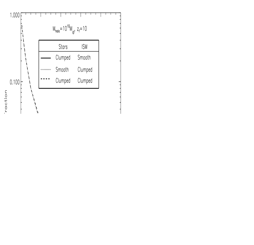
Figure 20: Escape fractions of stellar ionizing photons from a gaseous disk embedded within a $10^{10}M_{\odot}$ halo which formed at $z=10$ (from Wood & Loeb 2000). The curves show three different cases of clumpiness within the disk. The volume filling factor refers to either the ionizing emissivity, the gas clumps, or both, depending on the case. The escape fraction is substantial ($\gtrsim 1\%$) only if the gas distribution is highly clumped. (Note: ISM is interstellar medium)

The main uncertainty in the above predictions involves the distribution of the gas inside the host galaxy, as the gas is exposed to the radiation released by stars and the mechanical energy deposited by supernovae. Given the fundamental role played by the escape fraction, it is desirable to calibrate its value observationally. Recently, Steidel, Pettini, & Adelberger (2001) reported a preliminary detection of significant Lyman continuum flux in the composite spectrum of 29 Lyman break galaxies (LBG) with redshifts in the range $z=3.40\pm 0.09$. They co-added the spectra of these galaxies in order to be able to measure the low flux. Another difficulty in the measurement comes from the need to separate the Lyman-limit break caused by the interstellar medium from that already produced in the stellar atmospheres. After correcting for intergalactic absorption, Steidel et al. (2001) inferred a ratio between the emergent flux density at 1500Å  and 900Å  (rest frame) of $4.6\pm 1.0$. Taking into account the fact that the stellar spectrum should already have an intrinsic Lyman discontinuity of a factor of $\sim 3$–5, but that only $\sim 15$–$20\%$ of the 1500Å  photons escape from typical LBGs without being absorbed by dust (Pettini et al. 1998a; Adelberger & Steidel 2000), the inferred 900Å  escape fraction is $f_{\rm esc}\sim 10$–$20\%$. However, the observed blue spectrum suggests that these 29 particular LBGs may have a very low dust content, and the escape fraction in these galaxies may be $50\%$ or higher (Haehnelt et al. 2001). Thus, although the galaxies in this sample were drawn from the bluest quartile of the LBG spectral energy distributions, the measurement implies that this quartile may itself dominate the hydrogen-ionizing background relative to quasars at $z\sim 3$.

6.2 Propagation of Ionization Fronts in the IGM

The radiation output from the first stars ionizes hydrogen in a growing volume, eventually encompassing almost the entire IGM within a single H 2 bubble. In the early stages of this process, each galaxy produces a distinct H 2 region, and only when the overall H 2 filling factor becomes significant do neighboring bubbles begin to overlap in large numbers, ushering in the “overlap phase” of reionization. Thus, the first goal of a model of reionization is to describe the initial stage, when each source produces an isolated expanding H 2 region.

We assume a spherical ionized volume $V$, separated from the surrounding neutral gas by a sharp ionization front. In the case of a stellar ionizing spectrum, most ionizing photons are just above the hydrogen ionization threshold of 13.6 eV, where the absorption cross-section is high and a very thin layer of neutral hydrogen is sufficient to absorb all the ionizing photons. On the other hand, an ionizing source such as a quasar produces significant numbers of higher energy photons and results in a thicker transition region.

In the absence of recombinations, each hydrogen atom in the IGM would only have to be ionized once, and the ionized proper volume $V_{p}$ would simply be determined by

$$\bar{n}_{H}V_{p}=N_{\gamma}\ ,$$ (61)

where $\bar{n}_{H}$ is the mean number density of hydrogen and $N_{\gamma}$ is the total number of ionizing photons produced by the source. However, the increased density of the IGM at high redshift implies that recombinations cannot be neglected. Indeed, in the case of a steady ionizing source (and neglecting the cosmological expansion), a steady-state volume would be reached corresponding to the Strömgren sphere, with recombinations balancing ionizations:

$$\alpha_{B}\bar{n}_{H}^{2}V_{p}=\frac{d\,N_{\gamma}}{dt}\ ,$$ (62)

where the recombination rate depends on the square of the density and on the case B recombination coefficient $\alpha_{B}=2.6\times 10^{-13}$ cm³ s^-1 for hydrogen at $T=10^{4}$ K. The exact evolution for an expanding H 2 region, including a non-steady ionizing source, recombinations, and cosmological expansion, is given by (Shapiro & Giroux 1987)

$$\bar{n}_{H}\left(\frac{dV_{p}}{dt}-3HV_{p}\right)=\frac{d\,N_{\gamma}}{dt}-\alpha_{B}\left<n_{H}^{2}\right>V_{p}\ .$$ (63)

In this equation, the mean density $\bar{n}_{H}$ varies with time as $1/a^{3}(t)$. A critical feature of the physics of reionization is the dependence of recombination on the square of the density. This means that if the IGM is not uniform, but instead the gas which is being ionized is mostly distributed in high-density clumps, then the recombination time is very short. This is often dealt with by introducing a volume-averaged clumping factor $C$ (in general time-dependent), defined by

$$C=\left<n_{H}^{2}\right>/\bar{n}_{H}^{2}\ .$$ (64)

If the ionized volume is large compared to the typical scale of clumping, so that many clumps are averaged over, then $C$ can be assumed to be approximately spatially uniform. In general, equation (63) can be solved by supplementing it with equation (64) and specifying $C$. Switching to the comoving volume $V$, the resulting equation is

$$\frac{dV}{dt}=\frac{1}{\bar{n}_{H}^{0}}\frac{d\,N_{\gamma}}{dt}-\alpha_{B}\frac{C}{a^{3}}\bar{n}_{H}^{0}V\ ,$$ (65)

where the present number density of hydrogen is

$$\bar{n}_{H}^{0}=1.88\times 10^{-7}\left(\frac{\Omega_{b}h^{2}}{0.022}\right)\ {\rm cm}^{-3}\ .$$ (66)

This number density is lower than the total number density of baryons $\bar{n}_{b}^{0}$ by a factor of $\sim 0.76$, corresponding to the primordial mass fraction of hydrogen. The solution for $V(t)$ (generalized from Shapiro & Giroux 1987) around a source which turns on at $t=t_{i}$ is

$$V(t)=\int_{t_{i}}^{t}\frac{1}{\bar{n}_{H}^{0}}\frac{d\,N_{\gamma}}{dt^{\prime}}\,e^{F(t^{\prime},t)}dt^{\prime}\ ,$$ (67)

where

$$F(t^{\prime},t)=-\alpha_{B}\bar{n}_{H}^{0}\int_{t^{\prime}}^{t}\frac{C(t^{\prime\prime})}{a^{3}(t^{\prime\prime})}\,dt^{\prime\prime}\ .$$ (68)

At high redshift (equations (9) and (10) in §2.1), and with the additional assumption of a constant $C$, the function $F$ simplifies as follows. Defining

$$f(t)=a(t)^{-3/2}\ ,$$ (69)

we derive

$$F(t^{\prime},t)=-\frac{2}{3}\frac{\alpha_{B}\bar{n}_{H}^{0}}{\sqrt{{\Omega_{m}}}H_{0}}\,C\left[f(t^{\prime})-f(t)\right]=-0.262\left[f(t^{\prime})-f(t)\right]\ ,$$ (70)

where the last equality assumes $C=10$ and our standard choice of cosmological parameters: ${\Omega_{m}}=0.3$, ${\Omega_{\Lambda}}=0.7$, and $\Omega_{b}=0.045$ (see the end of §1). Although this expression for $F(t^{\prime},t)$ is in general an accurate approximation at high redshift, in the particular case of the $\Lambda$CDM model (where ${\Omega_{m}}+{\Omega_{\Lambda}}=1$) we get the exact result by replacing equation (69) with

$$f(t)=\sqrt{\frac{1}{a^{3}}+\frac{1-{\Omega_{m}}}{{\Omega_{m}}}}\ .$$ (71)

The size of the resulting H 2 region depends on the halo which produces it. Consider a halo of total mass $M$ and baryon fraction $\Omega_{b}/{\Omega_{m}}$. To derive a rough estimate, we assume that baryons are incorporated into stars with an efficiency of $f_{\rm star}=10\%$, and that the escape fraction for the resulting ionizing radiation is also $f_{\rm esc}=10\%$. If the stellar IMF is similar to the one measured locally [Scalo 1998; equation (97)], then $N_{\gamma}\approx 4000$ ionizing photons are produced per baryon in stars (for a metallicity equal to $1/20$ of the solar value). We define a parameter which gives the overall number of ionizations per baryon,

$$N_{\rm ion}\equiv N_{\gamma}\,f_{\rm star}\,f_{\rm esc}\ .$$ (72)

If we neglect recombinations then we obtain the maximum comoving radius of the region which the halo of mass $M$ can ionize,

$$r_{\rm max}=\left(\frac{3}{4\pi}\,\frac{N_{\gamma}}{\bar{n}_{H}^{0}}\right)^{1/3}=\left(\frac{3}{4\pi}\,\frac{N_{\rm ion}}{\bar{n}_{H}^{0}}\,\frac{\Omega_{b}}{{\Omega_{m}}}\,\frac{M}{m_{p}}\right)^{1/3}=675\,{\rm kpc}\left(\frac{N_{\rm ion}}{40}\,\frac{M}{10^{9}M_{\sun}}\right)^{1/3}\ ,$$ (73)

for our standard set of parameters. Note that this radius is larger than the halo virial radius [equation (24)] by a factor of $\sim 20$, essentially independent of redshift and halo mass. The actual radius never reaches this size if the recombination time is shorter than the lifetime of the ionizing source. For an instantaneous starburst with the Scalo (1998) IMF [equation (97)], the production rate of ionizing photons can be approximated as (Haiman, personal communication)

$$\frac{d\,N_{\gamma}}{dt}=\frac{\alpha-1}{\alpha}\frac{N_{\gamma}}{t_{s}}\times\left\{\begin{array}[]{ll}\ \ \,1&\mbox{if $t<t_{s}$,}\\ \left(\frac{t}{t_{s}}\right)^{-\alpha}&\mbox{otherwise,}\end{array}\right.$$ (74)

where $N_{\gamma}=4000$, $\alpha=4.5$, and the most massive stars fade away with the characteristic time-scale $t_{s}=3\times 10^{6}$ yr. In Figure 21 we show the time evolution of the volume ionized by such a source, with the volume shown in units of the maximum volume $V_{\rm max}$ which corresponds to $r_{\rm max}$ in equation (73). We consider a source turning on at $z=10$ (solid curves) or $z=15$ (dashed curves), with three cases for each: no recombinations, $C=1$, and $C=10$, in order from top to bottom (Note that the result is independent of redshift in the case of no recombinations). When recombinations are included, the volume rises and reaches close to $V_{\rm max}$ before dropping after the source turns off. At large $t$ recombinations stop due to the dropping density, and the volume approaches a constant value (although $V\ll V_{\rm max}$ at large $t$ if $C=10$).

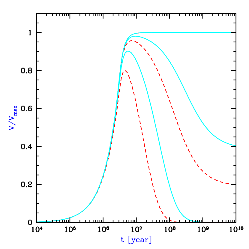
Figure 21: Expanding H 2 region around an isolated ionizing source. The comoving ionized volume $V$ is expressed in units of the maximum possible volume, $V_{\rm max}=4\pi r_{\rm max}^{3}/3$ [with $r_{\rm max}$ given in equation (73)], and the time is measured after an instantaneous starburst which produces ionizing photons according to equation (74). We consider a source turning on at $z=10$ (solid curves) or $z=15$ (dashed curves), with three cases for each: no recombinations, $C=1$, and $C=10$, in order from top to bottom. The no-recombination curve is identical for the different source redshifts.

We obtain a similar result for the size of the H 2 region around a galaxy if we consider a mini-quasar rather than stars. For the typical quasar spectrum (Elvis et al. 1994), if we assume a radiative efficiency of $\sim 6\%$ then roughly 11,000 ionizing photons are produced per baryon incorporated into the black hole (Haiman, personal communication). The efficiency of incorporating the baryons in a galaxy into a central black hole is low ($\lesssim 0.6\%$ in the local universe, e.g. Magorrian et al. 1998; see also §8.2.2), but the escape fraction for quasars is likely to be close to unity, i.e., an order of magnitude higher than for stars (see §6.1). Thus, for every baryon in galaxies, up to $\sim 65$ ionizing photons may be produced by a central black hole and $\sim 40$ by stars, although both of these numbers for $N_{\rm ion}$ are highly uncertain. These numbers suggest that in either case the typical size of H 2 regions before reionization may be $\lesssim 1$ Mpc or $\sim 10$ Mpc, depending on whether $10^{8}M_{\sun}$ halos or $10^{12}M_{\sun}$ halos dominate.

6.3 Reionization of the IGM

6.3.1 Hydrogen Reionization

In this section we summarize recent progress, both analytic and numerical, made toward elucidating the basic physics of reionization and the way in which the characteristics of reionization depend on the nature of the ionizing sources and on other input parameters of cosmological models.

The process of the reionization of hydrogen involves several distinct stages. The initial, “pre-overlap” stage (using the terminology of Gnedin 2000a) consists of individual ionizing sources turning on and ionizing their surroundings. The first galaxies form in the most massive halos at high redshift, and these halos are biased and are preferentially located in the highest-density regions. Thus the ionizing photons which escape from the galaxy itself (see §6.1) must then make their way through the surrounding high-density regions, which are characterized by a high recombination rate. Once they emerge, the ionization fronts propagate more easily into the low-density voids, leaving behind pockets of neutral, high-density gas. During this period the IGM is a two-phase medium characterized by highly ionized regions separated from neutral regions by ionization fronts. Furthermore, the ionizing intensity is very inhomogeneous even within the ionized regions, with the intensity determined by the distance from the nearest source and by the ionizing luminosity of this source.

The central, relatively rapid “overlap” phase of reionization begins when neighboring H 2 regions begin to overlap. Whenever two ionized bubbles are joined, each point inside their common boundary becomes exposed to ionizing photons from both sources. Therefore, the ionizing intensity inside H 2 regions rises rapidly, allowing those regions to expand into high-density gas which had previously recombined fast enough to remain neutral when the ionizing intensity had been low. Since each bubble coalescence accelerates the process of reionization, the overlap phase has the character of a phase transition and is expected to occur rapidly, over less than a Hubble time at the overlap redshift. By the end of this stage most regions in the IGM are able to see several unobscured sources, and therefore the ionizing intensity is much higher than before overlap and it is also much more homogeneous. An additional ingredient in the rapid overlap phase results from the fact that hierarchical structure formation models predict a galaxy formation rate that rises rapidly with time at the relevant redshift range. This process leads to a state in which the low-density IGM has been highly ionized and ionizing radiation reaches everywhere except for gas located inside self-shielded, high-density clouds. This marks the end of the overlap phase, and this important landmark is most often referred to as the ’moment of reionization’.

Some neutral gas does, however, remain in high-density structures which correspond to Lyman Limit systems and damped Ly$\alpha$ systems seen in absorption at lower redshifts. The high-density regions are gradually ionized as galaxy formation proceeds, and the mean ionizing intensity also grows with time. The ionizing intensity continues to grow and to become more uniform as an increasing number of ionizing sources is visible to every point in the IGM. This “post-overlap” phase continues indefinitely, since collapsed objects retain neutral gas even in the present universe. The IGM does, however, reach another milestone (of limited significance) at $z\sim 1.6$, the breakthrough redshift (which is determined by the probability of intersecting Lyman limit systems; Madau, Haardt, & Rees 1999). Below this redshift, all ionizing sources are visible to each other, while above this redshift absorption by the Ly$\alpha$ forest clouds implies that only sources in a small redshift range are visible to a typical point in the IGM.

Semi-analytic models of the pre-overlap stage focus on the evolution of the H 2 filling factor, i.e., the fraction of the volume of the universe which is filled by H 2 regions. We distinguish between the naive filling factor $F_{\rm H\ II}$ and the actual filling factor or porosity $Q_{\rm H\ II}$. The naive filling factor equals the number density of bubbles times the average volume of each, and it may exceed unity since when bubbles begin to overlap the overlapping volume is counted multiple times. However, as explained below, in the case of reionization the linearity of the physics means that $F_{\rm H\ II}$ is a very good approximation to $Q_{\rm H\ II}$ up to the end of the overlap phase of reionization.

The model of individual H 2 regions presented in the previous section can be used to understand the development of the total filling factor. Starting with equation (65), if we assume a common clumping factor $C$ for all H 2 regions then we can sum each term of the equation over all bubbles in a given large volume of the universe, and then divide by this volume. Then $V$ is replaced by the filling factor and $N_{\gamma}$ by the total number of ionizing photons produced up to some time $t$, per unit volume. The latter quantity equals the mean number of ionizing photons per baryon times the mean density of baryons $\bar{n}_{b}$. Following the arguments leading to equation (73), we find that if we include only stars then

$$\frac{\bar{n}_{\gamma}}{\bar{n}_{b}}=N_{\rm ion}F_{\rm col}\ ,$$ (75)

where the collapse fraction $F_{\rm col}$ is the fraction of all the baryons in the universe which are in galaxies, i.e., the fraction of gas which settles into halos and cools efficiently inside them. In writing equation (75) we are assuming instantaneous production of photons, i.e., that the time-scale for the formation and evolution of the massive stars in a galaxy is short compared to the Hubble time at the formation redshift of the galaxy. In a model based on equation (65), the near-equality between $F_{\rm H\ II}$ and $Q_{\rm H\ II}$ results from the linearity of this equation. First, the total number of ionizations equals the total number of ionizing photons produced by stars, i.e., all ionizing photons contribute regardless of the spatial distribution of sources; and second, the total recombination rate is proportional to the total ionized volume, regardless of its topology. Thus, even if two or more bubbles overlap the model remains an accurate approximation for $Q_{\rm H\ II}$ (at least until $Q_{\rm H\ II}$ becomes nearly equal to 1). Note, however, that there still are a number of important simplifications in the model, including the assumption of a homogeneous (though possibly time-dependent) clumping factor, and the neglect of feedback whereby the formation of one galaxy may suppress further galaxy formation in neighboring regions. These complications are discussed in detail below and in §6.5 and §7.

Under these assumptions we convert equation (65), which describes individual H 2 regions, to an equation which statistically describes the transition from a neutral universe to a fully ionized one (compare Madau et al. 1999 and Haiman & Loeb 1997):

$$\frac{dQ_{\rm H\ II}}{dt}=\frac{N_{\rm ion}}{0.76}\frac{dF_{\rm col}}{dt}-\alpha_{B}\frac{C}{a^{3}}\bar{n}_{H}^{0}Q_{\rm H\ II}\ ,$$ (76)

where we assumed a primordial mass fraction of hydrogen of 0.76. The solution (in analogy with equation (67)) is

$$Q_{\rm H\ II}(t)=\int_{0}^{t}\frac{N_{\rm ion}}{0.76}\frac{dF_{\rm col}}{dt^{\prime}}\,e^{F(t^{\prime},t)}dt^{\prime}\ ,$$ (77)

where $F(t^{\prime},t)$ is determined by equations (68)–(71).

A simple estimate of the collapse fraction at high redshift is the mass fraction (given by equation (31) in the Press-Schechter model) in halos above the cooling threshold, which is the minimum mass of halos in which gas can cool efficiently. Assuming that only atomic cooling is effective during the redshift range of reionization (§3.3), the minimum mass corresponds roughly to a halo of virial temperature $T_{\rm vir}=10^{4}$ K, which can be converted to a mass using equation (26). With this prescription we derive (for $N_{\rm ion}=40$) the reionization history shown in Figure 22 for the case of a constant clumping factor $C$. The solid curves show $Q_{\rm H\ II}$ as a function of redshift for a clumping factor $C=0$ (no recombinations), $C=1$, $C=10$, and $C=30$, in order from left to right. Note that if $C\sim 1$ then recombinations are unimportant, but if $C\gtrsim 10$ then recombinations significantly delay the reionization redshift (for a fixed star-formation history). The dashed curve shows the collapse fraction $F_{\rm col}$ in this model. For comparison, the vertical dotted line shows the $z=5.8$ observational lower limit (Fan et al. 2000) on the reionization redshift.

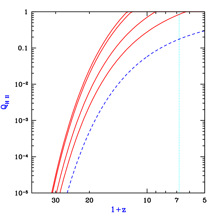
Figure 22: Semi-analytic calculation of the reionization of the IGM (for $N_{\rm ion}=40$), showing the redshift evolution of the filling factor $Q_{\rm H\ II}$. Solid curves show $Q_{\rm H\ II}$ for a clumping factor $C=0$ (no recombinations), $C=1$, $C=10$, and $C=30$, in order from left to right. The dashed curve shows the collapse fraction $F_{\rm col}$, and the vertical dotted line shows the $z=5.8$ observational lower limit (Fan et al. 2000) on the reionization redshift.

Clearly, star-forming galaxies in CDM hierarchical models are capable of ionizing the universe at $z\sim 6$–15 with reasonable parameter choices. This has been shown by a number of theoretical, semi-analytic calculations (Fukugita & Kawasaki 1994; Shapiro, Giroux, & Babul 1994; Kamionkowski, Spergel, & Sugiyama 1994; Tegmark, Silk, & Blanchard 1994; Haiman & Loeb 1997; Valageas & Silk 1999; Chiu & Ostriker 2000; Ciardi et al. 2000) as well as numerical simulations (Cen & Ostriker 1993; Gnedin & Ostriker 1997; Gnedin 2000a). Similarly, if a small fraction ($\lesssim 1\%$) of the gas in each galaxy accretes onto a central black hole, then the resulting mini-quasars are also able to reionize the universe, as has also been shown using semi-analytic models (Fukugita & Kawasaki 1994; Haiman & Loeb 1998; Valageas & Silk 1999). Note that the prescription whereby a constant fraction of the galactic mass accretes onto a central black hole is based on local observations (see §8.2.2) which indicate that $z=0$ galaxies harbor central black holes of mass equal to $\sim 0.2$–$0.6\%$ of their bulge mass. Although the bulge constitutes only a fraction of the total baryonic mass of each galaxy, the higher gas-to-stellar mass ratio in high-redshift galaxies, as well as their high merger rates compared to their low-redshift counterparts, suggest that a fraction of a percent of the total gas mass in high-redshift galaxies may have contributed to the formation of quasar black holes.

Although many models yield a reionization redshift around 7–12, the exact value depends on a number of uncertain parameters affecting both the source term and the recombination term in equation (76). The source parameters include the formation efficiency of stars and quasars and the escape fraction of ionizing photons produced by these sources. The formation efficiency of low-mass galaxies may also be reduced by feedback from galactic outflows. These parameters affecting the sources are discussed elsewhere in this review (see §5.2, 8.2.2, 6.1, and 7). Even when the clumping is inhomogeneous, the recombination term in equation (76) is generally valid if $C$ is defined as in equation (64), where we take a global volume average of the square of the density inside ionized regions (since neutral regions do not contribute to the recombination rate). The resulting mean clumping factor depends on the density and clustering of sources, and on the distribution and topology of density fluctuations in the IGM. Furthermore, the source halos should tend to form in overdense regions, and the clumping factor is affected by this cross-correlation between the sources and the IGM density.

Valageas & Silk (1999) and Chiu & Ostriker (2000) calculated the clumping factor semi-analytically by averaging over the IGM on the one hand and virialized halos on the other hand, with the average weighed according to the gas fraction in halos. The semi-analytic methods used in these two detailed calculations of reionization have different advantages: Valageas & Silk (1999) included a model for clumping and absorption by Ly$\alpha$ clouds, but Chiu & Ostriker (2000) used a generally more realistic two-phase model with separate ionized and neutral regions. Miralda-Escudé, Haehnelt, & Rees (2000) went further in their modeling of the clumping factor by attempting to account for the geometry of ionized regions. They presented a simple model for the distribution of density fluctuations, and more generally they discussed the implications of inhomogeneous clumping during reionization. They noted that as ionized regions grow, they more easily extend into low-density regions, and they tend to leave behind high-density concentrations, with these neutral islands being ionized only at a later time. They therefore argued that, since at high-redshift the collapse fraction is low, most of the high-density regions, which would dominate the clumping factor if they were ionized, will in fact remain neutral and occupy only a tiny fraction of the total volume. Thus, the development of reionization through the end of the overlap phase should occur almost exclusively in the low-density IGM, and the effective clumping factor during this time should be $\sim 1$, making recombinations relatively unimportant (see Figure 22). Only in the post-reionization phase, Miralda-Escudé et al. (2000) argued, do the high density clouds and filaments become gradually ionized as the mean ionizing intensity further increases.

The complexity of the process of reionization is illustrated by the recent numerical simulation by Gnedin (2000a) of stellar reionization (in $\Lambda$CDM with ${\Omega_{m}}=0.3$). This simulation uses a formulation of radiative transfer which relies on several rough approximations; although it does not include the effect of shadowing behind optically-thick clumps, it does include for each point in the IGM the effects of an estimated local optical depth around that point, plus a local optical depth around each ionizing source. This simulation helps to understand the advantages of the various theoretical approaches, while pointing to the complications which are not included in the simple models. Figures 23 and 24, taken from Figure 3 in Gnedin (2000a), show the state of the simulated universe just before and just after the overlap phase, respectively. They show a thin (15 $h^{-1}$ comoving kpc) slice through the box, which is 4 $h^{-1}$ Mpc on a side. The simulation achieves a spatial resolution of $1h^{-1}$ kpc, and uses $128^{3}$ each of dark matter particles and baryonic particles (with each baryonic particle having a mass of $5\times 10^{5}M_{\sun}$). The figures show the redshift evolution of the ionizing intensity averaged over the entire volume, $J_{21}$ (upper right panel), and, visually, the spatial distribution of three quantities: the neutral hydrogen fraction (upper left panel), the gas density (lower left panel), and the gas temperature (lower right panel). Note the obvious features around the edges, resulting from the periodic boundary conditions assumed in the simulation (e.g., the left and right edges match identically). Also note that the intensity $J_{21}$ is defined as the radiation intensity at the Lyman limit, expressed in units of $10^{-21}\,\mbox{ erg cm}^{-2}\mbox{ s}^{-1}\mbox{ sr}^{-1}\mbox{Hz}^{-1}$. For a given source emission, the intensity inside H 2 regions depends on absorption and radiative transfer through the IGM (e.g., Haardt & Madau 1996; Abel & Haehnelt 1999)

Figure 23 shows the two-phase IGM at $z=7.7$, with ionized bubbles emanating from many independent sources, although there is one main concentration (located at the right edge of the image, vertically near the center; note the periodic boundary conditions). The bubbles are shown expanding into low density regions and beginning to overlap at the center of the image. The topology of ionized regions is clearly complex: While the ionized regions are analogous to islands in an ocean of neutral hydrogen, the islands themselves contain small lakes of dense neutral gas. One aspect which has not been included in theoretical models of clumping is clear from the figure. The sources themselves are located in the highest density regions (these being the sites where the earliest galaxies form) and must therefore ionize the gas in their immediate vicinity before the radiation can escape into the low density IGM. For this reason, the effective clumping factor is of order 100 in the simulation and also, by the overlap redshift, roughly ten ionizing photons have been produced per baryon. As emphasized by Gnedin (2000a), some of these numbers are resolution dependent, since the clumping factor accounts only for absorption by gas at the highest resolvable density. A higher-resolution simulation would have higher-density gas clumps and — depending on the geometry of those clumps — a higher or possibly lower clumping factor than the low-resolution simulation. Figure 24 shows that by $z=6.7$ the low density regions have all become highly ionized along with a rapid increase in the ionizing intensity. The only neutral islands left are the highest density regions which are not near the sources (compare the two panels on the left). However, we emphasize that the quantitative results of this simulation must be considered preliminary, since the effects of increased resolution and a more accurate treatment of radiative transfer are yet to be explored. Methods are being developed for incorporating a more complete treatment of radiative transfer into three dimensional cosmological simulations (e.g., Abel, Norman, & Madau 1999; Razoumov & Scott 1999).

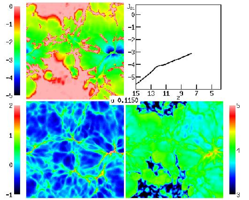
Figure 23: Visualization at $z=7.7$ of a numerical simulation of reionization, adopted from Figure 3c of Gnedin (2000a). The panels display the logarithm of the neutral hydrogen fraction (upper left), the gas density in units of the cosmological mean (lower left), and the gas temperature in Kelvin (lower right). These panels show a two-dimensional slice of the simulation (not a two-dimensional projection). Also shown is the redshift evolution of the logarithm of the ionizing intensity averaged over the entire simulation volume (upper right). Note the periodic boundary conditions.

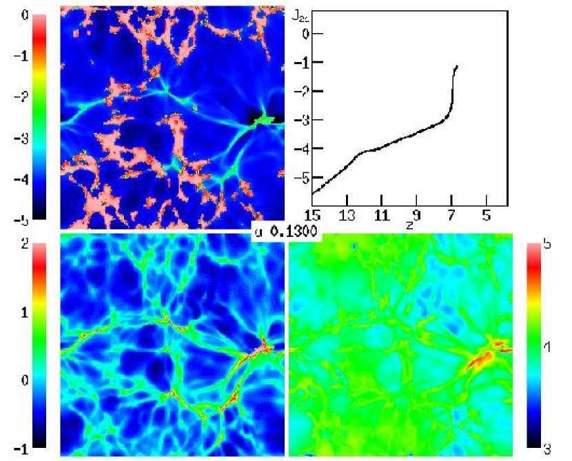
Figure 24: Visualization at $z=6.7$ of a numerical simulation of reionization, adopted from Figure 3c of Gnedin (2000a). The panels display the logarithm of the neutral hydrogen fraction (upper left), the gas density in units of the cosmological mean (lower left), and the gas temperature in Kelvin (lower right). These panels show a two-dimensional slice of the simulation (not a two-dimensional projection). Also shown is the redshift evolution of the logarithm of the ionizing intensity averaged over the entire simulation volume (upper right). Note the periodic boundary conditions.

Gnedin, Ferrara, & Zweibel (2000) investigated an additional effect of reionization. They showed that the Biermann battery in cosmological ionization fronts inevitably generates coherent magnetic fields of an amplitude $\sim 10^{-19}$ Gauss. These fields form as a result of the breakout of the ionization fronts from galaxies and their propagation through the H 1 filaments in the IGM. Although the fields are too small to directly affect galaxy formation, they could be the seeds for the magnetic fields observed in galaxies and X-ray clusters today.

If quasars contribute substantially to the ionizing intensity during reionization then several aspects of reionization are modified compared to the case of pure stellar reionization. First, the ionizing radiation emanates from a single, bright point-source inside each host galaxy, and can establish an escape route (H 2 funnel) more easily than in the case of stars which are smoothly distributed throughout the galaxy (§6.1). Second, the hard photons produced by a quasar penetrate deeper into the surrounding neutral gas, yielding a thicker ionization front. Finally, the quasar X-rays catalyze the formation of H₂ molecules and allow stars to keep forming in very small halos (§3.3).

Oh (2000) showed that star-forming regions may also produce significant X-rays at high redshift. The emission is due to inverse Compton scattering of CMB photons off relativistic electrons in the ejecta, as well as thermal emission by the hot supernova remnant. The spectrum expected from this process is even harder than for typical quasars, and the hard photons photoionize the IGM efficiently by repeated secondary ionizations. The radiation, characterized by roughly equal energy per logarithmic frequency interval, would produce a uniform ionizing intensity and lead to gradual ionization and heating of the entire IGM. Thus, if this source of emission is indeed effective at high redshift, it may have a crucial impact in changing the topology of reionization. Even if stars dominate the emission, the hardness of the ionizing spectrum depends on the initial mass function. At high redshift it may be biased toward massive, efficiently ionizing stars (see §4.1.1), but this remains very much uncertain.

Semi-analytic as well as numerical models of reionization depend on an extrapolation of hierarchical models to higher redshifts and lower-mass halos than the regime where the models have been compared to observations. These models have the advantage that they are based on the current CDM paradigm which is supported by a variety of observations of large-scale structure, galaxy clustering, and the CMB. The disadvantage is that the properties of high-redshift galaxies are derived from those of their host halos by prescriptions which are based on low-redshift observations, and these prescriptions will only be tested once abundant data is available on galaxies which formed during the reionization era. An alternative approach to analyzing the possible ionizing sources which brought about reionization is to extrapolate from the observed populations of galaxies and quasars at currently accessible redshifts. This has been attempted, e.g., by Madau et al. (1999) and Miralda-Escudé et al. (2000). The general conclusion is that a high-redshift source population similar to the one observed at $z=3$–4 would produce roughly the needed ionizing intensity for reionization. A precise conclusion, however, remains elusive because of the same kinds of uncertainties as those found in the models based on CDM: The typical escape fraction, and the faint end of the luminosity function, are both not well determined even at $z=3$–4, and in addition the clumping factor at high redshift must be known in order to determine the importance of recombinations. Future direct observations of the source population at redshifts approaching reionization may help resolve some of these questions.

6.3.2 Helium Reionization

The sources that reionized hydrogen very likely caused the single reionization of helium from He 1 to He 2. Neutral helium is ionized by photons of 24.6 eV or higher energy, and its recombination rate is roughly equal to that of hydrogen. On the other hand, the ionization threshold of He 2 is 54.4 eV, and fully ionized helium recombines $\gtrsim 5$ times faster than hydrogen. This means that for both quasars and galaxies, the reionization of He 2 should occur later than the reionization of hydrogen, even though the number of helium atoms is smaller than hydrogen by a factor of 13. The lower redshift of He 2 reionization makes it more accessible to observations and allows it to serve in some ways as an observational preview of hydrogen reionization.

The Ly$\alpha$ absorption by intergalactic He 2 (at wavelength $304$Å) has been observed in four quasars at redshifts $2.4<z<3.2$ (Jakobsen et al. 1994; Davidsen et al. 1996; Hogan et al. 1997; Reimers et al. 1997; Anderson et al. 1999; Heap et al. 2000). The results are consistent among the different quasars, and we illustrate them here with one particular spectrum. In Figure 25, adopted from Figure 4 of Heap et al. (2000), we show a portion of the spectrum of the $z=3.286$ quasar $Q\ 0302-003$, obtained with the Space Telescope Imaging Spectrograph on-board the Hubble Space Telescope.  The observed spectrum (solid line) is compared to a simulated spectrum (gray shading) based on the H 1 Ly$\alpha$ forest observed in the same quasar. In deriving the simulated spectrum, Heap et al. assumed a ratio of He 2 to H 1 column densities of 100, and pure turbulent line broadening. The wavelength range shown in the figure corresponds to He 2 Ly$\alpha$ in the redshift range 2.8–3.3.

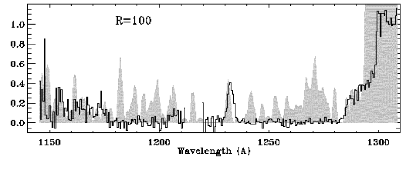
Figure 25: Ly$\alpha$ absorption by intergalactic He 2. This spectrum of the $z=3.286$ quasar $Q\ 0302-003$, adopted from Figure 4 of Heap et al. (2000), was obtained using the Space Telescope Imaging Spectrograph. The observed spectrum (solid line) is compared to a simulated spectrum (gray shading) based on the H 1 Ly$\alpha$ forest observed in the same quasar. In deriving the simulated spectrum, Heap et al. assumed a ratio of He 2 to H 1 column densities of 100, and pure turbulent line broadening.

The observed flux shows a clear break shortward of the quasar emission line at an observed $\lambda=1300$ Å. Relatively near the quasar, at $\lambda=$1285–1300Å, a shelf of relatively high transmission is likely evidence of the ’proximity effect’, in which the emission from the quasar itself creates a highly ionized local region with a reduced abundance of absorbing ions. In the region at $\lambda=$1240–1280 Å ($z=3.08$–3.21), on the other hand, the very low flux level implies an average optical depth of $\tau\sim 4.5$–5 due to He 2. Another large region with average $\tau\sim 4$, a region spanning $\sim 100$ comoving Mpc along the line of sight, is evident at $\lambda=$1180–1210Å ($z=2.88$–2.98). The strong continuous absorption in these large regions, and the lack of correlation with the observed H 1 Ly$\alpha$ forest, is evidence for a He 2 Gunn-Peterson absorption trough due to the diffuse IGM. It also suggests a rather soft UV background with a significant stellar contribution, i.e., a background that ionizes the diffuse hydrogen much more thoroughly than He 2. Significant emission is observed in between the two regions of constant high absorption. A small region around 1216Å is contaminated by geo-coronal Ly$\alpha$, but the emission at 1230–1235Å apparently corresponds to a real, distinct gap in the He 2 abundance, which could be caused by a local source photo-ionizing a region of radius $\sim 10$ comoving Mpc. The region at $\lambda=$1150–1175Å  ($z=2.78$–2.86) shows a much higher overall transmission level than the regions at slightly higher redshift. Heap et al. measure an average $\tau=1.9$ in this region, and note that the significant correlation of the observed spectrum with the simulated one suggests that much of the absorption is due to a He 2 Ly$\alpha$ forest while the low-density IGM provides a relatively low opacity in this region. The authors conclude that the observed data suggest a sharp opacity break occurring between $z=3.0$ and 2.9, accompanied by a hardening of the UV ionizing background. However, even the relatively high opacity at $z\gtrsim 3$ only requires $\sim 0.1\%$ of helium atoms not to be fully ionized, in a region at the mean baryon density. Thus, the overlap phase of full helium reionization may have occurred significantly earlier, with the ionizing intensity already fairly uniform but still increasing with time at $z\sim 3$.

The properties of helium reionization have been investigated numerically by a number of authors. Zheng & Davidsen (1995) modeled the He 2 proximity effect, and a number of authors (Miralda-Escudé et al. 1996; Croft et al. 1997; Zhang et al. 1998) used numerical simulations to show that the observations generally agree with cold dark matter models. They also found that helium absorption particularly tests the properties of under-dense voids which produce much of the He 2 opacity but little opacity in H 1. According to the semi-analytic model of inhomogeneous reionization of Miralda-Escudé, Haehnelt, & Rees (2000; see also §6.3.1), the total emissivity of observed quasars at redshift 3 suffices to completely reionize helium before $z=3$. They find that the observations at $z\sim 3$ can be reproduced if a population of low-luminosity sources, perhaps galaxies, has ionized the low-density IGM up to an overdensity of around 12 relative to the cosmological mean, with luminous quasars creating the observed gaps of transmitted flux.

The conclusion that an evolution of the ionization state of helium has been observed is also strengthened by several indirect lines of evidence. Songaila & Cowie (1996) and Songaila (1998) found a rapid increase in the Si 4/C 4 ratio with decreasing redshift at $z=3$, for intermediate column density hydrogen Ly$\alpha$ absorption lines. They interpreted this evolution as a sudden hardening below $z=3$ of the spectrum of the ionizing background. Boksenberg et al. (1998) also found an increase in the Si 4/C 4 ratio, but their data implied a much more gradual increase from $z=3.8$ to $z=2.2$.

The full reionization of helium due to a hard ionizing spectrum should also heat the IGM to 20,000 K or higher, while the IGM can only reach $\sim$10,000 K during a reionization of hydrogen alone (although a temperature of $\sim$15,000 K may be reached due to Compton heating by the hard X-ray background: Madau & Efstathiou 1999). This increase in temperature can serve as an observational probe of helium reionization, and it should also increase the suppression of dwarf galaxy formation (§6.5). The temperature of the IGM can be measured by searching for the smallest line-widths among hydrogen Ly$\alpha$ absorption lines (Schaye et al. 1999). In general, bulk velocity gradients contribute to the line width on top of thermal velocities, but a lower bound on the width is set by thermal broadening, and the narrowest lines can be used to measure the temperature. Several different measurements (Ricotti et al. 2000; Schaye et al. 2000; Bryan & Machacek 2000; McDonald et al. 2000) have found a nearly isothermal IGM at a temperature of $\sim$20,000 K at $z=3$, higher than expected in ionization equilibrium and suggestive of photo-heating due to ongoing reionization of helium. However, the measurement errors remain too large for a firm conclusion about the redshift evolution of the IGM temperature or its equation of state.

Clearly, the reionization of helium is already a rich phenomenological subject. Our knowledge will benefit from measurements of increasing accuracy, made toward many more lines of sight, and extended to higher redshift. New ways to probe helium will also be useful. For example, Miralda-Escudé (2000) has suggested that continuum He 2 absorption in soft X-rays can be used to determine the He 2 fraction along the line of sight, although the measurement requires an accurate subtraction of the Galactic contribution to the absorption, based on the Galactic H 1 column density as determined by 21 cm maps.

6.4 Photo-evaporation of Gaseous Halos After Reionization

The end of the reionization phase transition resulted in the emergence of an intense UV background that filled the universe and heated the IGM to temperatures of $\sim 1$–$2\times 10^{4}$K (see the previous section). After ionizing the rarefied IGM in the voids and filaments on large scales, the cosmic UV background penetrated the denser regions associated with the virialized gaseous halos of the first generation of objects. A major fraction of the collapsed gas had been incorporated by that time into halos with a virial temperature $\lesssim 10^{4}$K, where the lack of atomic cooling prevented the formation of galactic disks and stars or quasars. Photoionization heating by the cosmic UV background could then evaporate much of this gas back into the IGM. The photo-evaporating halos, as well as those halos which did retain their gas, may have had a number of important consequences just after reionization as well as at lower redshifts.

In this section we focus on the process by which gas that had already settled into virialized halos by the time of reionization was evaporated back into the IGM due to the cosmic UV background. This process was investigated by Barkana & Loeb (1999) using semi-analytic methods and idealized numerical calculations. They first considered an isolated spherical, centrally-concentrated dark matter halo containing gas. Since most of the photo-evaporation occurs at the end of overlap, when the ionizing intensity builds up almost instantaneously, a sudden illumination by an external ionizing background may be assumed. Self-shielding of the gas implies that the halo interior sees a reduced intensity and a harder spectrum, since the outer gas layers preferentially block photons with energies just above the Lyman limit. It is useful to parameterize the external radiation field by a specific intensity per unit frequency, $\nu$,

$$J_{\nu}=10^{-21}\,J_{21}\,\left(\frac{\nu}{\nu_{L}}\right)^{-\alpha}\mbox{ erg cm}^{-2}\mbox{ s}^{-1}\mbox{ sr}^{-1}\mbox{Hz}^{-1}\ ,$$ (78)

where $\nu_{L}$ is the Lyman limit frequency, and $J_{21}$ is the intensity at $\nu_{L}$ expressed in units of $10^{-21}\,\mbox{ erg cm}^{-2}\mbox{ s}^{-1}\mbox{ sr}^{-1}\mbox{Hz}^{-1}$. The intensity is normalized to an expected post-reionization value of around unity for the ratio of ionizing photon density to the baryon density. Different power laws can be used to represent either quasar spectra ($\alpha\sim 1.8$) or stellar spectra ($\alpha\sim 5$).

Once the gas is heated throughout the halo, some fraction of it acquires a sufficiently high temperature that it becomes unbound. This gas expands due to the resulting pressure gradient and eventually evaporates back into the IGM. The pressure gradient force (per unit volume) $k_{\rm B}\nabla(T\rho/\mu m_{p})$ competes with the gravitational force of $\rho\,GM/r^{2}$. Due to the density gradient, the ratio between the pressure force and the gravitational force is roughly equal to the ratio between the thermal energy $\sim k_{\rm B}T$ and the gravitational binding energy $\sim\mu m_{p}GM/r$ (which is $\sim k_{\rm B}T_{\rm vir}$ at the virial radius $r_{\rm vir}$) per particle. Thus, if the kinetic energy exceeds the potential energy (or roughly if $T>T_{\rm vir}$), the repulsive pressure gradient force exceeds the attractive gravitational force and expels the gas on a dynamical time (or faster for halos with $T\gg T_{\rm vir}$).

The left panel of Figure 26 (adopted from Figure 3 of Barkana & Loeb 1999) shows the fraction of gas within the virial radius which becomes unbound after reionization, as a function of the total halo circular velocity, with halo masses at $z=8$ indicated at the top. The two pairs of curves correspond to spectral index $\alpha=5$ (solid) or $\alpha=1.8$ (dashed). In each pair, a calculation which assumes an optically-thin halo leads to the upper curve, but including radiative transfer and self-shielding modifies the result to the one shown by the lower curve. In each case self-shielding lowers the unbound fraction, but it mostly affects only a neutral core containing $\sim 30\%$ of the gas. Since high energy photons above the Lyman limit penetrate deep into the halo and heat the gas efficiently, a flattening of the spectral slope from $\alpha=5$ to $\alpha=1.8$ raises the unbound gas fraction. This Figure is essentially independent of redshift if plotted in terms of circular velocity, but the conversion to a corresponding mass does vary with redshift. The characteristic circular velocity where most of the gas is lost is $\sim 10$–$15~{}{\rm km~{}s^{-1}}$, but clearly the effect of photo-evaporation is gradual, going from total gas removal down to no effect over a range of a factor of $\sim 100$ in halo mass.

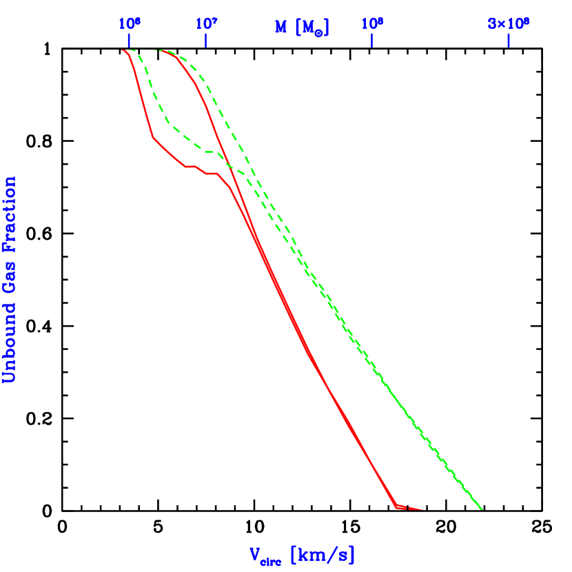
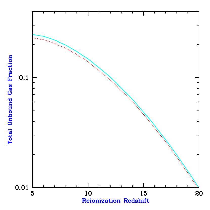
Figure 26: Effect of photo-evaporation on individual halos and on the overall halo population. The left panel shows the unbound gas fraction (within the virial radius) versus total halo circular velocity or mass, adopted from Figure 3 of Barkana & Loeb (1999). The two pairs of curves correspond to spectral index $\alpha=5$ (solid) or $\alpha=1.8$ (dashed), in each case at $z=8$. In each pair, assuming an optically-thin halo leads to the upper curve, while the lower curve shows the result of including radiative transfer and self shielding. The right panel shows the total fraction of gas in the universe which evaporates from halos at reionization, versus the reionization redshift, adopted from Figure 7 of Barkana & Loeb (1999). The solid line assumes a spectral index $\alpha=1.8$, and the dotted line assumes $\alpha=5$.

Given the values of the unbound gas fraction in halos of different masses, the Press-Schechter mass function (§2.4) can be used to calculate the total fraction of the IGM which goes through the process of accreting onto a halo and then being recycled into the IGM at reionization. The low-mass cutoff in this sum over halos is given by the lowest mass halo in which gas has assembled by the reionization redshift. This mass can be estimated by the linear Jeans mass $M_{\rm J}$ in equation (41) in §3.1. The Jeans mass does not in general precisely equal the limiting mass for accretion (see the discussion in the next section). Indeed, at a given redshift some gas can continue to fall into halos of lower mass than the Jeans mass at that redshift. On the other hand, the larger Jeans mass at higher redshifts means that a time-averaged Jeans mass may be more appropriate, as indicated by the filtering mass. In practice, the Jeans mass is sufficiently accurate since at $z\sim 10$–20 it agrees well with the values found in the numerical spherical collapse calculations of Haiman, Thoul, & Loeb (1996).

The right panel of Figure 26 (adopted from Figure 7 of Barkana & Loeb 1999) shows the total fraction of gas in the universe which evaporates from halos at reionization, versus the reionization redshift. The solid line assumes a spectral index $\alpha=1.8$, and the dotted line assumes $\alpha=5$, showing that the result is insensitive to the spectrum. Even at high redshift, the amount of gas which participates in photo-evaporation is significant, which suggests a number of possible implications as discussed below. The gas fraction shown in the figure represents most ($\sim 60$–$80\%$ depending on the redshift) of the collapsed fraction before reionization, although some gas does remain in more massive halos.

The photo-evaporation of gas out of large numbers of halos may have interesting implications. First, gas which falls into halos and is expelled at reionization attains a different entropy than if it had stayed in the low-density IGM. The resulting overall reduction in the entropy is expected to be small — the same as would be produced by reducing the temperature of the entire IGM by a factor of $\sim 1.5$ — but localized effects near photo-evaporating halos may be more significant. Furthermore, the resulting $\sim 20~{}{\rm km~{}s^{-1}}$ outflows induce small-scale fluctuations in peculiar velocity and temperature. These outflows are usually well below the resolution limit of most numerical simulations, but some outflows were resolved in the simulation of Bryan et al. (1998). The evaporating halos may consume a significant number of ionizing photons in the post-overlap stage of reionization (e.g., Haiman, Abel, & Madau 2000), but a definitive determination requires detailed simulations which include the three-dimensional geometry of source halos and sink halos.

Although gas is quickly expelled out of the smallest halos, photo-evaporation occurs more gradually in larger halos which retain some of their gas. These surviving halos initially expand but they continue to accrete dark matter and to merge with other halos. These evaporating gas halos could contribute to the high column density end of the Ly$\alpha$ forest (Bond, Szalay, & Silk 1988). Abel & Mo (1998) suggested that, based on the expected number of surviving halos, a large fraction of the Lyman limit systems at $z\sim 3$ may correspond to mini-halos that survived reionization. Surviving halos may even have identifiable remnants in the present universe, as discussed in §9.3. These ideas thus offer the possibility that a population of halos which originally formed prior to reionization may correspond almost directly to several populations that are observed much later in the history of the universe. However, the detailed dynamics of photo-evaporating halos are complex, and detailed simulations are required to confirm these ideas. Photo-evaporation of a gas cloud has been followed in a two dimensional simulation with radiative transfer, by Shapiro & Raga (2000). They found that an evaporating halo would indeed appear in absorption as a damped Ly$\alpha$ system initially, and as a weaker absorption system subsequently. Future simulations will clarify the contribution to quasar absorption lines of the entire population of photo-evaporating halos.

6.5 Suppression of the Formation of Low Mass Galaxies

At the end of overlap, the cosmic ionizing background increased sharply, and the IGM was heated by the ionizing radiation to a temperature $\gtrsim 10^{4}$ K. Due to the substantial increase in the IGM temperature, the intergalactic Jeans mass increased dramatically, changing the minimum mass of forming galaxies (Rees 1986; Efstathiou 1992; Gnedin & Ostriker 1997; Miralda-Escudé & Rees 1998).

Gas infall depends sensitively on the Jeans mass. When a halo more massive than the Jeans mass begins to form, the gravity of its dark matter overcomes the gas pressure. Even in halos below the Jeans mass, although the gas is initially held up by pressure, once the dark matter collapses its increased gravity pulls in some gas (Haiman, Thoul, & Loeb 1996). Thus, the Jeans mass is generally higher than the actual limiting mass for accretion. Before reionization, the IGM is cold and neutral, and the Jeans mass plays a secondary role in limiting galaxy formation compared to cooling. After reionization, the Jeans mass is increased by several orders of magnitude due to the photoionization heating of the IGM, and hence begins to play a dominant role in limiting the formation of stars. Gas infall in a reionized and heated universe has been investigated in a number of numerical simulations. Thoul & Weinberg (1996) inferred, based on a spherically-symmetric collapse simulation, a reduction of $\sim 50\%$ in the collapsed gas mass due to heating, for a halo of circular velocity $V_{c}\sim 50\ {\rm km\ s}^{-1}$ at $z=2$, and a complete suppression of infall below $V_{c}\sim 30\ {\rm km\ s}^{-1}$. Kitayama & Ikeuchi (2000) also performed spherically-symmetric simulations but included self-shielding of the gas, and found that it lowers the circular velocity thresholds by $\sim 5\ {\rm km\ s}^{-1}$. Three dimensional numerical simulations (Quinn, Katz, & Efstathiou 1996; Weinberg, Hernquist, & Katz 1997; Navarro & Steinmetz 1997) found a significant suppression of gas infall in even larger halos ($V_{c}\sim 75\ {\rm km\ s}^{-1}$), but this was mostly due to a suppression of late infall at $z\lesssim 2$.

When a volume of the IGM is ionized by stars, the gas is heated to a temperature $T_{\rm IGM}\sim 10^{4}$ K. If quasars dominate the UV background at reionization, their harder photon spectrum leads to $T_{\rm IGM}\sim 2\times 10^{4}$ K. Including the effects of dark matter, a given temperature results in a linear Jeans mass (see §3.1) corresponding to a halo circular velocity of

$$V_{J}=81\left(\frac{T_{\rm IGM}}{1.5\times 10^{4}{\rm K}}\right)^{1/2}\ \left[\frac{1}{{\Omega_{m}^{\,z}}}\ \frac{\Delta_{c}}{18\pi^{2}}\right]^{1/6}\ {\rm km\ s}^{-1},$$ (79)

where we used equation (25) and assumed $\mu=0.6$. In halos with $V_{c}>V_{J}$, the gas fraction in infalling gas equals the universal mean of $\Omega_{b}/{\Omega_{m}}$, but gas infall is suppressed in smaller halos. Even for a small dark matter halo, once it collapses to a virial overdensity of $\Delta_{c}/{\Omega_{m}^{\,z}}$ relative to the mean, it can pull in additional gas. A simple estimate of the limiting circular velocity, below which halos have essentially no gas infall, is obtained by substituting the virial overdensity for the mean density in the definition of the Jeans mass. The resulting estimate is

$$V_{\rm lim}=34\left(\frac{T_{\rm IGM}}{1.5\times 10^{4}{\rm K}}\right)^{1/2}\ {\rm km\ s}^{-1}.$$ (80)

This value is in rough agreement with the numerical simulations mentioned above (see also the related discussion in §3.2).

Although the Jeans mass is closely related to the rate of gas infall at a given time, it does not directly yield the total gas residing in halos at a given time. The latter quantity depends on the entire history of gas accretion onto halos, as well as on the merger histories of halos, and an accurate description must involve a time-averaged Jeans mass. Gnedin (2000b) showed that the gas content of halos in simulations is well fit by an expression which depends on the filtering mass, a particular time-averaged Jeans mass (Gnedin & Hui 1998; see also §3.1). Gnedin (2000b) calculated the Jeans and filtering masses using the mean temperature in the simulation to define the sound speed, and found the following fit to the simulation results:

$$\bar{M_{g}}=\frac{f_{b}M}{\left[1+\left(2^{1/3}-1\right)M_{C}/M\right]^{3}}\ ,$$ (81)

where $\bar{M_{g}}$ is the average gas mass of all objects with a total mass $M$, $f_{b}=\Omega_{b}/{\Omega_{m}}$ is the universal baryon fraction, and the characteristic mass $M_{C}$ is the total mass of objects which on average retain $50\%$ of their gas mass. The characteristic mass was well fit by the filtering mass at a range of redshifts from $z=4$ up to $z\sim 15$.

7 Feedback from Galactic Outflows

7.1 Propagation of Supernova Outflows in the IGM

Star formation is accompanied by the violent death of massive stars in supernova explosions. In general, if each halo has a fixed baryon fraction and a fixed fraction of the baryons turns into massive stars, then the total energy in supernova outflows is proportional to the halo mass. The binding energies of both the supernova ejecta and of all the gas in the halo are proportional to the halo mass squared. Thus, outflows are expected to escape more easily out of low-mass galaxies, and to expel a greater fraction of the gas from dwarf galaxies. At high redshifts, most galaxies form in relatively low-mass halos, and the high halo merger rate leads to vigorous star formation. Thus, outflows may have had a great impact on the earliest generations of galaxies, with consequences that may include metal enrichment of the IGM and the disruption of dwarf galaxies. In this subsection we present a simple model for the propagation of individual supernova shock fronts in the IGM. We discuss some implications of this model, but we defer to the following subsection the brunt of the discussion of the cosmological consequences of outflows.

For a galaxy forming in a given halo, the supernova rate is related to the star formation rate. In particular, for a Scalo (1998) initial stellar mass function, if we assume that a supernova is produced by each $M>8M_{\odot}$ star, then on average one supernova explodes for every 126 $M_{\odot}$ of star formation, expelling an ejecta mass of $\sim 3\,M_{\odot}$ including $\sim 1\,M_{\odot}$ of heavy elements. We assume that the individual supernovae produce expanding hot bubbles which merge into a single overall region delineated by an outwardly moving shock front. We assume that most of the baryons in the outflow lie in a thin shell, while most of the thermal energy is carried by the hot interior. The total ejected mass, which is lifted out of the halo by the outflow, equals a fraction $f_{\rm gas}$ of the total halo gas mass. The ejected mass includes some of the supernova ejecta itself. We let $f_{\rm eject}$ denote the fraction of the supernova ejecta that winds up in the outflow (with $f_{\rm eject}\leq 1$ since some metals may be deposited in the disk and not ejected). Since at high redshift most of the halo gas is likely to have cooled onto a disk, we assume that the mass carried by the outflow remains constant until the shock front reaches the halo virial radius. We assume an average supernova energy of $10^{51}E_{51}$ erg, a fraction $f_{\rm wind}$ of which remains in the outflow after the outflow escapes from the disk. The outflow must overcome the gravitational potential of the halo, which we assume to have a Navarro, Frenk, & White (1997) density profile [NFW; see equation (28) in §(2.3)]. Since the entire shell mass must be lifted out of the halo, we include the total shell mass as well as the total injected energy at the outset. This assumption is consistent with the fact that the burst of star formation in a halo is typically short compared to the total time for which the corresponding outflow expands.

The escape of an outflow from an NFW halo depends on the concentration parameter $c_{\rm N}$ of the halo. Simulations by Bullock et al. (2000) indicate that the concentration parameter decreases with redshift, and their results may be extrapolated to our regime of interest (i.e., to smaller halo masses and higher redshifts) by assuming that

$$c_{\rm N}=\left(\frac{M}{10^{9}M_{\sun}}\right)^{-0.1}\,\frac{25}{(1+z)}\ .$$ (82)

Although we calculate below the dynamics of each outflow in detail, it is also useful to estimate which halos can generate large-scale outflows by comparing the kinetic energy of the outflow to the potential energy needed to completely escape (i.e., to infinite distance) from an NFW halo. We thus find that the outflow can escape from its originating halo if the circular velocity is below a critical value given by

$$V_{\rm crit}=200\sqrt{\frac{E_{51}f_{\rm wind}(\eta/0.1)}{f_{\rm gas}\ g(c_{\rm N})}}\ {\rm km\ s}^{-1}\ ,$$ (83)

where the efficiency $\eta$ is the fraction of baryons incorporated in stars, and

$$g(x)=\frac{x^{2}}{(1+x)\ln(1+x)-x}\ .$$ (84)

Note that the contribution to $f_{\rm gas}$ of the supernova ejecta itself is $0.024\eta f_{\rm eject}$, so the ejecta mass is usually negligible unless $f_{\rm gas}\lesssim 1\%$. Equation (83) can also be used to yield the maximum gas fraction $f_{\rm gas}$ which can be ejected from halos, as a function of their circular velocity. Although this equation is most general, if we assume that the parameters $f_{\rm gas}$ and $f_{\rm wind}$ are independent of $M$ and $z$ then we can normalize them based on low-redshift observations. If we specify $c_{\rm N}\sim 10$ (with $g(10)=6.1$) at $z=0$, then setting $E_{51}=1$ and $\eta=10\%$ yields the required energy efficiency as a function of the ejected halo gas fraction:

$$f_{\rm wind}=1.5f_{\rm gas}\left[\frac{V_{\rm crit}}{100\ {\rm km\ s}^{-1}}\right]^{2}\ .$$ (85)

A value of $V_{\rm crit}\sim 100\ {\rm km\ s}^{-1}$ is suggested by several theoretical and observational arguments which are discussed in the next subsection. However, these arguments are not conclusive, and $V_{\rm crit}$ may differ from this value by a large factor, especially at high redshift (where outflows are observationally unconstrained at present). Note the degeneracy between $f_{\rm gas}$ and $f_{\rm wind}$ which remains even if $V_{\rm crit}$ is specified. Thus, if $V_{\rm crit}\sim 100\ {\rm km\ s}^{-1}$ then a high efficiency $f_{\rm wind}\sim 1$ is required to eject most of the gas from all halos with $V_{c}<V_{\rm crit}$, but only $f_{\rm wind}\sim 10\%$ is required to eject 5–10$\%$ of the gas. The evolution of the outflow does depend on the value of $f_{\rm wind}$ and not just the ratio $f_{\rm wind}/f_{\rm gas}$, since the shell accumulates material from the IGM which eventually dominates over the initial mass carried by the outflow.

We solve numerically for the spherical expansion of a galactic outflow, elaborating on the basic approach of Tegmark, Silk, & Evrard (1993). We assume that most of the mass $m$ carried along by the outflow lies in a thin, dense, relatively cool shell of proper radius $R$. The interior volume, while containing only a fraction $f_{\rm int}\ll 1$ of the mass $m$, carries most of the thermal energy in a hot, isothermal plasma of pressure $p_{\rm int}$ and temperature $T$. We assume a uniform exterior gas, at the mean density of the universe (at each redshift), which may be neutral or ionized, and may exert a pressure $p_{\rm ext}$ as indicated below. We also assume that the dark matter distribution follows the NFW profile out to the virial radius, and is at the mean density of the universe outside the halo virial radius. Note that in reality an overdense distribution of gas as well as dark matter may surround each halo due to secondary infall.

The shell radius $R$ in general evolves as follows:

$$m\frac{d^{2}R}{dt^{2}}=4\pi R^{2}\delta p-\left(\frac{dR}{dt}-HR\right)\frac{dm}{dt}-\frac{Gm}{R^{2}}\left(M(R)+\frac{1}{2}m\right)+\frac{8}{3}\pi GRm\rho_{\Lambda}\ ,$$ (86)

where the right-hand-side includes forces due to pressure, sweeping up of additional mass, gravity, and a cosmological constant, respectively. The shell is accelerated by internal pressure and decelerated by external pressure, i.e., $\delta p=p_{\rm int}-p_{\rm ext}$. In the gravitational force, $M(R)$ is the total enclosed mass, not including matter in the shell, and $\frac{1}{2}m$ is the effective contribution of the shell mass in the thin-shell approximation (Ostriker & McKee 1988). The interior pressure is determined by energy conservation, and evolves according to (Tegmark et al. 1993):

$$\frac{dp_{\rm int}}{dt}=\frac{L}{2\pi R^{3}}-5\,\frac{p_{\rm int}}{R}\,\frac{dR}{dt}\ ,$$ (87)

where the luminosity $L$ incorporates heating and cooling terms. We include in $L$ the supernova luminosity $L_{\rm sn}$ (during a brief initial period of energy injection), cooling terms $L_{\rm cool}$, ionization $L_{\rm ion}$, and dissipation $L_{\rm diss}$. For simplicity, we assume ionization equilibrium for the interior plasma, and a primordial abundance of hydrogen and helium. We include in $L_{\rm cool}$ all relevant atomic cooling processes in hydrogen and helium, i.e., collisional processes, Bremsstrahlung emission, and Compton cooling off the CMB. Compton scattering is the dominant cooling process for high-redshift outflows. We include in $L_{\rm ion}$ only the power required to ionize the incoming hydrogen upstream, at the energy cost of 13.6 eV per hydrogen atom. The interaction between the expanding shell and the swept-up mass dissipates kinetic energy. The fraction $f_{d}$ of this energy which is re-injected into the interior depends on complex processes occurring near the shock front, including turbulence, non-equilibrium ionization and cooling, and so (following Tegmark et al. 1993) we let

$$L_{\rm diss}=\frac{1}{2}f_{d}\frac{dm}{dt}\left(\frac{dR}{dt}-HR\right)^{2}\ ,$$ (88)

where we set $f_{d}=1$ and compare below to the other extreme of $f_{d}=0$.

In an expanding universe, it is preferable to describe the propagation of outflows in terms of comoving coordinates since, e.g., the critical result is the maximum comoving  size of each outflow, since this size yields directly the total IGM mass which is displaced by the outflow and injected with metals. Specifically, we apply the following transformation (Shandarin 1980):

$$d\hat{t}=a^{-2}dt,\ \ \hat{R}=a^{-1}R,\ \ \hat{p}=a^{5}p,\ \hat{\rho}=a^{3}\rho\ .$$ (89)

For ${\Omega_{\Lambda}}=0$, Voit (1996) obtained (with the time origin $\hat{t}=0$ at redshift $z_{1}$):

$$\hat{t}=\frac{2}{{\Omega_{m}}H_{0}}\left[\sqrt{1+{\Omega_{m}}z_{1}}-\sqrt{1+{\Omega_{m}}z}\,\right]\ ,$$ (90)

while for ${\Omega_{m}}+{\Omega_{\Lambda}}=1$ there is no simple analytic expression. We set $\beta=\hat{R}/\hat{r}_{\rm vir}$, in terms of the virial radius $r_{\rm vir}$ [equation (24)] of the source halo. We define $\alpha_{S}^{1}$ as the ratio of the shell mass $m$ to $\frac{4}{3}\pi\hat{\rho}_{b}\,\hat{r}_{\rm vir}^{3}$, where $\hat{\rho}_{b}=\rho_{b}(z=0)$ is the mean baryon density of the Universe at $z=0$. More generally, we define

$$\alpha_{S}(\beta)\equiv\frac{m}{\frac{4}{3}\pi\hat{\rho}_{b}\,\hat{R}^{3}}=\left\{\begin{array}[]{ll}\alpha_{S}^{1}/\beta^{3}&\mbox{if $\beta<1$}\\ 1+\left(\alpha_{S}^{1}-1\right)/\beta^{3}&\mbox{otherwise.}\end{array}\right.$$ (91)

Here we assumed, as noted above, that the shell mass is constant until the halo virial radius is reached, at which point the outflow begins to sweep up material from the IGM. We thus derive the following equations:

$$\frac{d^{2}\hat{R}}{d\hat{t}^{2}}=\left\{\begin{array}[]{ll}\frac{3}{\alpha_{S}(\beta)}\frac{\hat{p}}{\hat{\rho}_{b}\,\hat{R}}-\frac{a}{2}\hat{R}H_{0}^{2}{\Omega_{m}}\bar{\delta}(\beta)&\mbox{if $\beta<1$}\vspace{.1in}\\ \frac{3}{\alpha_{S}(\beta)\hat{R}}\left[\frac{\hat{p}}{\hat{\rho}_{b}}-\left(\frac{d\hat{R}}{d\hat{t}}\right)^{2}\right]-\frac{a}{2}\hat{R}H_{0}^{2}{\Omega_{m}}\bar{\delta}(\beta)+\frac{a}{4}\hat{R}H_{0}^{2}\Omega_{b}\alpha_{S}(\beta)&\mbox{otherwise,}\end{array}\right.$$ (92)

along with

$$\frac{d}{d\hat{t}}\left(\hat{R}^{5}\hat{p}_{\rm int}\right)=\frac{a^{4}}{2\pi}L\hat{R}^{2}\ .$$ (93)

In the evolution equation for $\hat{R}$, for $\beta<1$ we assume for simplicity that the baryons are distributed in the same way as the dark matter, since in any case the dark matter halo dominates the overall gravitational potential. For $\beta>1$, however, we correct (via the last term on the right-hand side) for the presence of mass in the shell, since at $\beta\gg 1$ this term may become important. The $\beta>1$ equation also includes the braking force due to the swept-up IGM mass. The enclosed mean overdensity for the NFW profile [equation (28) in §(2.3)] surrounded by matter at the mean density is

$$\bar{\delta}(\beta)=\left\{\begin{array}[]{ll}\frac{\Delta_{c}}{{\Omega_{m}^{\,z}}\beta^{3}}\frac{\ln(1+c_{\rm N}\beta)-c_{\rm N}\beta/(1+c_{\rm N}\beta)}{\ln(1+c_{\rm N})-c_{\rm N}/(1+c_{\rm N})}&\mbox{if $\beta<1$}\vspace{.1in}\\ \left(\frac{\Delta_{c}}{{\Omega_{m}^{\,z}}}-1\right)\frac{1}{\beta^{3}}&\mbox{otherwise.}\end{array}\right.$$ (94)

The physics of supernova shells is discussed in Ostriker & McKee (1988) along with a number of analytical solutions. The propagation of cosmological blast waves has also been computed by Ostriker & Cowie (1981), Bertschinger (1985) and Carr & Ikeuchi (1985). Voit (1996) derived an exact analytic solution to the fluid equations which, although of limited validity, is nonetheless useful for understanding roughly how the outflow size depends on several of the parameters. The solution requires an idealized case of an outflow which at all times expands into a homogeneous IGM. Peculiar gravitational forces, and the energy lost in escaping from the host halo, are neglected, cooling and ionization losses are also assumed to be negligible, and the external pressure is not included. The dissipated energy is assumed to be retained, i.e., $f_{d}$ is set equal to unity. Under these conditions, the standard Sedov-Taylor self-similar solution (Sedov 1946, 1959; Taylor 1950) generalizes to the cosmological case as follows (Voit 1996):

$$\hat{R}=\left(\frac{\xi\hat{E}_{0}}{\hat{\rho}_{b}}\right)^{1/5}\hat{t}^{\,2/5}\ ,$$ (95)

where $\xi=2.026$ and $\hat{E}_{0}=E_{0}/(1+z_{1})^{2}$ in terms of the initial (i.e., at $t=\hat{t}=0$ and $z=z_{1}$) energy $E_{0}$. Numerically, the comoving radius is

$$\hat{R}=280\left(\frac{0.022}{\Omega_{b}h^{2}}\,\frac{E_{0}}{10^{56}{\rm erg}}\right)^{1/5}\left(\frac{10}{1+z_{1}}\,\frac{\hat{t}}{10^{10}{\rm yr}}\right)^{2/5}\ {\rm kpc}\ .$$ (96)

In solving the equations described above, we assume that the shock front expands into a pre-ionized region which then recombines after a time determined by the recombination rate. Thus, the external pressure is included initially, it is turned off after the pre-ionized region recombines, and it is then switched back on at a lower redshift when the universe is reionized. When the ambient IGM is neutral and the pressure is off, the shock loses energy to ionization. In practice we find that the external pressure is unimportant during the initial expansion, although it is  generally important after reionization. Also, at high redshift ionization losses are much smaller than losses due to Compton cooling. In the results shown below, we assume an instantaneous reionization at $z=9$.

Figure 27 shows the results for a starting redshift $z=15$, for a halo of mass $5.4\times 10^{7}M_{\sun}$, stellar mass $8.0\times 10^{5}M_{\sun}$, comoving $\hat{r}_{\rm vir}=12$ kpc, and circular velocity $V_{c}=20$ km/s. We show the shell comoving radius in units of the virial radius of the source halo (top panel), and the physical peculiar velocity of the shock front (bottom panel). Results are shown (solid curve) for the standard set of parameters $f_{\rm int}=0.1$, $f_{d}=1$, $f_{\rm wind}=75\%$, and $f_{\rm gas}=50\%$. For comparison, we show several cases which adopt the standard parameters except for no cooling (dotted curve), no reionization (short-dashed curve), $f_{d}=0$ (long-dashed curve), or $f_{\rm wind}=15\%$ and $f_{\rm gas}=10\%$ (dot-short dashed curve). When reionization is included, the external pressure halts the expanding bubble. We freeze the radius at the point of maximum expansion (where $d\hat{R}/d\hat{t}=0$), since in reality the shell will at that point begin to spread and fill out the interior volume due to small-scale velocities in the IGM. For the chosen parameters, the bubble easily escapes from the halo, but when $f_{\rm wind}$ and $f_{\rm gas}$ are decreased the accumulated IGM mass slows down the outflow more effectively. In all cases the outflow reaches a size of 10–20 times $\hat{r}_{\rm vir}$, i.e., 100–200 comoving kpc. If all the metals are ejected (i.e., $f_{\rm eject}=1$), then this translates to an average metallicity in the shell of $\sim 1$–5$\times 10^{-3}$ in units of the solar metallicity (which is $2\%$ by mass). The asymptotic size of the outflow varies roughly as $f_{\rm wind}^{1/5}$, as predicted by the simple solution in equation (95), but the asymptotic size is rather insensitive to $f_{\rm gas}$ (at a fixed $f_{\rm wind}$) since the outflow mass becomes dominated by the swept-up IGM mass once $\hat{R}\gtrsim 4\hat{r}_{\rm vir}$. With the standard parameter values (i.e., those corresponding to the solid curve), Figure 27 also shows (dot-long dashed curve) the Voit (1996) solution of equation (95). The Voit solution behaves similarly to the no-reionization curve at low redshift, although it overestimates the shock radius by $\sim 30\%$, and the overestimate is greater compared to the more realistic case which does include reionization.

Figure 28 shows different curves than Figure 27 but on an identical layout. A single curve starting at $z=15$ (solid curve) is repeated from Figure 27, and it is compared here to outflows with the same parameters but starting at $z=20$ (dotted curve), $z=10$ (short-dashed curve), and $z=5$ (long-dashed curve). A $V_{c}=20$ km/s halo, with a stellar mass equal to $1.5\%$ of the total halo mass, is chosen at the three higher redshifts, but at $z=5$ a $V_{c}=42$ km/s halo is assumed. Because of the suppression of gas infall after reionization (§6.5), we assume that the $z=5$ outflow is produced by supernovae from a stellar mass equal to only $0.3\%$ of the total halo mass (with a similarly reduced initial shell mass), thus leading to a relatively small final shell radius. The main conclusion from both Figures is the following: In all cases, the outflow undergoes a rapid initial expansion over a fractional redshift interval $\delta z/z\sim 0.2$, at which point the shell has slowed down to $\sim 10$ km/s from an initial 300 km/s. The rapid deceleration is due to the accumulating IGM mass. External pressure from the reionized IGM completely halts all high-redshift outflows, and even without this effect most outflows would only move at $\sim 10$ km/s after the brief initial expansion. Thus, it may be possible for high-redshift outflows to pollute the Lyman alpha forest with metals without affecting the forest hydrodynamically at $z\lesssim 4$. While the bulk velocities of these outflows may dissipate quickly, the outflows do sweep away the IGM and create empty bubbles. The resulting effects on observations of the Lyman alpha forest should be studied in detail (some observational signatures of feedback have been suggested recently by Theuns, Mo, & Schaye 2001).

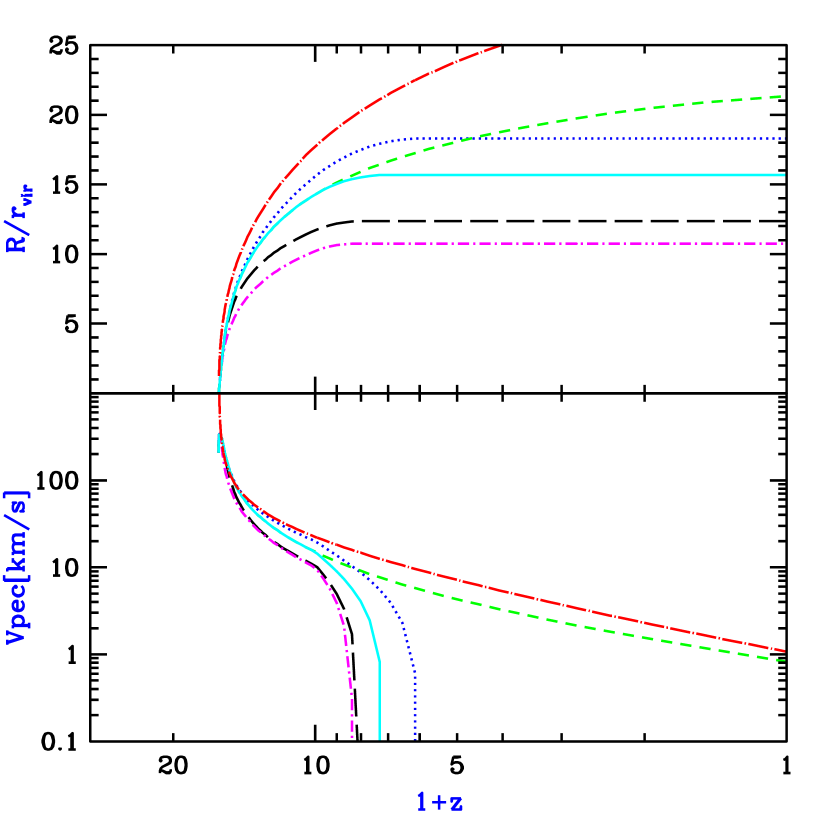
Figure 27: Evolution of a supernova outflow from a $z=15$ halo of circular velocity $V_{c}=20$ km/s. Plotted are the shell comoving radius in units of the virial radius of the source halo (top panel), and the physical peculiar velocity of the shock front (bottom panel). Results are shown for the standard parameters $f_{\rm int}=0.1$, $f_{d}=1$, $f_{\rm wind}=75\%$, and $f_{\rm gas}=50\%$ (solid curve). Also shown for comparison are the cases of no cooling (dotted curve), no reionization (short-dashed curve), $f_{d}=0$ (long-dashed curve), or $f_{\rm wind}=15\%$ and $f_{\rm gas}=10\%$ (dot-short dashed curve), as well as the simple Voit (1996) solution of equation (95) for the standard parameter set (dot-long dashed curve). In cases where the outflow halts, we freeze the radius at the point of maximum expansion.

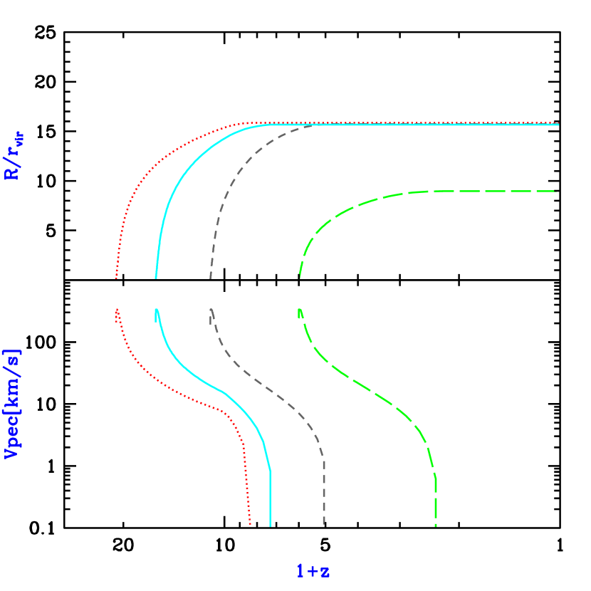
Figure 28: Evolution of supernova outflows at different redshifts. The top and bottom panels are arranged similarly to Figure 27. The $z=15$ outflow (solid curve) is repeated from Figure 27, and it is compared here to outflows with the same parameters but starting at $z=20$ (dotted curve), $z=10$ (short-dashed curve), and $z=5$ (long-dashed curve). A $V_{c}=20$ km/s halo is assumed except for $z=5$, in which case a $V_{c}=42$ km/s halo is assumed to produce the outflow (see text).

Barkana & Loeb (2001, in preparation) derive the overall filling factor of supernova bubbles based on this formalism. In the following subsection we survey previous analytic and numerical work on the collective astrophysical effects of galactic outflows.

7.2 Effect of Outflows on Dwarf Galaxies and on the IGM

Galactic outflows represent a complex feedback process which affects the evolution of cosmic gas through a variety of phenomena. Outflows inject hydrodynamic energy into the interstellar medium of their host galaxy. As shown in the previous subsection, even a small fraction of this energy suffices to eject most of the gas from a dwarf galaxy, perhaps quenching further star formation after the initial burst. At the same time, the enriched gas in outflows can mix with the interstellar medium and with the surrounding IGM, allowing later generations of stars to form more easily because of metal-enhanced cooling. On the other hand, the expanding shock waves may also strip gas in surrounding galaxies and suppress star formation.

Dekel & Silk (1986) attempted to explain the different properties of diffuse dwarf galaxies in terms of the effect of galactic outflows (see also Larson 1974; Vader 1986, 1987). They noted the observed trends whereby lower-mass dwarf galaxies have a lower surface brightness and metallicity, but a higher mass-to-light ratio, than higher mass galaxies. They argued that these trends are most naturally explained by substantial gas removal from an underlying dark matter potential. Galaxies lying in small halos can eject their remaining gas after only a tiny fraction of the gas has turned into stars, while larger galaxies require more substantial star formation before the resulting outflows can expel the rest of the gas. Assuming a wind efficiency $f_{\rm wind}\sim 100\%$, Dekel & Silk showed that outflows in halos below a circular velocity threshold of $V_{\rm crit}\sim 100$ km/s have sufficient energy to expel most of the halo gas. Furthermore, cooling is very efficient for the characteristic gas temperatures associated with $V_{\rm crit}\lesssim 100$ km/s halos, but it becomes less efficient in more massive halos. As a result, this critical velocity is expected to signify a dividing line between bright galaxies and diffuse dwarf galaxies. Although these simple considerations may explain a number of observed trends, many details are still not conclusively determined. For instance, even in galaxies with sufficient energy to expel the gas, it is possible that this energy gets deposited in only a small fraction of the gas, leaving the rest almost unaffected.

Since supernova explosions in an inhomogeneous interstellar medium lead to complicated hydrodynamics, in principle the best way to determine the basic parameters discussed in the previous subsection ($f_{\rm wind}$, $f_{\rm gas}$, and $f_{\rm eject}$) is through detailed numerical simulations of individual galaxies. Mac Low & Ferrara (1999) simulated a gas disk within a $z=0$ dark matter halo. The disk was assumed to be azimuthal and initially smooth. They represented supernovae by a central source of energy and mass, assuming a constant luminosity which is maintained for 50 million years. They found that the hot, metal-enriched ejecta can in general escape from the halo much more easily than the colder gas within the disk, since the hot gas is ejected in a tube perpendicular to the disk without displacing most of the gas in the disk. In particular, most of the metals were expelled except for the case with the most massive halo considered (with $10^{9}M_{\sun}$ in gas) and the lowest luminosity ($10^{37}$ erg/s, or a total injection of $2\times 10^{52}$ erg). On the other hand, only a small fraction of the total gas mass was ejected except for the least massive halo (with $10^{6}M_{\sun}$ in gas), where a luminosity of $10^{38}$ erg/s or more expelled most of the gas. We note that beyond the standard issues of numerical resolution and convergence, there are several difficulties in applying these results to high-redshift dwarf galaxies. Clumping within the expanding shells or the ambient interstellar medium may strongly affect both the cooling and the hydrodynamics. Also, the effect of distributing the star formation throughout the disk is unclear since in that case several characteristics of the problem will change; many small explosions will distribute the same energy over a larger gas volume than a single large explosion [as in the Sedov-Taylor solution (Sedov 1946, 1959; Taylor 1950); see, e.g., equation (95)], and the geometry will be different as each bubble tries to dig its own escape route through the disk. Also, high-redshift disks should be denser by orders of magnitude than $z=0$ disks, due to the higher mean density of the universe at early times. Thus, further numerical simulations of this process are required in order to assess its significance during the reionization epoch.

Some input on these issues also comes from observations. Martin (1999) showed that the hottest extended X-ray emission in galaxies is characterized by a temperature of $\sim 10^{6.7}$ K. This hot gas, which is lifted out of the disk at a rate comparable to the rate at which gas goes into new stars, could escape from galaxies with rotation speeds of $\lesssim 130$ km/s. However, these results are based on a small sample that includes only the most vigorous star-forming local galaxies, and the mass-loss rate depends on assumptions about the poorly understood transfer of mass and energy among the various phases of the interstellar medium.

Many authors have attempted to estimate the overall cosmological effects of outflows by combining simple models of individual outflows with the formation rate of galaxies, obtained via semi-analytic methods (Couchman & Rees 1986; Blanchard, Valls-Gabaud, & Mamon 1992; Tegmark, et al. 1993; Voit 1996; Nath & Trentham 1997; Prunet & Blanchard 2000; Ferrara, Pettini, & Shchekinov 2000; Scannapieco & Broadhurst 2000) or numerical simulations (Gnedin & Ostriker 1997; Gnedin 1998; Cen & Ostriker 1999; Aguirre et al. 2000a). The main goal of these calculations is to explain the characteristic metallicities of different environments as a function of redshift. For example, the IGM is observed to be enriched with metals at redshifts $z\lesssim 5$. Identification of C 4, Si 4 and O 6 absorption lines which correspond to Ly$\alpha$ absorption lines in the spectra of high-redshift quasars has revealed that the low-density IGM has been enriched to a metal abundance (by mass) of $Z_{\rm IGM}\sim 10^{-2.5(\pm 0.5)}Z_{\odot}$, where $Z_{\odot}=0.019$ is the solar metallicity (Meyer & York 1987; Tytler et al. 1995; Songaila & Cowie 1996; Lu et al 1998; Cowie & Songaila 1998; Songaila 1997; Ellison et al. 2000; Prochaska & Wolfe 2000). The metal enrichment has been clearly identified down to H 1 column densities of $\sim 10^{14.5}~{}{\rm cm^{-2}}$. The detailed comparison of cosmological hydrodynamic simulations with quasar absorption spectra has established that the forest of Ly$\alpha$ absorption lines is caused by the smoothly-fluctuating density of the neutral component of the IGM (Cen et al. 1994; Zhang, Anninos & Norman 1995; Hernquist et al. 1996). The simulations show a strong correlation between the H 1 column density and the gas overdensity $\delta_{\rm gas}$ (e.g., Davé et al. 1999), implying that metals were dispersed into regions with an overdensity as low as $\delta_{\rm gas}\sim 3$ or possibly even lower.

In general, dwarf galaxies are expected to dominate metal enrichment at high-redshift for several reasons. As noted above and in the previous subsection, outflows can escape more easily out of the potential wells of dwarfs. Also, at high redshift, massive halos are rare and dwarf halos are much more common. Finally, as already noted, the Sedov-Taylor solution (Sedov 1946, 1959; Taylor 1950) [or equation (95)] implies that for a given total energy and expansion time, multiple small outflows (i.e., caused by explosions with a small individual energy release) fill large volumes more effectively than would a smaller number of large outflows. Note, however, that the strong effect of feedback in dwarf galaxies may also quench star formation rapidly and reduce the efficiency of star formation in dwarfs below that found in more massive galaxies.

Cen & Ostriker (1999) showed via numerical simulation that metals produced by supernovae do not mix uniformly over cosmological volumes. Instead, at each epoch the highest density regions have much higher metallicity than the low-density IGM. They noted that early star formation occurs in the most overdense regions, which therefore reach a high metallicity (of order a tenth of the solar value) by $z\sim 3$, when the IGM metallicity is lower by 1–2 orders of magnitude. At later times, the formation of high-temperature clusters in the highest-density regions suppresses star formation there, while lower-density regions continue to increase their metallicity. Note, however, that the spatial resolution of the hydrodynamic code of Cen & Ostriker is a few hundred kpc, and anything occurring on smaller scales is inserted directly via simple parametrized models. Scannapieco & Broadhurst (2000) implemented expanding outflows within a numerical scheme which, while not a full gravitational simulation, did include spatial correlations among halos. They showed that winds from low-mass galaxies may also strip gas from nearby galaxies (see also Scannapieco, Ferrara, & Broadhurst 2000), thus suppressing star formation in a local neighborhood and substantially reducing the overall abundance of galaxies in halos below a mass of $\sim 10^{10}M_{\sun}$. Although quasars do not produce metals, they may also affect galaxy formation in their vicinity via energetic outflows (Efstathiou & Rees 1988; Babul & White 1991; Silk & Rees 1998; Natarajan, Sigurdsson, & Silk 1998).

Gnedin & Ostriker (1997) and Gnedin (1998) identified another mixing mechanism which, they argued, may be dominant at high redshift ($z\gtrsim 4$). In a collision between two proto-galaxies, the gas components collide in a shock and the resulting pressure force can eject a few percent of the gas out of the merger remnant. This is the merger mechanism, which is based on gravity and hydrodynamics rather than direct stellar feedback. Even if supernovae inject most of their metals in a local region, larger-scale mixing can occur via mergers. Note, however, that Gnedin’s (1998) simulation assumed a comoving star formation rate at $z\gtrsim 5$ of $\sim 1M_{\sun}$ per year per comoving Mpc³, which is 5–10 times larger than the observed rate at redshift 3–4 (§8.1). Aguirre et al. (2000a) used outflows implemented in simulations to conclude that winds of $\sim 300$ km/s at $z\lesssim 6$ can produce the mean metallicity observed at $z\sim 3$ in the Ly$\alpha$ forest. Aguirre et al. (2000b) explored another process, where metals in the form of dust grains are driven to large distances by radiation pressure, thus producing large-scale mixing without displacing or heating large volumes of IGM gas. The success of this mechanism depends on detailed microphysics such as dust grain destruction and the effect of magnetic fields. The scenario, though, may be directly testable because it leads to significant ejection only of elements which solidify as grains.

Feedback from galactic outflows encompasses a large variety of processes and influences. The large range of scales involved, from stars or quasars embedded in the interstellar medium up to the enriched IGM on cosmological scales, make possible a multitude of different, complementary approaches, promising to keep galactic feedback an active field of research.

8 Properties of the Expected Source Population

8.1 The Cosmic Star Formation History

One of the major goals of the study of galaxy formation is to achieve an observational determination and a theoretical understanding of the cosmic star formation history. By now, this history has been sketched out to a redshift $z\sim 4$ (see, e.g., the compilation of Blain et al. 1999a). This is based on a large number of observations in different wavebands. These include various ultraviolet/optical/near-infrared observations (Madau et al. 1996; Gallego et al. 1996; Lilly et al. 1996; Connolly et al. 1997; Treyer et al. 1998; Tresse & Maddox 1998; Pettini et al. 1998a,b; Cowie, Songaila & Barger 1999; Gronwall 1999; Glazebrook et al. 1999; Yan et al. 1999; Flores et al. 1999; Steidel et al. 1999). At the shortest wavelengths, the extinction correction is likely to be large (a factor of $\sim 5$) and is still highly uncertain. At longer wavelengths, the star formation history has been reconstructed from submillimeter observations (Blain et al. 1999b; Hughes et al. 1998) and radio observations (Cram 1998). In the submillimeter regime, a major uncertainty results from the fact that only a minor portion of the total far infrared emission of galaxies comes out in the observed bands, and so in order to estimate the star formation rate it is necessary to assume a spectrum based, e.g., on a model of the dust emission (see the discussion in Chapman et al. 2000). In general, estimates of the star formation rate (hereafter SFR) apply locally-calibrated correlations between emission in particular lines or wavebands and the total SFR. It is often not possible to check these correlations directly on high-redshift populations, and together with the other uncertainties (extinction and incompleteness) this means that current knowledge of the star formation history must be considered to be a qualitative sketch only. Despite the relatively early state of observations, a wealth of new observatories in all wavelength regions promise to greatly advance the field. In particular, NGST  will be able to detect galaxies and hence determine the star formation history out to $z\gtrsim 10$.

Hierarchical models have been used in many papers to match observations on star formation at $z\lesssim 4$ (see, e.g. Baugh et al. 1998; Kauffmann & Charlot 1998; Somerville & Primack 1998, and references therein). In this section we focus on theoretical predictions for the cosmic star formation rate at higher redshifts. The reheating of the IGM during reionization suppressed star formation inside the smallest halos (§6.5). Reionization is therefore predicted to cause a drop in the cosmic SFR. This drop is accompanied by a dramatic fall in the number counts of faint galaxies. Barkana & Loeb (2000b) argued that a detection of this fall in the faint luminosity function could be used to identify the reionization redshift observationally.

A model for the SFR can be constructed based on the extended Press-Schechter theory. The starting point is the abundance of dark matter halos, obtained using the Press-Schechter model. The abundance of halos evolves with redshift as each halo gains mass through mergers with other halos. If $dp[M_{1},t_{1}\rightarrow M,t]$ is the probability that a halo of mass $M_{1}$ at time $t_{1}$ will have merged to form a halo of mass between $M$ and $M+dM$ at time $t>t_{1}$, then in the limit where $t_{1}$ tends to $t$ we obtain an instantaneous merger rate $d^{2}p[M_{1}\rightarrow M,t]/(dM\ dt)$. This quantity was evaluated by Lacey & Cole [1993, their equation (2.18)], and it is the basis for modeling the rate of galaxy formation.

Once a dark matter halo has collapsed and virialized, the two requirements for forming new stars are gas infall and cooling. We assume that by the time of reionization, photo-dissociation of molecular hydrogen (see §3.3) has left only atomic transitions as an avenue for efficient cooling. Before reionization, therefore, galaxies can form in halos down to a circular velocity of $V_{c}\sim 17\ {\rm km\ s}^{-1}$, where this limit is set by cooling. On the other hand, when a volume of the IGM is ionized by stars or quasars, the gas is heated and the increased pressure suppresses gas infall into halos with a circular velocity below $V_{c}\sim 80\ {\rm km\ s}^{-1}$, halting infall below $V_{c}\sim 30\ {\rm km\ s}^{-1}$ (§6.5). Since the suppression acts only in regions that have been heated, the reionization feedback on galaxy formation depends on the fraction of the IGM which is ionized at each redshift. In order to include a gradual reionization in the model, we take the simulations of Gnedin (2000a) as a guide for the redshift interval of reionization.

In general, new star formation in a given galaxy can occur either from primordial gas or from recycled gas which has already undergone a previous burst of star formation. The former occurs when a massive halo accretes gas from the IGM or from a halo which is too small to have formed stars. The latter occurs when two halos, in which a fraction of the gas has already turned to stars, merge and trigger star formation in the remaining gas. Numerical simulations of starbursts in interacting $z=0$ galaxies (e.g., Mihos & Hernquist 1994; 1996) found that a merger triggers significant star formation in a halo even if it merges with a much less massive partner. Preliminary results (Somerville 2000, private communication) from simulations of mergers at $z\sim 3$ find that they remain effective at triggering star formation even when the initial disks are dominated by gas. Regardless of the mechanism, we assume that feedback limits the star formation efficiency, so that only a fraction $\eta$ of the gas is turned into stars.

Given the SFR and the total number of stars in a halo of mass $M$, the luminosity and spectrum can be derived from an assumed stellar initial mass function. We assume an initial mass function which is similar to the one measured locally. If $n(M)$ is the total number of stars with masses less than $M$, then the stellar initial mass function, normalized to a total mass of $1M_{\sun}$, is (Scalo 1998)

$$\frac{dn}{d\ln(M)}=\left\{\begin{array}[]{ll}0.396\,M_{1}^{-0.2}\ ,&0.1<M_{1}<1.0\\ 0.396\,M_{1}^{-1.7}\ ,&1.0<M_{1}<10\\ 0.158\,M_{1}^{-1.3}\ ,&10<M_{1}<100\end{array}\right.$$ (97)

where $M_{1}=M/M_{\sun}$. We assume a metallicity $Z=0.001$, and use the stellar population model results of Leitherer et al. (1999) . We also include a Ly$\alpha$ cutoff in the spectrum due to absorption by the dense Ly$\alpha$ forest. We do not, however, include dust extinction, which could be significant in some individual galaxies despite the low mean metallicity expected at high redshift.

Much of the star formation at high redshift is expected to occur in low mass, faint galaxies, and even NGST  may only detect a fraction of the total SFR. A realistic estimate of this fraction must include the finite resolution of the instrument as well as its detection limit for faint sources (Barkana & Loeb 2000a). We characterize the instrument’s resolution by a minimum circular aperture of angular diameter $\theta_{a}$. We describe the sensitivity of NGST  by $F_{\nu}^{\rm ps}$, the minimum spectral flux, averaged over wavelengths 0.6–3.5$\mu$m, required to detect a point source (i.e., a source which is much smaller than $\theta_{a}$). For an extended source of diameter $\theta_{s}\gg\theta_{a}$, we assume that the signal-to-noise ratio can be improved by using a larger aperture, with diameter $\theta_{s}$. The noise amplitude scales as the square root of the number of noise (sky) photons, or the square root of the corresponding sky area. Thus, the total flux needed for detection of an extended source at a given signal-to-noise threshold is larger than $F_{\nu}^{\rm ps}$ by a factor of $\theta_{s}/\theta_{a}$. We adopt a simple interpolation formula between the regimes of point-like and extended sources, and assume that a source is detectable if its flux is at least $\sqrt{1+(\theta_{s}/\theta_{a})^{2}}\,F_{\nu}^{\rm ps}$.

We combine this result with a model for the distribution of disk sizes at each value of halo mass and redshift (§5.1). We adopt a value of $F_{\nu}^{\rm ps}=0.25$ nJy , assuming a deep 300-hour integration on an 8-meter NGST  and a spectral resolution of 10:1. This resolution should suffice for a $\sim 10\%$ redshift measurement, based on the Ly$\alpha$ cutoff. We also choose the aperture diameter to be $\theta_{a}=0\farcs 06$, close to the expected NGST  resolution at $2\mu$m.

Figure 29 shows our predictions for the star formation history of the universe, adopted from Figure 1 of Barkana & Loeb (2000b) with slight modifications (in the initial mass function and the values of the cosmological parameters). Letting $z_{\rm reion}$ denote the redshift at the end of overlap, we show the SFR for $z_{\rm reion}=6$ (solid curves), $z_{\rm reion}=8$ (dashed curves), and $z_{\rm reion}=10$ (dotted curves). In each pair of curves, the upper one is the total SFR, and the lower one is the fraction detectable with NGST.  The curves assume a star formation efficiency $\eta=10\%$ and an IGM temperature $T_{\rm IGM}=2\times 10^{4}$ K. Although photoionization directly suppresses new gas infall after reionization, it does not immediately affect mergers which continue to trigger star formation in gas which had cooled prior to reionization. Thus, the overall suppression is dominated by the effect on star formation in primordial (unprocessed) gas. The contribution from merger-induced star formation is comparable to that from primordial gas at $z<z_{\rm reion}$, and it is smaller at $z>z_{\rm reion}$. However, the recycled gas contribution to the detectable SFR is dominant at the highest redshifts, since the brightest, highest mass halos form in mergers of halos which themselves already contain stars. Thus, even though most stars at $z>z_{\rm reion}$ form out of primordial, zero-metallicity gas, a majority of stars in detectable galaxies may form out of the small gas fraction that has already been enriched by the first generation of stars.

Points with error bars in Figure 29 are observational estimates of the cosmic SFR per comoving volume at various redshifts (as compiled by Blain et al. 1999a). We choose $\eta=10\%$ to obtain a rough agreement between the models and these observations at $z\sim 3$–4. An efficiency of order this value is also suggested by observations of the metallicity of the Ly$\alpha$ forest at $z=3$ (Haiman & Loeb 1999b). The SFR curves are roughly proportional to the value of $\eta$. Note that in reality $\eta$ may depend on the halo mass, since the effect of supernova feedback may be more pronounced in small galaxies (§7). Figure 29 shows a sharp rise in the total SFR at redshifts higher than $z_{\rm reion}$. Although only a fraction of the total SFR can be detected with NGST,  the detectable SFR displays a definite signature of the reionization redshift. However, current observations at lower redshifts demonstrate the observational difficulty in measuring the SFR directly. The redshift evolution of the faint luminosity function provides a clearer, more direct observational signature. We discuss this topic next.

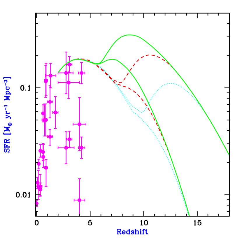
Figure 29: Redshift evolution of the SFR (in $M_{\sun}$ per year per comoving Mpc³), adopted from Figure 1 of Barkana & Loeb (2000b) with slight modifications. Points with error bars are observational estimates (compiled by Blain et al. 1999a). Also shown are model predictions for a reionization redshift $z_{\rm reion}=6$ (solid curves), $z_{\rm reion}=8$ (dashed curves), and $z_{\rm reion}=10$ (dotted curves), with a star formation efficiency $\eta=10\%$. In each pair of curves, the upper one is the total SFR, and the lower one is the fraction detectable with NGST  at a limiting point source flux of 0.25 nJy. We assume the $\Lambda$CDM model (with parameters given at the end of §1).

8.2 Number Counts

8.2.1 Galaxies

As shown in the previous section, the cosmic star formation history should display a signature of the reionization redshift. Much of the increase in the star formation rate beyond the reionization redshift is due to star formation occurring in very small, and thus faint, galaxies. This evolution in the faint luminosity function constitutes the clearest observational signature of the suppression of star formation after reionization.

Figure 30 shows the predicted redshift distribution in $\Lambda$CDM (with parameters given at the end of §1) of galaxies observed with NGST.  The plotted quantity is $dN/dz$, where $N$ is the number of galaxies per NGST  field of view ($4\arcmin\times 4\arcmin$). The model predictions are shown for a reionization redshift $z_{\rm reion}=6$ (solid curve), $z_{\rm reion}=8$ (dashed curve), and $z_{\rm reion}=10$ (dotted curve), with a star formation efficiency $\eta=10\%$. All curves assume a point-source detection limit of 0.25 nJy. This plot is updated from Figure 7 of Barkana & Loeb (2000a) in that redshifts above $z_{\rm reion}$ are included.

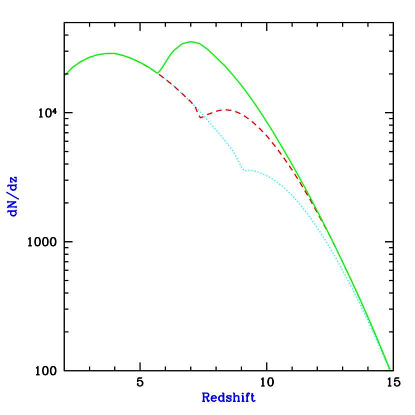
Figure 30: Predicted redshift distribution of galaxies observed with NGST,  adopted and modified from Figure 7 of Barkana & Loeb (2000a). The distribution in the $\Lambda$CDM model (with parameters given at the end of §1), with a star formation efficiency $\eta=10\%$, is shown for a reionization redshift $z_{\rm reion}=6$ (solid curve), $z_{\rm reion}=8$ (dashed curve), and $z_{\rm reion}=10$ (dotted curve). The plotted quantity is $dN/dz$, where $N$ is the number of galaxies per NGST  field of view. All curves assume a limiting point source flux of 0.25 nJy.

Clearly, thousands of galaxies are expected to be found at high redshift. This will allow a determination of the luminosity function at many redshift intervals, and thus a measurement of its evolution. As the redshift is increased, the luminosity function is predicted to gradually change shape during the overlap era of reionization. Figure 31 shows the predicted evolution of the luminosity function for various values of $z_{\rm reion}$. This Figure is adopted from Figure 2 of Barkana & Loeb (2000b) with modifications (in the initial mass function, the values of the cosmological parameters, and the plot layout). All curves show $d^{2}N/(dz\ d\ln F_{\nu}^{\rm ps})$, where $N$ is the total number of galaxies in a single field of view of NGST,  and $F_{\nu}^{\rm ps}$ is the limiting point source flux at 0.6–3.5$\mu$m for NGST.  Each panel shows the result for a reionization redshift $z_{\rm reion}=6$ (solid curve), $z_{\rm reion}=8$ (dashed curve), and $z_{\rm reion}=10$ (dotted curve). Figure 31 shows the luminosity function as observed at $z=5$ (upper left panel) and (proceeding clockwise) at $z=7$, $z=9$, and $z=11$. Although our model assigns a fixed luminosity to all halos of a given mass and redshift, in reality such halos would have some dispersion in their merger histories and thus in their luminosities. We thus include smoothing in the plotted luminosity functions. Note the enormous increase in the number density of faint galaxies in a pre-reionization universe. Observing this dramatic increase toward high redshift would constitute a clear detection of reionization and of its major effect on galaxy formation.

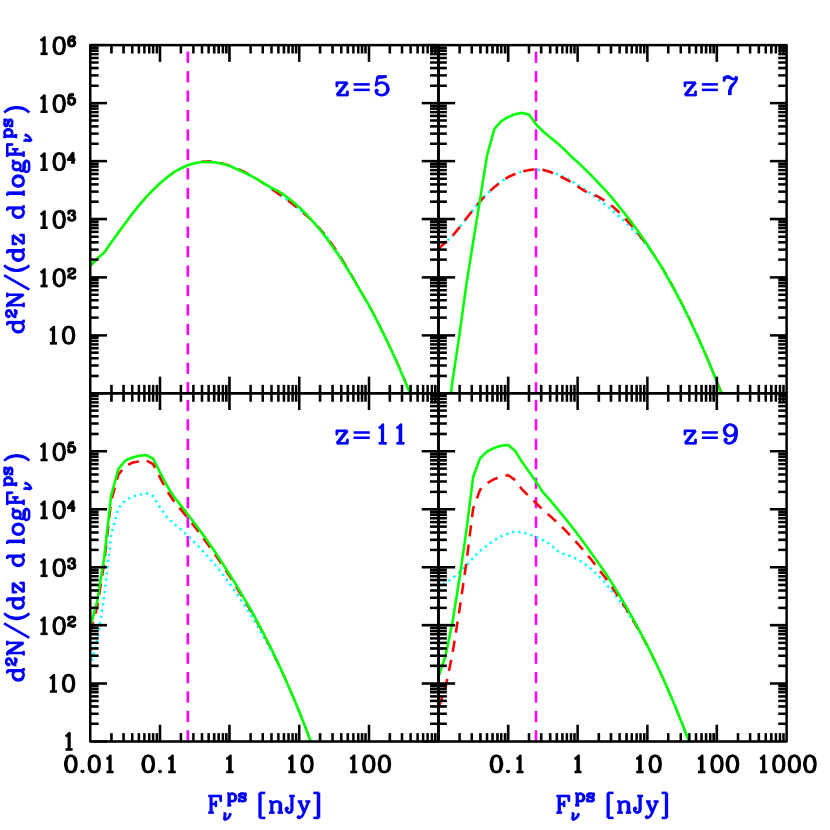
Figure 31: Predicted luminosity function of galaxies at a fixed redshift, adopted and modified from Figure 2 of Barkana & Loeb (2000b). With $\eta=10\%$, the curves show $d^{2}N/(dz\ d\ln F_{\nu}^{\rm ps})$, where $N$ is the total number of galaxies in a single field of view of NGST,  and $F_{\nu}^{\rm ps}$ is the limiting point source flux averaged over 0.6–3.5$\mu$m for NGST.  The luminosity function is shown at $z=5$, $z=7$, $z=9$, and $z=11$, with redshift increasing clockwise starting with the upper left panel. Each case assumes the $\Lambda$CDM model (with parameters given at the end of §1) and a reionization redshift $z_{\rm reion}=6$ (solid curves), $z_{\rm reion}=8$ (dashed curves), or $z_{\rm reion}=10$ (dotted curves). The expected NGST  detection limit is shown by the vertical dashed line.

8.2.2 Quasars

Dynamical studies indicate that massive black holes exist in the centers of most nearby galaxies (Richstone et al. 1998; Kormendy & Ho 2000; Kormendy 2000, and references therein). This leads to the profound conclusion that black hole formation is a generic consequence of galaxy formation. The suggestion that massive black holes reside in galaxies and power quasars dates back to the sixties (Zel’dovich 1964; Salpeter 1964; Lynden-Bell 1969). Efstathiou & Rees (1988) pioneered the modeling of quasars in the modern context of galaxy formation theories. The model was extended by Haehnelt & Rees (1993) who added more details concerning the black hole formation efficiency and lightcurve. Haiman & Loeb (1998) and Haehnelt, Natarajan, & Rees (1998) extrapolated the model to high redshifts. All of these discussions used the Press-Schechter theory to describe the abundance of galaxy halos as a function of mass and redshift. More recently, Kauffmann & Haehnelt (2000; also Haehnelt & Kauffmann 2000) embedded the description of quasars within semi-analytic modeling of galaxy formation, which uses the extended Press-Schechter formalism to describe the merger history of galaxy halos.

In general, the predicted evolution of the luminosity function of quasars is constrained by the need to match the observed quasar luminosity function at redshifts $z\lesssim 5$, as well as data from the Hubble Deep Field (HDF) on faint point-sources. Prior to reionization, we may assume that quasars form only in galaxy halos with a circular velocity $\gtrsim 10~{}{\rm km~{}s^{-1}}$ (or equivalently a virial temperature $\gtrsim 10^{4}$ K), for which cooling by atomic transitions is effective. After reionization, quasars form only in galaxies with a circular velocity $\gtrsim 50\ {\rm km~{}s^{-1}}$, for which substantial gas accretion from the warm ($\sim 10^{4}$ K) IGM is possible. The limits set by the null detection of quasars in the HDF are consistent with the number counts of quasars which are implied by these thresholds (Haiman, Madau, & Loeb 1999).

For spherical accretion of ionized gas, the bolometric luminosity emitted by a black hole has a maximum value beyond which radiation pressure prevents gas accretion. This Eddington luminosity (Eddington 1926) is derived by equating the radiative repulsive force on a free electron to the gravitational attractive force on an ion in the plasma,

$${L\sigma_{T}\over 4\pi r^{2}c}={GM_{\rm bh}\mu_{e}m_{p}\over r^{2}}\ ,$$ (98)

where $\sigma_{T}=6.65\times 10^{-25}~{}{\rm cm^{2}}$ is the Thomson cross-section, $\mu_{e}m_{p}$ is the average ion mass per electron, and $M_{\rm bh}$ is the black hole mass. Since both forces scale as $r^{-2}$, the limiting Eddington luminosity is independent of radius $r$ in the Newtonian regime, and for gas of primordial composition is given by,

$$L_{E}={4\pi cGM_{\rm bh}\mu_{e}m_{p}\over\sigma_{T}}=1.45\times 10^{46}\left({M_{\rm bh}\over 10^{8}M_{\odot}}\right)~{}{\rm erg~{}s^{-1}}\ .$$ (99)

Generically, the Eddington limit applies to within a factor of order unity also to simple accretion flows in a non-spherical geometry (Frank, King, & Raine 1992).

The total luminosity of a black hole is related to its mass accretion rate by the radiative efficiency, $\epsilon$,

$$L=\epsilon\dot{M}_{\rm bh}c^{2}.$$ (100)

For accretion through a thin Keplerian disk onto a Schwarzschild (non-rotating) black hole, $\epsilon=5.7\%$, while for a maximally rotating Kerr black hole, $\epsilon=42\%$ (Shapiro & Teukolsky 1983, p. 429). The thin disk configuration, for which these high radiative efficiencies are attainable, exists for $L_{\rm disk}\lesssim 0.5L_{E}$ (Laor & Netzer 1989) .

The accretion time can be defined as

$$\tau={M_{\rm bh}\over{\dot{M}}_{\rm bh}}=4\times 10^{7}~{}{\rm yr}\left(\epsilon\over 0.1\right)\left({L\over L_{E}}\right)^{-1}\ .$$ (101)

This time is comparable to the dynamical time inside the central kpc of a typical galaxy, $t_{\rm dyn}\sim({\rm 1~{}kpc}/100~{}{\rm km~{}s^{-1}})=10^{7}~{}{\rm yr}$. As long as its fuel supply is not limited and $\epsilon$ is constant, a black hole radiating at the Eddington limit will grow its mass exponentially with an $e$-folding time equal to $\tau$. The fact that $\tau$ is much shorter than the age of the universe even at high redshift implies that black hole growth is mainly limited by the feeding rate ${\dot{M}}_{\rm bh}(t)$, or by the total fuel reservoir, and not by the Eddington limit.

The “simplest model” for quasars involves the following three assumptions (Haiman & Loeb 1998):

(i) A fixed fraction of the baryons in each “newly formed” galaxy ends up making a central black hole.

(ii) Each black hole shines at its maximum (Eddington) luminosity for a universal amount of time.

(iii) All black holes share the same emission spectrum during their luminous phase.

Note that these assumptions relate only to the most luminous phase of the black hole accretion process, and they may not be valid during periods when the radiative efficiency or the mass accretion rate is very low. Such periods are not of interest here since they do not affect the luminosity function of bright quasars, which is the observable we wish to predict. The first of the above assumptions is reasonable as long as the fraction of virialized baryons in the universe is much smaller than unity; it does not include a separate mechanism for fueling black hole growth during mergers of previously-formed galaxies, and thus, under this assumption, black holes would not grow in mass once most of the baryons were virialized. The second hypothesis is motivated by the fact that for a sufficiently high fueling rate (which may occur in the early stage of the collapse/merger of a galaxy), quasars are likely to shine at their maximum possible luminosity. The resulting luminosity should be close to the Eddington limit over a period of order $\tau$. The third assumption can be implemented by incorporating the average quasar spectrum measured by Elvis et al. (1994).

At high redshifts the number of “newly formed” galaxies can be estimated based on the time-derivative of the Press-Schechter mass function, since the collapsed fraction of baryons is small and most galaxies form out of the unvirialized IGM. Haiman & Loeb (1998, 1999a) have shown that the above simple prescription provides an excellent fit to the observed evolution of the luminosity function of bright quasars between redshifts $2.6<z<4.5$ (see the analytic description of the existing data in Pei 1995). The observed decline in the abundance of bright quasars (Schneider, Schmidt, & Gunn 1991; Pei 1995) results from the deficiency of massive galaxies at high redshifts. Consequently, the average luminosity of quasars declines with increasing redshift. The required ratio between the mass of the black hole and the total baryonic mass inside a halo is $M_{\rm bh}/M_{\rm gas}=10^{-3.2}{\Omega_{m}}/\Omega_{b}=5.5\times 10^{-3}$, comparable to the typical value of $\sim 2$–$6\times 10^{-3}$ found for the ratio of black hole mass to spheroid mass in nearby elliptical galaxies (Magorrian et al. 1998; Kormendy 2000). The required lifetime of the bright phase of quasars is $\sim 10^{6}$ yr. Figure 32 shows the most recent prediction of this model (Haiman & Loeb 1999a) for the number counts of high-redshift quasars, taking into account the above-mentioned thresholds for the circular velocities of galaxies before and after reionization.

We do, however, expect a substantial intrinsic scatter in the ratio $M_{\rm bh}/M_{\rm gas}$. Observationally, the scatter around the average value of $\log_{10}(M_{\rm bh}/L)$ is 0.3 (Magorrian et al. 1998), while the standard deviation in $\log_{10}(M_{\rm bh}/M_{\rm gas})$ has been found to be $\sigma\sim 0.5$. Such an intrinsic scatter would flatten the predicted quasar luminosity function at the bright end, where the luminosity function is steeply declining. However, Haiman & Loeb (1999a) have shown that the flattening introduced by the scatter can be compensated for through a modest reduction in the fitted value for the average ratio between the black hole mass and halo mass by $\sim 50\%$ in the relevant mass range ($10^{8}~{}{\rm M_{\odot}}\lesssim M_{\rm bh}\lesssim 10^{10}~{}{\rm M_{\odot}}$).

In reality, the relation between the black hole and halo masses may be more complicated than linear. Models with additional free parameters, such as a non-linear (mass and redshift dependent) relation between the black hole and halo mass, can also produce acceptable fits to the observed quasar luminosity function (Haehnelt et al. 1998). The nonlinearity in a relation of the type $M_{\rm bh}\propto M_{\rm halo}^{\alpha}$ with $\alpha>1$, may be related to the physics of the formation process of low-luminosity quasars(Haehnelt et al. 1998; Silk & Rees 1998), and can be tuned so as to reproduce the black hole reservoir with its scatter in the local universe (Cattaneo, Haehnelt, & Rees 1999). Recently, a tight correlation between the masses of black holes and the velocity dispersions of the bulges in which they reside, $\sigma$, was identified in nearby galaxies. Ferrarese & Merritt (2000; see also Merritt & Ferrarese 2001) inferred a correlation of the type $M_{\rm bh}\propto\sigma^{4.72\pm 0.36}$, based on a selected sample of a dozen galaxies with reliable $M_{\rm bh}$ estimates, while Gebhardt et al. (2000a,b) have found a somewhat shallower slope, $M_{\rm bh}\propto\sigma^{3.75(\pm 0.3)}$ based on a significantly larger sample. A non-linear relation of $M_{\rm bh}\propto\sigma^{5}\propto M_{\rm halo}^{5/3}$ has been predicted by Silk & Rees (1998) based on feedback considerations, but the observed relation also follows naturally in the standard semi-analytic models of galaxy formation (Haehnelt & Kauffmann 2000).

Figure 32 shows the predicted number counts in the “simplest model” described above (Haiman & Loeb 1999a), normalized to a $5^{\prime}\times 5^{\prime}$ field of view. Figure 32 shows separately the number per logarithmic flux interval of all objects with redshifts $z>5$ (thin lines), and $z>10$ (thick lines). The number of detectable sources is high; NGST  will be able to probe of order $100$ quasars at $z>10$, and $\sim 200$ quasars at $z>5$ per $5^{\prime}\times 5^{\prime}$ field of view. The bright-end tail of the number counts approximately follows a power law, with $dN/dF_{\nu}\propto F_{\nu}^{-2.5}$. The dashed lines show the corresponding number counts of “star-clusters”, assuming that each halo shines due to a starburst that converts a fraction of 2% (long-dashed) or 20% (short-dashed) of the gas into stars.

Similar predictions can be made in the X-ray regime. Figure 33 shows the number counts of high-redshift X-ray quasars in the above “simplest model”. This model fits the X-ray luminosity function of quasars at $z\sim 3.5$ as observed by ROSAT (Miyaji, Hasinger, & Schmidt 2000), using the same parameters necessary to fit the optical data (Pei 1995). Deep optical or infrared follow-ups on deep images taken with the Chandra X-ray satellite (CXO; see, e.g., Mushotzky et al. 2000; Barger et al. 2001; Giacconi et al. 2000) may be used to test these predictions in the relatively near future.

Figure 32: Infrared number counts of quasars (averaged over the wavelength interval of $1$–$3.5\mu$m) based on the “simplest quasar model” of Haiman & Loeb (1999b). The solid curves refer to quasars, while the long/short dashed curves correspond to star clusters with low/high normalization for the star formation efficiency. The curves labeled “5” or “10” show the cumulative number of objects with redshifts above $z=5$ or 10.

Figure 33: Total number of quasars with redshift exceeding $z=5$, $z=7$, and $z=10$ as a function of observed X-ray flux in the CXO detection band (from Haiman & Loeb 1999a). The numbers are normalized per $17^{\prime}\times 17^{\prime}$ area of the sky. The solid curves correspond to a cutoff in circular velocity for the host halos of $v_{\rm circ}\geq 50~{}{\rm km~{}s^{-1}}$, the dashed curves to a cutoff of $v_{\rm circ}\geq 100~{}{\rm km~{}s^{-1}}$. The vertical dashed line shows the CXO sensitivity for a 5$\sigma$ detection of a point source in an integration time of $5\times 10^{5}$ seconds.

The “simplest model” mentioned above predicts that black holes and stars make comparable contributions to the ionizing background prior to reionization. Consequently, the reionization of hydrogen and helium is predicted to occur roughly at the same epoch. A definitive identification of the He 2 reionization redshift will provide another powerful test of this model. Further constraints on the lifetime of the active phase of quasars may be provided by future measurements of the clustering properties of quasars (Haehnelt et al. 1998; Martini & Weinberg 2001; Haiman & Hui 2000).

8.2.3 Supernovae

The detection of galaxies and quasars becomes increasingly difficult at a higher redshift. This results both from the increase in the luminosity distance and the decrease in the average galaxy mass with increasing redshift. It therefore becomes advantageous to search for transient sources, such as supernovae or $\gamma$-ray bursts, as signposts of high-redshift galaxies (Miralda-Escudé & Rees 1997). Prior to or during the epoch of reionization, such sources are likely to outshine their host galaxies.

The metals detected in the IGM (see §7.2) signal the existence of supernova (SN) explosions at redshifts $z\gtrsim 5$. Since each SN produces an average of $\sim 1M_{\odot}$ of heavy elements (Woosley & Weaver 1995), the inferred metallicity of the IGM, $Z_{\rm IGM}$, implies that there should be a supernova at $z\gtrsim 5$ for each $\sim 1.7\times 10^{4}M_{\odot}\times(Z_{\rm IGM}/10^{-2.5}Z_{\odot})^{-1}$ of baryons in the universe. We can therefore estimate the total supernova rate, on the entire sky, necessary to produce these metals at $z\sim 5$. Consider all SNe which are observed over a time interval $\Delta t$ on the whole sky. Due to the cosmic time dilation, they correspond to a narrow redshift shell centered at the observer of proper width $c\Delta t/(1+z)$. In a flat ${\Omega_{m}}=0.3$ cosmology, the total mass of baryons in a narrow redshift shell of width $c\Delta t/(1+z)$ around $z=5$ is $\sim[4\pi(1+z)^{-3}(1.8c/H_{0})^{2}c\Delta t]\times[\Omega_{b}(3H_{0}^{2}/8\pi G)(1+z)^{3}]=4.9\,c^{3}\Omega_{b}\Delta t/G$. Hence, for $h=0.7$ the total supernova rate across the entire sky at $z\gtrsim 5$ is estimated to be (Miralda-Escudé & Rees 1997),

$${\dot{N}}_{SN}\approx 10^{8}\left({Z_{\rm IGM}\over 10^{-2.5}Z_{\odot}}\right)\ {\rm yr}^{-1}\ ,$$ (102)

or roughly one SN per square arcminute per year.

The actual SN rate at a given observed flux threshold is determined by the star formation rate per unit comoving volume as a function of redshift and the initial mass function of stars (Madau, della Valle, & Panagia 1998; Woods & Loeb 1998; Sullivan et al. 2000). To derive the relevant expression for flux-limited observations, we consider a general population of transient sources which are standard candles in peak flux and are characterized by a comoving rate per unit volume $R(z)$. The observed number of new events per unit time brighter than flux $F_{\nu}$ at observed wavelength $\lambda$ for such a population is given by

$$\dot{N}(F_{\nu};\lambda)=\int_{0}^{z_{{\rm max}(F_{\nu};\lambda)}}R(z)(1+z)^{-1}(dV_{\rm c}/dz)dz,$$ (103)

where $z_{\rm max}(F_{\nu},\lambda)$ is the maximum redshift at which a source will appear brighter than $F_{\nu}$ at an observed wavelength $\lambda=c/\nu$, and $dV_{\rm c}$ is the cosmology-dependent comoving volume element corresponding to a redshift interval $dz$. The above integrand includes the $(1+z)$ reduction in the apparent rate due to the cosmic time dilation.

Figure 34 shows the predicted SN rate as a function of limiting flux in various bands (Woods & Loeb 1998), based on the comoving star formation rate as a function of redshift that was determined empirically by Madau (1997). The actual star formation rate may be somewhat higher due to corrections for dust extinction (for a recent compilation of current data, see Blain & Natarajan 2000). The dashed lines correspond to Type Ia SNe and the dotted lines to Type II SNe. For comparison, the solid lines indicate two crude estimates for the rate of $\gamma$-ray burst afterglows, which are discussed in detail in the next section.

Figure 34: Predicted cumulative rate $\dot{N}(>F_{\nu})$ per year per square degree of supernovae at four wavelengths, corresponding to the $K$, $R$, $B$, and $U$ bands (from Woods & Loeb 1998). The broken lines refer to different supernova types, namely SNe Ia (dashed curves) and SNe II (dotted curves). For comparison, the solid curves show estimates for the rates of gamma-ray burst (GRB) afterglows; the lower solid curve assumes the best-fit rate and luminosity for GRB sources which trace the star formation history (Wijers et al. 1998), while the upper solid curve assumes the best-fit values for a non-evolving GRB population.

Equation (103) is appropriate for a threshold experiment, one which monitors the sky continuously and triggers when the detected flux exceeds a certain value, and hence identifies the most distant sources only when they are near their peak flux. For search strategies which involve taking a series of “snapshots” of a field and looking for variations in the flux of sources in successive images, one does not necessarily detect most sources near their peak flux. In this case, the total  number of events (i.e., not  per unit time) brighter than $F_{\nu}$ at observed wavelength $\lambda$ is given by

$$N(F_{\nu};\lambda)=\int_{0}^{\infty}R(z)t_{\star}(z;F_{\nu},\lambda)(dV_{\rm c}/dz)dz,$$ (104)

where $t_{\star}(z;F_{\nu},\lambda)$ is the rest-frame duration over which an event will be brighter than the limiting flux $F_{\nu}$ at redshift $z$. This is a naive estimate of the so-called “control time”; in practice, the effective duration over which an event can be observed is shorter, owing to the image subtraction technique, host galaxy magnitudes, and a number of other effects which reduce the detection efficiency (Pain et al. 1996). Figure 35 shows the predicted number counts of SNe as a function of limiting flux for the parameters used in Figure 34 (Woods & Loeb 1998).

Figure 35: Cumulative number counts $N(>F_{\nu})$ per square degree (from Woods & Loeb 1998). The notation is the same as in Figure 34.

Supernovae also produce dust which could process the emission spectrum of galaxies. Although produced in galaxies, the dust may be expelled together with the metals out of galaxies by supernova-driven winds. Loeb & Haiman (1997) have shown that if each supernova produces $\sim 0.3\,M_{\odot}$ of galactic dust, and some of the dust is expelled together with metals out of the shallow potential wells of the early dwarf galaxies, then the optical depth for extinction by intergalactic dust may reach a few tenths at $z\sim 10$ for observed wavelengths of $\sim 0.5$–$1\,\mu$m [see Todini & Ferrara (2000) for a detailed discussion on the production of dust in primordial Type II SNe]. The opacity in fact peaks in this wavelength band since at $z\sim 10$ it corresponds to rest-frame UV, where normal dust extinction is most effective. In these estimates, the amplitude of the opacity is calibrated based on the observed metallicity of the IGM at $z\lesssim 5$. The intergalactic dust absorbs the UV background at the reionization epoch and re-radiates it at longer wavelengths. The flux and spectrum of the infrared background which is produced at each redshift depends sensitively on the distribution of dust around the ionizing sources, since the deviation of the dust temperature from the microwave background temperature depends on the local flux of UV radiation that it is exposed to. For reasonable choices of parameters, dust could lead to a significant spectral distortion of the microwave background spectrum that could be measured by a future spectral mission, going beyond the upper limit derived by the COBE satellite (Fixsen et al. 1996).

The metals produced by supernovae may also yield strong molecular line emission. Silk & Spaans (1997) pointed out that the rotational line emission of CO by starburst galaxies is enhanced at high redshift due to the increasing temperature of the cosmic microwave background, which affects the thermal balance and the level populations of the atomic and molecular species. They found that the future Millimeter Array (MMA) could detect a starburst galaxy with a star formation rate of $\sim 30\,{\rm M_{\odot}~{}yr^{-1}}$ equally well at $z=5$ and $z=30$ because of the increasing cosmic microwave background temperature with redshift. Line emission may therefore be a more powerful probe of the first bright galaxies than continuum emission by dust.

8.2.4 Gamma Ray Bursts

The past decade has seen major observational breakthroughs in the study of Gamma Ray Burst (GRB) sources. The Burst and Transient Source Experiment (BATSE) on board the Compton Gamma Ray Observatory (Meegan et al. 1992) showed that the GRB population is distributed isotropically across the sky, and that there is a deficiency of faint GRBs relative to a Euclidean distribution. These were the first observational clues indicating a cosmological distance scale for GRBs. The localization of GRBs by X-ray observations with the BeppoSAX satellite (Costa et al. 1997) allowed the detection of afterglow emission at optical (e.g., van Paradijs et al. 1997, 2000) and radio (e.g., Frail et al. 1997) wavelengths up to more than a year following the events (Fruchter et al. 1999; Frail et al. 2000). The afterglow emission is characterized by a broken power-law spectrum with a peak frequency that declines with time. The radiation is well-fitted by a model consisting of synchrotron emission from a decelerating blast wave (Blandford & McKee 1976), created by the GRB explosion in an ambient medium, with a density comparable to that of the interstellar medium of galaxies (Waxman 1997; Sari, Piran, & Narayan 1998; Wijers & Galama 1999; Mészáros 1999; but see also Chevalier & Li 2000). The detection of spectral features, such as metal absorption lines in some optical afterglows (Metzger et al. 1997) and emission lines from host galaxies (Kulkarni et al. 2000), allowed an unambiguous identification of cosmological distances to these sources.

The nature of the central engine of GRBs is still unknown. Since the inferred energy release, in cases where it can be securely calibrated (Freedman & Waxman 2001; Frail et al. 2000), is comparable to that in a supernova, $\sim 10^{51}~{}{\rm erg}$, most popular models relate GRBs to stellar remnants such as neutron stars or black holes (Eichler et al. 1989; Narayan, Paczyński, & Piran 1992; Paczyński 1991; Usov 1992; Mochkovitch et al. 1993; Paczyński 1998; MacFadyen & Woosley 1999). Recently it has been claimed that the late evolution of some rapidly declining optical afterglows shows a component which is possibly associated with supernova emission (e.g., Bloom et al. 1999; Reichart 1999). If the supernova association is confirmed by detailed spectra of future afterglows, the GRB phenomenon will be linked to the terminal evolution of massive stars.

Any association of GRBs with the formation of single compact stars implies that the GRB rate should trace the star formation history of the universe (Totani 1997; Sahu et al. 1997; Wijers et al. 1998; but see Krumholz, Thorsett & Harrison 1998). Owing to their high brightness, GRB afterglows could in principle be detected out to exceedingly high redshifts. Just as for quasars, the broad-band emission of GRB afterglows can be used to probe the absorption properties of the IGM out to the reionization epoch at redshift $z\sim 10$. Lamb & Reichart (2000) extrapolated the observed gamma-ray and afterglow spectra of known GRBs to high redshifts and emphasized the important role that their detection could play in probing the IGM (see also Miralda-Escudé 1998). In particular, the broad-band afterglow emission can be used to probe the ionization and metal-enrichment histories of the intervening IGM during the epoch of reionization.

Ciardi & Loeb (2000) showed that unlike other sources (such as galaxies and quasars), which fade rapidly with increasing redshift, the observed infrared flux from a GRB afterglow at a fixed observed age is only a weak function of its redshift (Figure 36). A simple scaling of the long-wavelength spectra and the temporal evolution of afterglows with redshift implies that at a fixed time-lag after the GRB in the observer’s frame, there is only a mild change in the observed flux at infrared or radio wavelengths with increasing redshift. This results in part from the fact that afterglows are brighter at earlier times, and that a given observed time refers to an earlier intrinsic time in the source frame as the source redshift increases. The “apparent brightening” of GRB afterglows with redshift could be further enhanced by the expected increase with redshift of the mean density of the interstellar medium of galaxies (Wood & Loeb 2000). Figure 37 shows the expected number counts of GRB afterglows, assuming that the GRB rate is proportional to the star formation rate and that the characteristic energy output of GRBs is $\sim 10^{52}~{}{\rm erg}$ and is isotropic. The figure implies that at any time there should be of order $\sim 15$ GRBs with redshifts $z\gtrsim 5$ across the sky which are brighter than $\sim 100$ nJy at an observed wavelength of $\sim 2\mu$m. The infrared spectrum of these sources could be measured with NGST  as a follow-up on their early X-ray localization with $\gamma$-ray or X-ray detectors. Prior to reionization, the spectrum of GRB afterglows could reveal the long sought-after Gunn-Peterson trough (Gunn & Peterson 1965) due to absorption by the neutral IGM.

The predicted GRB rate and flux are subject to uncertainties regarding the beaming of the emission. The beaming angle may vary with observed time due to the decline with time of the Lorentz factor $\gamma(t)$ of the emitting material. As long as the Lorentz factor is significantly larger than the inverse of the beaming angle (i.e., $\gamma\gtrsim\theta^{-1}$), the afterglow flux behaves as if it were emitted by a spherically-symmetric fireball with the same explosion energy per unit solid angle. However, the lightcurve changes as soon as $\gamma$ declines below $\theta^{-1}$, due to the lateral expansion of the jet (Rhoads 1997, 1999a,b; Panaitescu & Mészáros 1999). Finally, the isotropization of the energy ends when the expansion becomes sub-relativistic, at which point the remnant recovers the spherically-symmetric Sedov-Taylor solution (Sedov 1946, 1959; Taylor 1950) with the total remaining energy. When $\gamma\sim 1$, the emission occurs from a roughly spherical fireball with the effective explosion energy per solid angle reduced by a factor of $(2\pi\theta^{2}/4\pi)$ relative to that at early times, representing the fraction of sky around the GRB source which is illuminated by the initial two (opposing) jets of angular radius $\theta$ (see Ciardi & Loeb 2000 for the impact of this effect on the number counts). The calibration of the GRB event rate per comoving volume, based on the number counts of GRBs (Wijers et al. 1998), is inversely proportional to this factor.

The main difficulty in using GRBs as probes of the high-redshift universe is that they are rare, and hence their detection requires surveys which cover a wide area of the sky. The simplest strategy for identifying high-redshift afterglows is through all-sky surveys in the $\gamma$-ray or X-ray regimes. In particular, detection of high-redshift sources will become feasible with the high trigger rate provided by the forthcoming Swift  satellite, to be launched in 2003 (see http://swift.gsfc.nasa.gov/, for more details). Swift  is expected to localize $\sim$300 GRBs per year, and to re-point within 20–70 seconds its on-board X-ray and UV-optical instrumentation for continued afterglow studies. The high-resolution GRB coordinates obtained by Swift  will be transmitted to Earth within $\sim$50 seconds. Deep follow-up observations will then be feasible from the ground or using the highly-sensitive infrared instruments on board NGST.  Swift  will be sufficiently sensitive to trigger on the $\gamma$-ray emission from GRBs at redshifts $z\gtrsim 10$ (Lamb & Reichart 2000).

8.3 Distribution of Disk Sizes

Given the distribution of disk sizes at each value of halo mass and redshift (§5.1) and the number counts of galaxies (§8.2.1), we derive the predicted size distribution of galactic disks. Note that although frequent mergers at high redshift may disrupt these disks and alter the morphologies of galaxies, the characteristic sizes of galaxies will likely not change dramatically. We show in Figure 38 [an updated version of Figure 6 of Barkana & Loeb (2000a)] the distribution of galactic disk sizes at various redshifts, in the $\Lambda$CDM model (with parameters given at the end of §1). Given $\theta$ in arcseconds, each curve shows the fraction of the total number counts contributed by sources larger than $\theta$. The diameter $\theta$ is measured out to one exponential scale length. We show three pairs of curves, at $z=2$, $z=5$ and $z=10$ (from right to left). Each pair includes the distribution for all galaxies (dashed line), and for galaxies detectable by NGST  (solid line) with a limiting point source flux of 0.25 nJy and with an efficiency $\eta=10\%$ assumed for the galaxies. The vertical dotted line indicates the expected NGST  resolution of $0\farcs 06$.

Figure 36: Observed flux from a $\gamma$-ray burst afterglow as a function of redshift (from Ciardi & Loeb 2000). The two sets of curves refer to a photon frequency $\nu=6\times 10^{14}$ Hz ($\lambda_{obs}=5000$ Å, thin lines) and $\nu=1.5\times 10^{14}$ Hz ($\lambda_{obs}=2\mu$m, thick lines). Each set shows different observed times after the GRB trigger; from top to bottom: 1 hour (solid line), 1 day (dotted) and 10 days (dashed). The sharp suppression for 5000 Å  at $z\gtrsim 4.5$ is due to IGM absorption.

Figure 37: Predicted number of GRB afterglows per square degree with observed flux greater than $F$, at several different observed wavelengths (from Ciardi & Loeb 2000). From right to left, the observed wavelength equals 10 cm, 1 mm, 2 $\mu$m and 5000 Å.

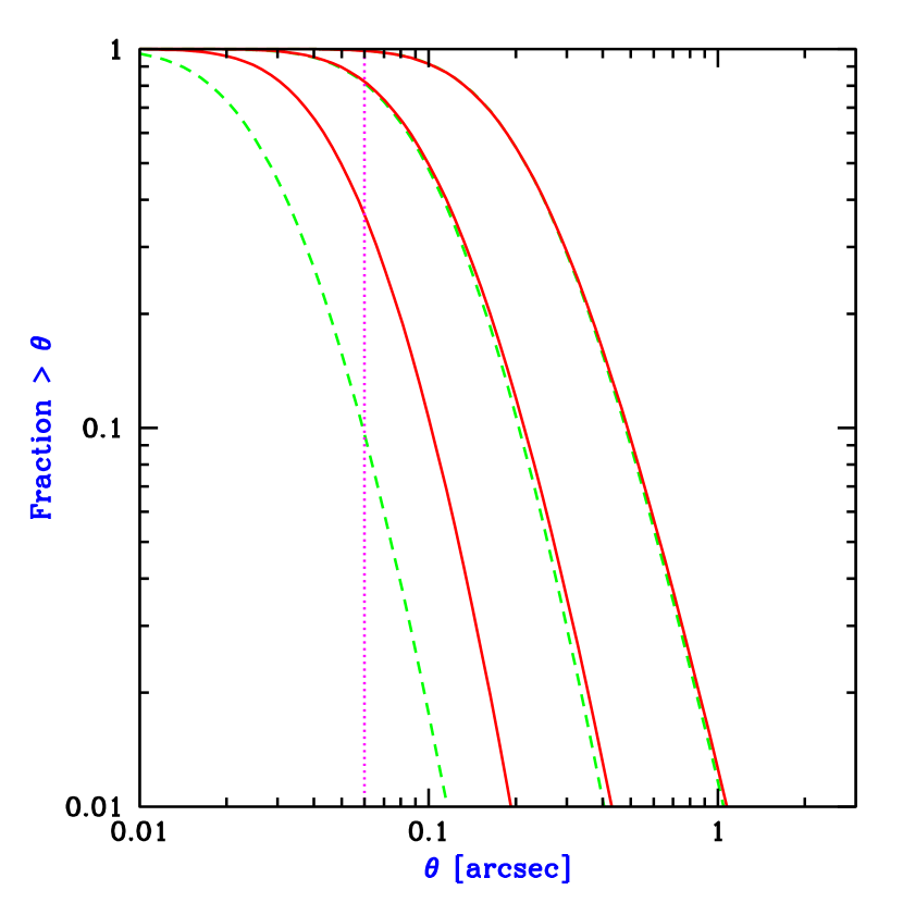
Figure 38: Distribution of galactic disk sizes at various redshifts, in the $\Lambda$CDM model (with parameters given at the end of §1), adopted and modified from Figure 6 of Barkana & Loeb (2000a). Given $\theta$ in arcseconds, each curve shows the fraction of the total number counts contributed by sources larger than $\theta$. The diameter $\theta$ is measured out to one exponential scale length. We show three pairs of curves, at $z=2$, $z=5$ and $z=10$ (from right to left). Each pair includes the distribution for all galaxies (dashed line), and for galaxies detectable by NGST  (solid line) with a limiting point source flux of 0.25 nJy and with an efficiency $\eta=10\%$ assumed for the galaxies. The vertical dotted line indicates the expected NGST  resolution of $0\farcs 06$.

Among detectable galaxies, the typical diameter decreases from $0\farcs 22$ at $z=2$ to $0\farcs 10$ at $z=5$ and $0\farcs 05$ at $z=10$. Note that in $\Lambda$CDM (with ${\Omega_{m}}=0.3$) the angular diameter distance (in units of $c/H_{0}$) actually decreases from 0.40 at $z=2$ to 0.30 at $z=5$ and 0.20 at $z=10$. Galaxies are still typically smaller at the higher redshifts because a halo of a given mass is denser, and thus smaller, at higher redshift, and furthermore the typical halo mass is larger at low redshift due to the growth of cosmic structure with time. At $z=10$, the distribution of detectable galaxies is biased, relative to the distribution of all galaxies, toward large galaxies, since NGST  can only detect the brightest galaxies. The brightest galaxies tend to lie in the most massive and therefore largest halos, and this trend dominates over the higher detection threshold needed for an extended source compared to a point source (§8.1).

Clearly, the angular resolution of NGST  will be sufficiently high to resolve most galaxies. For example, NGST  should resolve approximately $35\%$ of $z=10$ galaxies, $80\%$ of $z=5$ galaxies, and all but $1\%$ of $z=2$ galaxies. This implies that the shapes of these high-redshift galaxies can be studied with NGST.  It also means that the high resolution of NGST  is crucial in making the majority of sources on the sky useful for weak lensing studies (although a mosaic of images is required for good statistics; see also the following subsection).

8.4 Gravitational Lensing

Detailed studies of gravitational lenses have provided a wealth of information on galaxies, both through modeling of individual lens systems (e.g., Schneider, Ehlers, & Falco 1992; Blandford & Narayan 1992) and from the statistical properties of multiply imaged sources (e.g., Turner, Ostriker, & Gott 1984; Maoz & Rix 1993; Kochanek 1996).

The ability to observe large numbers of high-redshift objects promises to greatly extend gravitational lensing studies. Due to the increased path length along the line of sight to the most distant sources, their probability for being lensed is expected to be the highest among all possible sources. Sources at $z>10$ will often be lensed by $z>2$ galaxies, whose masses can then be determined with lens modeling. Similarly, the shape distortions (or weak lensing) caused by foreground clusters of galaxies will be used to determine the mass distributions of less massive and higher redshift clusters than currently feasible. In addition, it will be fruitful to exploit the magnification of the sources to resolve and study more distant galaxies than otherwise possible.

These applications have been explored by Schneider & Kneib (1998), who investigated weak lensing, and by Barkana & Loeb (2000a), who focused on strong lensing. Schneider & Kneib (1998) noted that the ability of NGST  to take deeper exposures than is possible with current instruments will increase the observed density of sources on the sky, particularly of those at high redshifts. The large increase (by $\sim 2$ orders of magnitude over current surveys) may allow such applications as a detailed weak lensing mapping of substructure in clusters. Obviously, the source galaxies must be well resolved to allow an accurate shape measurement. Barkana & Loeb (2000a) estimated the size distribution of galactic disks (see §8.3) and showed that with its expected $\sim 0\farcs 06$ resolution, NGST  should resolve most galaxies even at $z\sim 10$.

The probability for strong gravitational lensing depends on the abundance of lenses, their mass profiles, and the angular diameter distances among the source, the lens and the observer. The statistics of existing lens surveys have been used at low redshifts to constrain the cosmological constant (for the most detailed work see Kochanek 1996, and references therein), although substantial uncertainties remain regarding the luminosity function of early-type galaxies and their dark matter content. Given the early stage of observations of the redshift evolution of galaxies and their dark halos, a theoretical approach based on the Press-Schechter mass function can be used to estimate the lensing rate. This approach has been used in the past for calculating lensing statistics at low redshifts, with an emphasis on lenses with image separations above $5\arcsec$ (Narayan & White 1988; Kochanek 1995; Maoz et al. 1997; Nakamura & Suto 1997; Phillips, Browne, & Wilkinson 2001; Ofek et al. 2001) or on the lensing rates of supernovae (Porciani & Madau 2000; Marri et al. 2000).

The probability for producing multiple images of a source at a redshift $z_{S}$, due to gravitational lensing by lenses with density distributed as in a singular isothermal sphere, is obtained by integrating over lens redshift $z_{L}$ the differential optical depth (Turner, Ostriker, & Gott 1984; Fukugita et al. 1992)

$$d\tau=16\pi^{3}n\left(\frac{\sigma}{c}\right)^{4}(1+z_{L})^{3}\left(\frac{D_{OL}D_{LS}}{D_{OS}}\right)^{2}\frac{cdt}{dz_{L}}dz_{L}\ ,$$ (105)

in terms of the comoving density of lenses $n$, velocity dispersion $\sigma$, look-back time $t$, and angular diameter distances $D$ among the observer, lens and source. More generally we replace $n\sigma^{4}$ by

$$\langle n\sigma^{4}\rangle=\int\frac{dn(M,z_{L})}{dM}\,\sigma^{4}(M,z_{L})\,dM\ ,$$ (106)

where $dn/dM$ is the Press-Schechter halo mass function. It is assumed that $\sigma(M,z)=V_{c}(M,z)/\sqrt{2}$  and that the circular velocity $V_{c}(M,z)$ corresponding to a halo of a given mass is given by equation (25).

The $\Lambda$CDM model (with ${\Omega_{m}}=0.3$) yields a lensing optical depth (Barkana & Loeb 2000a) of $\sim 1\%$ for sources at $z_{S}=10$. The fraction of lensed sources in an actual survey is enhanced, however, by the so-called magnification bias. At a given observed flux level, unlensed sources compete with lensed sources that are intrinsically fainter. Since fainter galaxies are more numerous, the fraction of lenses in an observed sample is larger than the optical depth value given above. The expected slope of the luminosity function of the early sources (§8.2) suggests an additional magnification bias of order 5, bringing the fraction of lensed sources at $z_{S}=10$ to $\sim 5\%$. The lensed fraction decreases to $\sim 3\%$ at $z=5$. With the magnification bias estimated separately for each source population, the expected number of detected multiply-imaged sources per field of view of NGST  (which we assume to be $4\arcmin\times 4\arcmin$) is roughly 5 for $z>10$ quasars, 10 for $z>5$ quasars, 10 for $z>10$ galaxies, and 100 for $z>5$ galaxies.

High-redshift sources will tend to be lensed by galaxies at relatively high redshifts. In Figure 39 (adopted from Figure 2 of Barkana & Loeb 2000a) we show the lens redshift probability density $p(z_{L})$, defined so that the fraction of lenses between $z_{L}$ and $z_{L}+dz_{L}$ is $p(z_{L})dz_{L}$. We consider a source at $z_{S}=5$ (solid curve) or at $z_{S}=10$ (dashed curve). The curves peak around $z_{L}=1$, but in each case a significant fraction of the lenses are above redshift 2: $20\%$ for $z_{S}=5$ and $36\%$ for $z_{S}=10$.

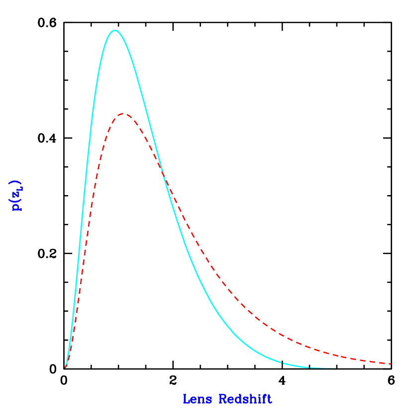
Figure 39: Distribution of lens redshifts for a fixed source redshift, for Press-Schechter halos in $\Lambda$CDM with ${\Omega_{m}}=0.3$ (adopted from Figure 2 of Barkana & Loeb 2000a). Shown for a source at $z_{S}=5$ (solid curve) and for $z_{S}=10$ (dashed curve). The probability density $p(z_{L})$ is shown, where the fraction of lenses between $z_{L}$ and $z_{L}+dz_{L}$ is $p(z_{L})dz_{L}$.

The multiple images of lensed high-redshift sources should be easily resolvable. Indeed, image separations are typically reduced by a factor of only 2–3 between $z_{S}=2$ and $z_{S}=10$, with the reduction almost entirely due to redshift evolution in the characteristic mass of the lenses. With a typical separation of 0.5–1$\arcsec$ for $z_{S}=10$, a large majority of lenses should be resolved given the NGST  resolution of $\sim 0\farcs 06$.

Lensed sources may be difficult to detect if their images overlap the lensing galaxy, and if the lensing galaxy has a higher surface brightness. Although the surface brightness of a background source will typically be somewhat lower than that of the foreground lens (Barkana & Loeb 2000a), the lensed images should be detectable since (i) the image center will typically be some distance from the lens center, of order half the image separation, and (ii) the younger stellar population and higher redshift of the source will make its colors different from those of the lens galaxy, permitting an easy separation of the two in multi-color observations. These helpful features are evident in the currently known systems which feature galaxy-galaxy strong lensing. These include two four-image ‘Einstein cross’ gravitational lenses and other lens candidates discovered by Ratnatunga et al. (1999) in the Hubble Space Telescope  Medium Deep Survey, and a lensed three-image arc detected in the Hubble Deep Field South and studied in detail by Barkana et al. (1999).

9 Observational Probes of the Epoch of Reionization

9.1 Spectral Methods of Inferring the Reionization Redshift

9.1.1 Cosmology with Ly$\alpha$ Photons

The scattering cross-section of the Ly$\alpha$ resonance line by neutral hydrogen is given by (§23 of Peebles 1993)

$$\sigma_{\alpha}(\nu)={3\lambda_{\alpha}^{2}\Lambda_{\alpha}^{2}\over 8\pi}{(\nu/\nu_{\alpha})^{4}\over 4\pi^{2}(\nu-\nu_{\alpha})^{2}+(\Lambda_{\alpha}^{2}/4)(\nu/\nu_{\alpha})^{6}},$$ (107)

where $\Lambda_{\alpha}=(8\pi^{2}e^{2}f_{\alpha}/3m_{e}c\lambda_{\alpha}^{2})=6.25\times 10^{8}~{}{\rm s^{-1}}$ is the Ly$\alpha$ ($2p\rightarrow 1s$) decay rate, $f_{\alpha}=0.4162$ is the oscillator strength, and $\lambda_{\alpha}=1216$Å  and $\nu_{\alpha}=(c/\lambda_{\alpha})=2.47\times 10^{15}~{}{\rm Hz}$ are the wavelength and frequency of the Ly$\alpha$ line. The term in the numerator is responsible for the classical Rayleigh scattering.

We consider a source at a redshift $z_{s}$ beyond the redshift of reionization $z_{\rm reion}$, and the corresponding scattering optical depth of a uniform, neutral IGM of hydrogen density $n_{\rm H,0}(1+z)^{3}$ between the source and the reionization redshift. The optical depth is a function of the observed wavelength $\lambda_{\rm obs}$,

$$\tau(\lambda_{\rm obs})=\int_{z_{\rm reion}}^{z_{s}}dz{cdt\over dz}n_{\rm H,0}(1+z)^{3}\sigma_{\alpha}\left[\nu_{\rm obs}(1+z)\right],$$ (108)

where $\nu_{\rm obs}=c/\lambda_{\rm obs}$ and

$${dt\over dz}=\left[(1+z)H(z)\right]^{-1}=H_{0}^{-1}\left[\Omega_{m}(1+z)^{5}+\Omega_{\Lambda}(1+z)^{2}+(1-\Omega_{m}-\Omega_{\Lambda})(1+z)^{4}\right]^{-1/2}.$$ (109)

At wavelengths longer than Ly$\alpha$ at the source, the optical depth obtains a small value; these photons redshift away from the line center along its red wing and never resonate with the line core on their way to the observer. Considering only the regime in which $|\nu-\nu_{\alpha}|\gg\Lambda_{\alpha}$, we may ignore the second term in the denominator of equation (107). This leads to an analytical result for the red damping wing of the Gunn-Peterson trough (Miralda-Escudé 1998)

$$\tau(\lambda_{\rm obs})=\tau_{s}\left(\Lambda\over 4\pi^{2}\nu_{\alpha}\right){\tilde{\lambda}}_{\rm obs}^{3/2}\left[I({\tilde{\lambda}}_{\rm obs}^{-1})-I([(1+z_{\rm reion})/(1+z_{s})]{\tilde{\lambda}}_{\rm obs}^{-1})\right]~{}~{}~{}~{}~{}~{}{\rm for}~{}~{}{\tilde{\lambda}}_{\rm obs}\geq 1~{},$$ (110)

where $\tau_{s}$ is given in equation (1), and we also define

$${\tilde{\lambda}}_{\rm obs}\equiv{\lambda_{\rm obs}\over(1+z_{s})\lambda_{\alpha}}$$ (111)

and

$$I(x)\equiv{x^{9/2}\over 1-x}+{9\over 7}x^{7/2}+{9\over 5}x^{5/2}+3x^{3/2}+9x^{1/2}-{9\over 2}\ln\left[{1+x^{1/2}\over 1-x^{1/2}}\right]\ .$$ (112)

At wavelengths corresponding to the Ly$\alpha$ resonance between the source redshift and the reionization redshift, $(1+z_{\rm reion})\lambda_{\alpha}\leq\lambda_{\rm obs}\leq(1+z_{s})\lambda_{\alpha}$, the optical depth is given by equation (1). Since $\tau_{s}\sim 10^{5}$, the flux from the source is entirely suppressed in this regime. Similarly, the Ly$\beta$ resonance produces another trough at wavelengths $(1+z_{\rm reion})\lambda_{\beta}\leq\lambda\leq(1+z_{s})\lambda_{\beta}$, where $\lambda_{\beta}=(27/32)\lambda_{\alpha}=1026\,$Å, and the same applies to the higher Lyman series lines. If $(1+z_{s})\geq 1.18(1+z_{\rm reion})$ then the Ly$\alpha$ and the Ly$\beta$ resonances overlap and no flux is transmitted in-between the two troughs (see Figure 40). The same holds for the higher Lyman-series resonances down to the Lyman limit wavelength of $\lambda_{c}=912$Å.

At wavelengths shorter than $\lambda_{c}$, the photons are absorbed when they photoionize atoms of hydrogen or helium. The bound-free absorption cross-section from the ground state of a hydrogenic ion with nuclear charge $Z$ and an ionization threshold $h\nu_{0}$, is given by (Osterbrock 1974),

$$\sigma_{bf}(\nu)={6.30\times 10^{-18}\over Z^{2}}~{}{\rm cm^{2}}\times\left({\nu_{0}\over\nu}\right)^{4}{e^{4-(4\tan^{-1}\epsilon)/\epsilon}\over 1-e^{-2\pi/\epsilon}}~{}~{}~{}~{}~{}{\rm for}~{}~{}\nu\geq\nu_{0},$$ (113)

where

$$\epsilon\equiv\sqrt{{\nu\over\nu_{0}}-1}.$$ (114)

For neutral hydrogen, $Z=1$ and $\nu_{{\rm H},0}=(c/\lambda_{c})=3.29\times 10^{15}$ Hz ($h\nu_{\rm H,0}=13.60$ eV); for singly-ionized helium, $Z=2$ and $\nu_{\rm He~{}II,0}=1.31\times 10^{16}~{}{\rm Hz}$ ($h\nu_{\rm He~{}II,0}=54.42$ eV). The cross-section for neutral helium is more complicated; when averaged over its narrow resonances it can be fitted to an accuracy of a few percent up to $h\nu=50$ keV by the fitting function (Verner et al. 1996)

$$\sigma_{bf,{\rm He~{}I}}(\nu)=9.492\times 10^{-16}~{}{\rm cm^{2}}\,\times\left[(x-1)^{2}+4.158\right]y^{-1.953}\left(1+0.825y^{1/4}\right)^{-3.188},$$ (115)

where $x\equiv[(\nu/3.286\times 10^{15}~{}{\rm Hz})-0.4434]$, $y\equiv x^{2}+4.563$, and the threshold for ionization is $\nu_{\rm He~{}I,0}=5.938\times 10^{15}~{}{\rm Hz}$ ($h\nu_{\rm He~{}I,0}=24.59$ eV).

For rough estimates, the average photoionization cross-section for a mixture of hydrogen and helium with cosmic abundances can be approximated in the range of $54<h\nu\lesssim 10^{3}$ eV as $\sigma_{bf}\approx\sigma_{0}(\nu/\nu_{\rm H,0})^{-3}$, where $\sigma_{0}\approx 6\times 10^{-17}~{}{\rm cm^{2}}$ (Miralda-Escudé 2000). The redshift factor in the cross-section then cancels exactly the redshift evolution of the gas density and the resulting optical depth depends only on the elapsed cosmic time, $t(z_{\rm reion})-t(z_{s})$. At high redshifts (equations (9) and (10) in §2.1) this yields,

$$\tau_{bf}(\lambda_{\rm obs}) = \int_{z_{\rm reion}}^{z_{s}}dz{cdt\over dz}n_{0}(1+z)^{3}\sigma_{\rm bf}\left[\nu_{\rm obs}(1+z)\right]$$ (116)

$$\approx 1.5\times 10^{2}\left({\Omega_{b}h\over 0.03}\right)\left({\Omega_{m}\over 0.3}\right)^{-1/2}\left({\lambda\over 100{\rm\AA}}\right)^{3}\left[{1\over(1+z_{\rm reion})^{3/2}}-{1\over(1+z_{s})^{3/2}}\right].$$

The bound-free optical depth only becomes of order unity in the extreme UV to soft X-rays, around $h\nu\sim 0.1$ keV, a regime which is unfortunately difficult to observe due to Galactic absorption (Miralda-Escudé 2000).

A sketch of the overall spectrum of a source slightly above the reionization redshift, i.e., with $1<[(1+z_{\rm s})/(1+z_{\rm reion})]<1.18$, is shown in Figure 40. The transmitted flux between the Gunn-Peterson troughs due to Ly$\alpha$ and Ly$\beta$ absorption is suppressed by the Ly$\alpha$ forest in the post-reionization epoch. Transmission of flux due to H 2 bubbles in the pre-reionization epoch is expected to be negligible (Miralda-Escudé 1998). The redshift of reionization can be inferred in principle from the spectral shape of the red damping wing (Miralda-Escudé & Rees 1998; Miralda-Escudé 1998) or from the transmitted flux between the Lyman series lines (Haiman & Loeb 1999a). However, these signatures are complicated in reality by damped Ly$\alpha$ systems along the line of sight or by the inhomogeneity or peculiar velocity field of the IGM in the vicinity of the source. Moreover, bright sources, such as quasars, tend to ionize their surrounding environment (Wood & Loeb 2000) and the resulting H 2 region in the IGM could shift the Ly$\alpha$ trough substantially (Cen & Haiman 2000; Madau & Rees 2000).

The inference of the Ly$\alpha$ transmission properties of the IGM from the observed spectrum of high-redshift sources suffers from uncertainties about the precise emission spectrum of these sources, and in particular the shape of their Ly$\alpha$ emission line. The first galaxies and quasars are expected to have pronounced recombination lines of hydrogen and helium due to the lack of dust in their interstellar medium (see §4.1.3 for more details). Lines such as $H_{\alpha}$ or the He 2 1640 Å  line should reach the observer unaffected by the intervening IGM, since their wavelength is longer than that of the Ly$\alpha$ transition which dominates the IGM opacity (Oh 1999). However, as described above, the situation is different for the Ly$\alpha$ line photons from the source. As long as $z_{s}>z_{\rm reion}$, the intervening neutral IGM acts like a fog and obscures the view of the Ly$\alpha$ line itself [in contrast to the situation with sources at $z_{s}<z_{\rm reion}$, where most of the intervening IGM is ionized and only photons more energetic than Ly$\alpha$ are suppressed by the Ly$\alpha$ forest (see Figure 3)]. Photons which are emitted at the Ly$\alpha$ line center have an initial scattering optical depth of $\sim 10^{5}$ in the surrounding medium.

The Ly$\alpha$ line photons are not destroyed but instead are absorbed and re-emitted. Due to the Hubble expansion of the IGM around the source, the frequency of the photons is slightly shifted by the Doppler effect in each scattering event. As a result, the photons diffuse in frequency to the red side of the Ly$\alpha$ resonance. Eventually, when their net frequency redshift is sufficiently large, they escape and travel freely towards the observer (see Figure 41). As a result, the source creates a faint Ly$\alpha$ halo on the sky. The well-defined radiative transfer problem of a point source of Ly$\alpha$ photons embedded in a uniform, expanding neutral IGM was solved by Loeb & Rybicki (1999). The Ly$\alpha$ halo can be simply characterized by the frequency redshift relative to the line center, $(\nu-\nu_{\alpha})$, which is required in order to make the optical depth from the source [equation (110)] equal to unity. At high redshifts, the leading term in equation (110) yields

$$\nu_{\star}=8.85\times 10^{12}~{}{\rm Hz}\times\left({\Omega_{b}h\over 0.05\sqrt{\Omega_{m}}}\right)\left(1+z_{s}\over 10\right)^{3/2}.$$ (117)

This is the frequency interval over which the damping wing affects the source spectrum. A frequency shift of $\nu_{\star}=8.85\times 10^{12}$ Hz relative to the line center corresponds to a fractional shift of $(\nu_{\star}/\nu_{\alpha})=(v/c)=3.6\times 10^{-3}$ or a Doppler velocity of $v\sim 10^{3}~{}{\rm km~{}s^{-1}}$. The halo size is then defined by the corresponding proper distance from the source at which the Hubble velocity provides a Doppler shift of this magnitude,

$$r_{\star}=1.1\left({\Omega_{b}/0.05\over\Omega_{m}/0.3}\right)~{}{\rm Mpc}.$$ (118)

Typically, the Ly$\alpha$ halo of a source at $z_{\rm s}\sim 10$ occupies an angular radius of $\sim 15^{\prime\prime}$ on the sky and yields an asymmetric line profile as shown in Figures 41 and 42. The scattered photons are highly polarized and so the shape of the halo would be different if viewed through a polarization filter (Rybicki & Loeb 1999).

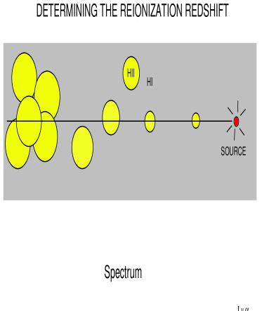
Figure 40: Sketch of the expected spectrum of a source at a redshift $z_{s}$ slightly above the reionization redshift $z_{\rm reion}$. The transmitted flux due to H 2 bubbles in the pre-reionization era and the Ly$\alpha$ forest in the post-reionization era is exaggerated for illustration.

Figure 41: Loeb-Rybicki halos: Scattering of Ly$\alpha$ line photons from a galaxy embedded in the neutral IGM prior to reionization. The line photons diffuse in frequency due to the Hubble expansion of the surrounding medium and eventually redshift out of resonance and escape to infinity. A distant observer sees a Ly$\alpha$ halo surrounding the source, along with a characteristically asymmetric line profile. The observed line should be broadened and redshifted by about one thousand ${\rm km~{}s^{-1}}$ relative to other lines (such as H_α) emitted by the galaxy.

Figure 42: Monochromatic photon luminosity of a Ly$\alpha$ halo as a function of frequency redshift, ${\tilde{\nu}}\equiv(\nu_{\alpha}-\nu)/\nu_{\star}$. The observed spectral flux of photons $F(\nu)$ (in photons cm^-2 s^-1 Hz^-1) from the entire Ly$\alpha$ halo is $F(\nu)=({{\tilde{L}}({\tilde{\nu}})/4\pi d_{\rm L}^{2}})({{\dot{N}_{\alpha}}/\nu_{\star}})(1+z_{s})^{2}$ where ${\dot{N}_{\alpha}}$ is the production rate of Ly$\alpha$ photons by the source (in ${\rm photons~{}s^{-1}}$), $\nu={\tilde{\nu}}\nu_{\star}/(1+z_{\rm s})$, and $d_{\rm L}$ is the standard luminosity distance to the source (from Loeb & Rybicki 1999).

Detection of the diffuse Ly$\alpha$ halos around bright high-redshift sources (which are sufficiently rare so that their halos do not overlap) would provide a unique tool for probing the distribution and the velocity field of the neutral IGM before the epoch of reionization. The Ly$\alpha$ sources serve as lamp posts which illuminate the surrounding H 1 fog. On sufficiently large scales where the Hubble flow is smooth and the gas is neutral, the Ly$\alpha$ brightness distribution can be used to determine the cosmological mass densities of baryons and matter. Due to their low surface brightness, the detection of Ly$\alpha$ halos through a narrow-band filter is much more challenging than direct observation of their sources at somewhat longer wavelengths. However, NGST  might be able to detect the Ly$\alpha$ halos around sources as bright as the quasar discovered by Fan et al. (2000) at $z=5.8$ or the galaxy discovered by Hu et al. (1999) at $z=5.74$, even if these sources were moved out to $z\sim 10$ (see §4 in Loeb & Rybicki 1999). The disappearance of Ly$\alpha$ halos below a certain redshift can be used to determine $z_{\rm reion}$.

9.1.2 21 cm Tomography of the Reionization Epoch

The ground state of hydrogen exhibits hyperfine splitting involving the spins of the proton and the electron. The state with parallel spins (the triplet state) has a slightly higher energy than the state with anti-parallel spins (the singlet state). The 21 cm line associated with the spin-flip transition from the triplet to the singlet state is often used to detect neutral hydrogen in the local universe. At high redshift, the occurrence of a neutral pre-reionization IGM offers the prospect of detecting the first sources of radiation and probing the reionization era by mapping the 21 cm emission from neutral regions. While its energy density is estimated to be only a $1\%$ correction to that of the CMB, the redshifted 21 cm emission should display angular structure as well as frequency structure due to inhomogeneities in the gas density field (Hogan & Rees 1979; Scott & Rees 1990), hydrogen ionized fraction, and spin temperature (Madau, Meiksin, & Rees 1997). Some of the resulting signatures during the pre-overlap phase of reionization (§6.3.1) and during the overlap phase are discussed by Tozzi et al. (2000) and Shaver et al. (1999), respectively. Also, the 21 cm signatures have been explored in a numerical simulation by Gnedin & Ostriker (1997). Indeed, a full mapping of the distribution of H 1 as a function of redshift is possible in principle. Although detecting the presence of the largest H 2 regions may be within the reach of proposed instruments such as the Square Kilometer Array (hereafter SKA; see Taylor & Braun 1999), these instruments may not have sufficient sensitivity at the sub-arcminute resolution that would be necessary for a detailed mapping. Moreover, serious technical challenges and problems due to foreground contamination must be overcome even for an initial detection of the reionization signal.

The basic physics of the hydrogen spin transition is determined as follows (for a more detailed treatment, see Madau et al. 1997). The ground-state hyperfine levels of hydrogen tend to thermalize with the CMB background, making the IGM unobservable. If other processes shift the hyperfine level populations away from thermal equilibrium, then the gas becomes observable against the CMB in emission or in absorption. The relative occupancy of the spin levels is usually described in terms of the hydrogen spin temperature $T_{S}$, defined by

$$\frac{n_{1}}{n_{0}}=3\,\exp\left\{-\frac{T_{*}}{T_{S}}\right\}\,$$ (119)

where $n_{0}$ and $n_{1}$ are the singlet and triplet hyperfine levels in the atomic ground state ($n=1$), and $T_{*}=0.07$ K is defined by $k_{B}T_{*}=E_{21}$, where the energy of the 21 cm transition is $E_{21}=5.9\times 10^{-6}$ eV, corresponding to a frequency of 1420 MHz. In the presence of the CMB alone, the spin states reach thermal equilibrium with $T_{S}=T_{\rm CMB}=2.73(1+z)$ K on a time-scale of $T_{*}/(T_{\rm CMB}A_{10})\simeq 3\times 10^{5}(1+z)^{-1}$ yr, where $A_{10}=2.9\times 10^{-15}$ s^-1 is the spontaneous decay rate of the hyperfine transition. This time-scale is much shorter than the age of the universe at all redshifts after cosmological recombination.

The IGM is observable when the kinetic temperature $T_{K}$ of the gas differs from $T_{\rm CMB}$ and an effective mechanism couples $T_{S}$ to $T_{K}$. Although collisional de-excitation of the triplet level (Purcell & Field 1956) is a possible mechanism, in the low-density IGM the dominant mechanism is scattering by Ly$\alpha$ photons (Wouthuysen 1952; Field 1958). Continuum UV photons produced by early radiation sources redshift by the Hubble expansion into the local Ly$\alpha$ line at a lower redshift. These photons mix the spin states via the Wouthuysen-Field process whereby an atom initially in the $n=1$ state absorbs a Ly$\alpha$ photon, and the spontaneous decay which returns it from $n=2$ to $n=1$ can result in a final spin state which is different from the initial one. Since the neutral IGM is highly opaque to resonant scattering, the shape of the radiation spectrum near Ly$\alpha$ is determined by $T_{K}$ (Field 1959), and the spin temperature is then a weighed mean of $T_{K}$ and $T_{\rm CMB}$:

$$T_{S}=\frac{T_{\rm CMB}+y_{\alpha}T_{K}}{1+y_{\alpha}}\ ,$$ (120)

where (if $T_{S}\gg T_{*}$) the Ly$\alpha$ pumping efficiency is

$$y_{\alpha}=\frac{P_{10}T_{*}}{A_{10}T_{K}}\ .$$ (121)

Here $P_{10}$ is the indirect de-excitation rate of the triplet $n=1$ state via the Wouthuysen-Field process, related to the total scattering rate $P_{\alpha}$ of Ly$\alpha$ photons by $P_{10}=4P_{\alpha}/27$ (Field 1958). Thus the critical value of $P_{\alpha}$ is given by the thermalization rate (Madau et al. 1997)

$$P_{\rm th}\equiv\frac{27A_{10}T_{\rm CMB}}{4T_{*}}\simeq 7.6\times 10^{-12}\,\left(\frac{1+z}{10}\right)\ {\rm s}^{-1}\ .$$ (122)

A patch of neutral hydrogen at the mean density and with a uniform $T_{S}$ produces an optical depth at $21(1+z)$ cm of

$$\tau(z)=9.0\times 10^{-3}\left(\frac{T_{\rm CMB}}{T_{S}}\right)\left(\frac{\Omega_{b}h}{0.03}\right)\left(\frac{{\Omega_{m}}}{0.3}\right)^{-1/2}\left(\frac{1+z}{10}\right)^{1/2}\ ,$$ (123)

assuming a high redshift $z$. Since the brightness temperature through the IGM is $T_{b}=T_{\rm CMB}e^{-\tau}+T_{S}(1-e^{-\tau})$, the observed differential antenna temperature of this region relative to the CMB is (Madau et al. 1997, with the ${\Omega_{m}}$ dependence added)

$$\delta T_{b}=(1+z)^{-1}(T_{S}-T_{\rm CMB})(1-e^{-\tau})\simeq 25\,{\rm mK}\,\left(\frac{\Omega_{b}h}{0.03}\right)\left(\frac{{\Omega_{m}}}{0.3}\right)^{-1/2}\left(\frac{1+z}{10}\right)^{1/2}\left(\frac{T_{S}-T_{\rm CMB}}{T_{S}}\right)\ ,$$ (124)

where $\tau\ll 1$ is assumed and $\delta T_{b}$ has been redshifted to redshift zero. In overdense regions, the observed $\delta T_{b}$ is proportional to the overdensity, and in partially ionized regions $\delta T_{b}$ is proportional to the neutral fraction. Thus, if $T_{S}\gg T_{\rm CMB}$ then the IGM is observed in emission at a level that is independent of $T_{S}$. On the other hand, if $T_{S}\ll T_{\rm CMB}$ then the IGM is observed in absorption at a level that is a factor $\sim T_{\rm CMB}/T_{S}$ larger than in emission. As a result, a number of cosmic events are expected to leave observable signatures in the redshifted 21 cm line.

Since the CMB temperature is only $2.73(1+z)$ K, even relatively inefficient heating mechanisms are expected to heat the IGM above $T_{\rm CMB}$ well before reionization. Possible preheating sources include soft X-rays from early quasars or star-forming regions, as well as thermal bremsstrahlung from ionized gas in collapsing halos. However, even the radiation from the first stars may suffice for an early preheating. Only $\sim 10\%$ of the present-day global star formation rate is required (Madau et al. 1997) for a sufficiently strong Ly$\alpha$ background which produces a scattering rate above the thermalization rate $P_{\rm th}$. Such a background drives $T_{S}$ to the kinetic gas temperature, which is initially lower than $T_{\rm CMB}$ because of adiabatic expansion. Thus, the entire IGM can be seen in absorption, but the IGM is then heated above $T_{\rm CMB}$ in $\sim 10^{8}$ yr (Madau et al. 1997) by the atomic recoil in the repeated resonant Ly$\alpha$ scattering. According to §8.1 (also compare Gnedin 2000a), the required level of star formation is expected to be reached already at $z\sim 20$, with the entire IGM heated well above the CMB by the time overlap begins at $z\sim 10$. Thus, although the initial absorption signal is in principle detectable with the SKA (Tozzi et al. 2000), it likely occurs at $\lesssim 100$ MHz where Earth-based radio interference is highly problematic.

As individual ionizing sources turn on in the pre-overlap stage of reionization, the resulting H 2 bubbles may be individually detectable if they are produced by rare and luminous sources such as quasars. If the H 2 region expands into an otherwise unperturbed IGM, then the expanding shell can be mapped as follows (Tozzi et al. 2000). The H 2 region itself, of course, shows neither emission nor absorption. Outside the ionized bubble, a thin shell of neutral gas is heated above the CMB temperature and shows up in emission. A much thicker outer shell is cooler than the CMB due to adiabatic expansion, but satisfies $T_{S}=T_{K}$ and produces absorption. Finally, at large distances from the quasar, $T_{S}$ approaches $T_{\rm CMB}$ as the quasar radiation weakens. For a quasar with an ionizing intensity of $10^{57}$ photons s^-1 observed after $\sim 10^{7}$ yr with $2\arcmin$ resolution and 1 MHz bandwidth, the signal ranges from -3 to 3 $\mu$Jy per beam (Tozzi et al. 2000). Mapping such regions would convey information on the quasar number density, ionizing intensity, opening angle, and on the density distribution in the surrounding IGM. Note, however, that an H 2 region which forms at a redshift approaching overlap expands into a preheated IGM. In this case, the H 2 region itself still appears as a hole in an otherwise emitting medium, but the quasar-induced heating is not probed, and there is no surrounding region of absorption to supply an enhanced contrast.

At redshifts approaching overlap, the IGM should be almost entirely neutral but with $T_{S}\gg T_{\rm CMB}$. In this redshift range there should still be an interesting signal due to density fluctuations. The same cosmic network of sheets and filaments that gives rise to the Ly$\alpha$ forest observed at $z\lesssim 5$ should lead to fluctuations in the 21 cm brightness temperature at higher redshifts. At 150 MHz ($z=8.5$), for observations with a bandwidth of 1 MHz, the root mean square fluctuation should be $\sim 10$ mK at $1\arcmin$, decreasing with scale (Tozzi et al. 2000).

A further signature, observable over the entire sky, should mark the overlap stage of reionization. During overlap, the IGM is transformed from being a neutral, preheated and thus emitting gas, to being almost completely ionized. This disappearance of the emission over a relatively narrow redshift range can be observed as a drop in the brightness temperature at the frequencies corresponding to the latter stages of overlap (Shaver et al. 1999). This exciting possibility, along with those mentioned above, face serious challenges in terms of signal contamination and calibration. The noise sources include galactic and extragalactic emission sources, as well as terrestrial interference, and all of these foregrounds must be modeled and accurately removed in order to observe the fainter cosmological signal (see Shaver et al. 1999 for a detailed discussion). For the overlap stage in particular, the sharpness of the spectral feature is the key to its detectability, but it may be significantly smoothed by inhomogeneities in the IGM.

9.2 Effect of Reionization on CMB Anisotropies

In standard cosmological models, the early universe was hot and permeated by a nearly uniform radiation bath. At $z\sim 1200$ the free protons and electrons recombined to form hydrogen atoms, and most of the photons last scattered as the scattering cross-section dropped precipitously. These photons, observed today as the Cosmic Microwave Background (CMB), thus yield a snapshot of the state of the universe at that early time. Small fluctuations in the density, velocity, and gravitational potential lead to observed anisotropies (e.g., Sachs & Wolfe 1967; Bennett et al. 1996) that can be analyzed to yield a great wealth of information on the matter content of the universe and on the values of the cosmological parameters (e.g., Hu 1995; Jungman et al. 1996).

Reionization can alter the anisotropy spectrum, by erasing some of the primary anisotropy imprinted at recombination, and by generating additional secondary fluctuations that could be used to probe the era of reionization itself (see Haiman & Knox 1999 for a review). The primary anisotropy is damped since the rescattering leads to a blending of photons from initially different lines of sight. Furthermore, not all the photons scatter at the same time, rather the last scattering surface has a finite thickness. Perturbations on scales smaller than this thickness are damped since photons scattering across many wavelengths give canceling redshifts and blueshifts. If reionization occurs very early, the high electron density produces efficient scattering, and perturbations are damped on all angular scales except for the very largest.

The optical depth to scattering over a proper length $dl$ is $d\tau=\sigma_{T}\,n_{e}\,dl$, where $\sigma_{T}$ is the Thomson cross-section and $n_{e}$ the density of free electrons. If reionization occurs instantaneously at redshift $z$, then the total scattering optical depth in $\Lambda$CDM is given by (e.g., §7.1.1 of Hu 1995)

$$\tau=0.041\frac{\Omega_{b}h}{{\Omega_{m}}}\left\{\left[1-{\Omega_{m}}+{\Omega_{m}}(1+z)^{3}\right]^{1/2}-1\right\}\ .$$ (125)

With our standard parameters (end of §1) this implies $\tau=0.037$ at the current lower limit on reionization of $z=5.8$ (Fan et al. 2000), with $\tau=0.10$ if $z=11.6$ and $\tau=0.15$ if $z=15.3$. Recent observations of small-scale anisotropies (Lange et al. 2000; Balbi et al. 2000) revealed a peak in the power spectrum on a $\sim 1^{\circ}$ scale, as expected from the primary anisotropies in standard cosmological models. This indicates that the reionization damping, if present, is not very large, and the observations set a limit of $\tau<0.33$ at $95\%$ confidence (Tegmark & Zaldarriaga 2000) and, therefore, imply that reionization must have occurred at $z\lesssim 30$.

However, measuring a small $\tau$ from the temperature anisotropies alone is expected to be very difficult since the anisotropy spectrum depends on a large number of other parameters, creating a near-degeneracy which limits our ability to measure each parameter separately; the degeneracy of $\tau$ with other cosmological parameters is due primarily to a degeneracy with the gravitational-wave background. However, Thomson scattering also creates net polarization for incident radiation which has a quadrupole anisotropy. This anisotropy was significant at reionization due to large-scale structure which had already affected the gas distribution. The result is a peak in the polarization power spectrum on large angular scales of order tens of degrees (Zaldarriaga 1997). Although experiments must overcome systematic errors from the detector itself and from polarized foregrounds (such as galactic dust emission and synchrotron radiation), parameter estimation models (Eisenstein, Hu, & Tegmark 1999; Zaldarriaga, Spergel, & Seljak 1997) suggest that the peak can be used to measure even very small values of $\tau$: $2\%$ for the upcoming MAP satellite, and $0.5\%$ for the Planck satellite which will reach smaller angular scales with higher accuracy.

Reionization should also produce additional temperature anisotropies on small scales. These result from the Doppler effect. By the time of reionization, the baryons have begun to follow dark matter potentials and have acquired a bulk velocity. Since the electrons move with respect to the radiation background, photons are given a Doppler kick when they scatter off the electrons. Sunyaev (1978) and Kaiser (1984) showed, however, that a severe cancellation occurs if the electron density is homogeneous. Opposite Doppler shifts on crests and troughs of a velocity perturbation combine to suppress the anisotropy induced by small-scale velocity perturbations. The cancellation is made more severe by the irrotational nature of gravitationally-induced flows. However, if the electron density varies spatially, then the scattering probability is not equal on the crest and on the trough, and the two do not completely cancel. Since a non-zero effect requires variation in both electron density and velocity, it is referred to as a second-order anisotropy.

The electron density can vary due to a spatial variation in either the baryon density or the ionized fraction. The former is referred to as the Ostriker-Vishniac effect (Ostriker & Vishniac 1986; Vishniac 1987). The latter depends on the inhomogeneous topology of reionization, in particular on the size of H 2 regions due to individual sources (§6.2) and on spatial correlations among different regions. Simple models have been used to investigate the character of anisotropies generated during reionization (Gruzinov & Hu 1998; Knox et al. 1998; Aghanim et al. 1996). The Ostriker-Vishniac effect is expected to dominate all anisotropies at small angular scales (e.g., Jaffe & Kamionkowski 1998), below a tenth of a degree, because the primary anisotropies are damped on such small scales by diffusion (Silk damping) and by the finite thickness of the last scattering surface. Anisotropies generated by inhomogeneous reionization may be comparable to the Ostriker-Vishniac effect, and could be detected by MAP and Planck, if reionization is caused by bright quasars with 10 Mpc-size ionized bubbles. However, the smaller bubbles expected for mini-quasars or for star-forming dwarf galaxies would produce an anisotropy signal which is weaker and at smaller angular scales, likely outside the range of the upcoming satellites (see, e.g., Haiman & Knox 1999 for discussion). Gnedin & Jaffe (2000) used a numerical simulation to show that, in the case of stellar reionization, the effect on the CMB of patchy reionization is indeed sub-dominant compared to the contribution of non-linear density and velocity fluctuations. Nevertheless, a signature of reionization could still be detected in future measurements of CMB angular fluctuations on the scale of a few arcseconds (see also Bruscoli et al. 2000, who find a somewhat higher power spectrum due to patchy reionization).

9.3 Remnants of High-Redshift Systems in the Local Universe

At the end of the reionization epoch, the heating of the IGM resulted in the photo-evaporation of gas out of halos of circular velocity $V_{c}$ above $\sim 10$–$15\ {\rm km~{}s^{-1}}$ (§6.4). The pressure of the hot gas subsequently shut off gas infall into even more massive halos, those with $V_{c}\sim 30\ {\rm km~{}s^{-1}}$ (§6.5). Thus, the gas reservoir of photo-evaporating halos could not be immediately replenished. Some dwarf galaxies which were prevented from forming after reionization could have eventually collected gas at $z=1$–2, when the UV background flux declined sufficiently (Babul & Rees 1992; Kepner, Babul, & Spergel 1997). However, Kepner et al. (1997) found that even if the ionizing intensity $J_{21}$ declines as $(1+z)^{4}$ below $z=3$, only halos with $V_{c}\gtrsim 20\ {\rm km\ s}^{-1}$ can form atomic hydrogen by $z=1$, and $V_{c}\gtrsim 25\ {\rm km\ s}^{-1}$ is required to form molecular hydrogen. While the fact that the IGM was reionized has almost certainly influenced the abundance and properties of dwarf galaxies observed today, the exact manifestations of this influence and ways to prove that they occurred have not been well determined. In this section we summarize recent work on this topic, which should remain an active research area.

The suppression of gas infall mentioned above suggests that the abundance of luminous halos as a function of circular velocity should show a break, with a significant drop in the abundance below $V_{c}=30\ {\rm km~{}s^{-1}}$. Such a drop may in fact be required in order to reconcile the $\Lambda$CDM model with observations. Klypin et al. (1999) and Moore et al. (1999) found that the abundance of halos with $V_{c}\sim 10$–$30\ {\rm km~{}s^{-1}}$ in numerical simulations of the Local Group environment is higher by an order of magnitude than the observed dwarf galaxy abundance. The predicted and observed abundances matched well at $V_{c}>50\ {\rm km~{}s^{-1}}$. Bullock et al. (2000a) considered whether photoionization can explain the discrepancy at the low-mass end by preventing dark matter halos from forming stars. They assumed that a sub-halo in the Local Group can host an observable galaxy only if already at reionization its main progenitor contained a fraction $f$ of the final sub-halo mass. Using semi-analytic modeling, they found a close match to the observed circular velocity distribution for $z_{\rm reion}=8$ and $f=0.3$.

These results neglect several complications. As mentioned above, halos with $V_{c}\gtrsim 20\ {\rm km\ s}^{-1}$ may be able to accrete gas and form stars once again at $z\lesssim 1$. Any accreted gas at low redshift could have been previously enriched with metals and molecules, thus enabling more efficient cooling. On the other hand, if the progenitors had a $V_{c}\lesssim 17\ {\rm km~{}s^{-1}}$ at $z_{\rm reion}$ then they were not able to cool and form stars, unless molecular hydrogen had not been dissociated (§3.3). In order to reconcile the photoionization scenario with the recent episodes of star formation deduced to have occurred in most dwarf galaxies (e.g., Mateo 1998; Grebel 1998), a continuous recycling of gas over many generations of stars must be assumed. This would mean that supernova feedback (§7.1) was unable to shut off star formation even in these smallest known galaxies. In addition, the existence of a large abundance of sub-halos may be problematic even if the sub-halos have no gas, since they would interact with the disk dynamically and tend to thicken it (Toth & Ostriker 1992; Moore et al. 1999; Velazquez & White 1999).

However, the photoionization scenario is useful because it may be testable through other implications. For example, Bullock et al. (2001) used semi-analytic modeling to show that many subhalos which did form stars before reionization were tidally disrupted in the Milky Way’s gravitational field, and the resulting stellar streams may be observable. The formation of the Milky Way’s stellar component has also been investigated by White & Springel (1999). They combined a scaled-down dark matter cluster simulation with semi-analytic prescriptions for star formation in halos, and showed that the oldest stars in the Milky Way should be located mostly in the inner halo or bulge, but they cannot be easily identified because the populations of old stars and of low metallicity stars are only weakly correlated.

Gnedin (2000c) pointed out several observed features of dwarf galaxies that may be related to their high-redshift histories. First, almost all Local Group dwarf galaxies with measured star formation histories show a sharp decline in the star formation rate around 10 Gyr ago. Gnedin noted that this drop could correspond to the suppression of star formation due to reionization (§6.5) if the measured ages of the old stellar populations are somewhat underestimated; or that it could instead correspond to the additional suppression caused by helium reionization (§6.3.2) at $z\gtrsim 3$. He showed that if only the old stellar population is considered, then the Schmidt Law (§5.2) implies that the luminosity of each dwarf galaxy, divided by a characteristic volume containing a fixed fraction of all the old stars, should be proportional to some power of the central luminosity density. This assumes that the present central luminosity density of old stars is a good measure of the original gas density, i.e., that in the core almost all the gas was transformed into stars, and feedback did not play a role. It also assumes that the gas density distribution was self-similar in all the dwarf galaxies during the period when they formed stars, and that the length of this period was also the same in all galaxies. These assumptions are required in order for the total stellar content of each galaxy to be simply related to the central density via the Schmidt Law evaluated at the center. Taking ten galaxies which have well-measured star formation histories, and which formed most of their stars more than 10 Gyr ago, Gnedin found a correlation with a power law of $3/2$, as expected from the Schmidt Law (§5.2). Clearly, the theoretical derivation of this correlation combines many simplistic assumptions. However, explaining the observed correlation is a challenge for any competing models, e.g., models where feedback plays a dominant role in regulating star formation.

Barkana & Loeb (1999) noted that a particularly acute puzzle is presented by the very smallest galaxies, the nine dwarf spheroidals in the Local Group with central velocity dispersions $\sigma\lesssim 10\ {\rm km\ s}^{-1}$, including five below $7\ {\rm km\ s}^{-1}$ (see recent reviews by Mateo 1998 & van den Bergh 2000). These galaxies contain old stars that must have formed at $z\gtrsim 2$, before the ionizing background dropped sufficiently to allow them to form. There are several possible solutions to the puzzle of how these stars formed in such small halos or in their progenitors which likely had even smaller velocity dispersions. The solutions are that (i) molecular hydrogen allowed these stars to form at $z>z_{\rm reion}$, as noted above, (ii) the measured stellar velocity dispersions of the dwarf galaxies are well below the velocity dispersions of their dark matter halos, or (iii) the dwarf galaxies did not form via the usual hierarchical scenario.

One major uncertainty in comparing observations to hierarchical models is the possibility that the measured velocity dispersion of stars in the dwarf spheroidals underestimates the velocity dispersion of their dark halos. Assuming that the stars are in equilibrium, their velocity dispersion could be lower than that of the halo if the mass profile is shallower than isothermal beyond the stellar core. The velocity dispersion and mass-to-light ratio of a dwarf spheroidal could also appear high if the galaxy is non-spherical or the stellar orbits are anisotropic. The observed properties of dwarf spheroidals require a central mass density of order $0.1M_{\sun}$ pc^-3 (e.g., Mateo 1998), which is $\sim 7\times 10^{5}$ times the present critical density. Thus, only the very inner parts of the halos are sampled by the central velocity dispersion. Detailed observations of the velocity dispersion profiles of these galaxies could be used to determine the circular velocity of the underlying halo more reliably.

A cosmological scenario for the formation of dwarf spheroidal galaxies is favored by the fact that they are observed to be dark matter dominated, but this may not rule out all the alternatives. The dwarf dark halos may have formed at low redshift by the breakup of a much larger galaxy. Under this scenario, gas forming stars inside the large parent galaxy would have been unaffected by the photoionizing background. At low redshift, this galaxy may have collided with the Milky Way or come close enough to be torn apart, forming at least some of the dwarf spheroidal systems. Simulations of galaxy encounters (Barnes & Hernquist 1992; Elmegreen, Kaufman, & Thomasson 1993) have found that shocks in the tidal tails trigger star formation and lead to the formation of dwarf galaxies, but these galaxies contain only small amounts of dark matter. However, the initial conditions of these simulations assumed parent galaxies with a smooth dark matter distribution rather than clumpy halos with dense sub-halos inside them. As noted above, simulations (Klypin et al. 1999; Moore et al. 1999) suggest that galaxy halos may have large numbers of dark matter satellites, and further simulations are needed to test whether these subhalos can capture stars which form naturally in tidal tails.

A common origin for the Milky Way’s dwarf satellites (and a number of halo globular clusters), as remnants of larger galaxies accreted by the Milky Way galaxy, has been suggested on independent grounds. These satellites appear to lie along two (e.g., Majewski 1994) or more (Lynden-Bell & Lynden-Bell 1995, Fusi-Pecci et al. 1995) polar great circles. The star formation history of the dwarf galaxies (e.g., Grebel 1998) constrains their merger history, and implies that the fragmentation responsible for their appearance must have occurred early in order to be consistent with the variation in stellar populations among the supposed fragments (Unavane, Wyse, & Gilmore 1996; Olszewski 1998). Observations of interacting galaxies (outside the Local Group) also demonstrate that “tidal dwarf galaxies” do indeed form (e.g., Duc & Mirabel 1997; Hunsberger, Charlton, & Zaritsky 1996).

10 Challenges for the Future

When and how did the first stars and black holes form and when and how did they ionize most of the gas in the universe? In this review we have sketched the first attempts to answer these questions and the basic physical principles that underlie these attempts. The coming decade will likely be marked by major advances in our ability to make theoretical predictions in an attempt to answer these questions, and will culminate with the launch of NGST,  a telescope which is ideally suited for testing these predictions. At about the same time, the Planck satellite (and perhaps MAP before it) is expected to directly infer the reionization redshift from measurements of the CMB polarization power spectrum on large angular scales. Also in about a decade, next-generation arrays of radio telescopes may detect the 21 cm emission from the pre-reionization, neutral warm IGM. The difficult questions just mentioned will receive their ultimate answers from observations, but it surely is fun to try to find the answers theoretically in advance, before we can deduce them by looking through our most technologically-advanced telescopes.

Acknowledgements

We thank Tom Abel, Steve Furlanetto, Nick Gnedin, Zoltan Haiman, Piero Madau, Jordi Miralda-Escudé and especially the editor Marc Kamionkowski for providing useful comments after a careful reading of the manuscript. AL thanks the Institute for Advanced Study at Princeton for its kind hospitality when the writing of this review began. RB acknowledges support from Institute Funds; support by the Smithsonian Institution Visitor Program during a visit to the Harvard-Smithsonian CfA; and the hospitality of the Weizmann Institute, Israel, where part of this review was written. This work was supported in part by NASA grants NAG 5-7039, 5-7768, and NSF grants AST-9900877, AST-0071019 for AL.

References

- (1)
- (2)
- (3) Abel, T. 1995, Ph.D. thesis, Univ. Regensburg
- (4)
- (5) Abel, T., Anninos, P., Zhang, Y., Norman, M. L. 1997, NewA, 2, 181
- (6)
- (7) Abel, T., Anninos, P., Norman, M. L., & Zhang, Y. 1998, ApJ, 508, 518
- (8)
- (9) Abel, T., Bryan, G., & Norman, M. 2000, ApJ, 540, 39
- (10)
- (11) Abel, T., & Haehnelt, M. G. 1999, ApJ, 520, 13
- (12)
- (13) Abel, T., & Haiman, Z. 2000, to appear in H2 in Space, Paris, France, 1999, ed. F. Combes and Guillaume Pineau des Forets (astro-ph/0002031)
- (14)
- (15) Abel, T., & Mo, H. J. 1998, ApJL, 494, 151
- (16)
- (17) Abel, T., Norman, M. L., & Madau, P. 1999, ApJ, 523, 66
- (18)
- (19) Adelberger, K. L., & Steidel, C. C. 2000, ApJ, 544, 218
- (20)
- (21) Aghanim, N., Désert, F. X., Puget, J. L., & Gispert, R. 1996, A&A, 311, 1
- (22)
- (23) Aguirre, A., Hernquist, L., Weinberg, D., Katz, N., & Gardner, J. 2000a, ApJL, in press (astro-ph/0006345)
- (24)
- (25) Aguirre, A., Hernquist, L., Katz, N., Gardner, J., & Weinberg, D. 2000b, ApJL, in press (astro-ph/0006346)
- (26)
- (27) Anderson, S. F., Hogan, C. J., Williams, B. F., & Carswell, R. F. 1999, AJ, 117, 56
- (28)
- (29) Babul, A., & Rees, M. J. 1992, MNRAS, 255, 346
- (30)
- (31) Babul, A., & White, S. D. M. 1991, MNRAS, 253, P31
- (32)
- (33) Bahcall, N., & Fan, X. 1998, ApJ, 504, 1
- (34)
- (35) Balbi, A., et al. 2000, ApJL, 545, 1
- (36)
- (37) Baltz, E. A., Gnedin, N. Y., & Silk, J. 1998, ApJL, 493, 1
- (38)
- (39) Barger, A. J., Cowie, L. L., Mushotzky, R. F., & Richards, E. A. 2001, AJ, 121, 662
- (40)
- (41) Barkana, R., Blandford, R., & Hogg, D. W. 1999, ApJL, 513, 91
- (42)
- (43) Barkana, R., Haiman, Z., & Ostriker, J. P. 2000, ApJ, submitted (astro-ph/0102304)
- (44)
- (45) Barkana, R., & Loeb, A. 1999, ApJ, 523, 54
- (46)
- (47) Barkana, R., & Loeb, A. 2000a, ApJ, 531, 613
- (48)
- (49) Barkana, R., & Loeb, A. 2000b, ApJ, 539, 20
- (50)
- (51) Barnes, J., & Efstathiou, G. 1987, ApJ, 319, 575
- (52)
- (53) Barnes, J. E., & Hernquist, L. 1992, Nature, 360, 715
- (54)
- (55) Baugh, C. M., Cole, S., Frenk, C. S., & Lacey, C. G. 1998, ApJ, 498, 504
- (56)
- (57) Baumgarte, T. W., & Shapiro, S. L. 1999a, ApJ, 526, 941
- (58)
- (59) Baumgarte, T. W., & Shapiro, S. L. 1999b, ApJ, 526, 937
- (60)
- (61) Begelman, M. C., Blandford, R. D., & Rees, M. J. 1980, Nature, 287, 307
- (62)
- (63) Bennett, C. L. et al. 1996, ApJL, 464, 1
- (64)
- (65) Bertschinger, E. 1985, ApJ, 295, 1
- (66)
- (67) Bianchi, S., Ferrara, A., Davies, J. I., & Alton, P. B. 2000, MNRAS, 311, 601
- (68)
- (69) Binney, J., Gerhard, O., & Silk, J. 2001, MNRAS, 321, 471
- (70)
- (71) Binney, J., & Tremaine, S. 1987, Galactic Dynamics (Princeton: Princeton Univ. Press)
- (72)
- (73) Bisnovati-Kogan, G. S., Zel’dovich, Ya. B., & Novikov, I. D. 1967, Sov. Astron., 11, 419
- (74)
- (75) Blain, A. W., Jameson, A., Smail, I., Longair, M. S., Kneib, J.-P., & Ivison, R. J. 1999a, MNRAS, 309, 715
- (76)
- (77) Blain, A. W., & Natarajan, P. 2000, MNRAS, 312, L39
- (78)
- (79) Blain, A. W., Smail, I., Ivison, R. J., & Kneib, J.-P., 1999b, MNRAS, 302, 632
- (80)
- (81) Blanchard, A., Valls-Gabaud, D., & Mamon, G. A. 1992, A&A, 264, 365
- (82)
- (83) Blandford, R. D. & McKee, C. F. 1976, Phys. of Fluids, 19, 1130
- (84)
- (85) Blandford, R. D., & Narayan, R. 1992, ARA&A, 30, 311
- (86)
- (87) Bland-Hawthorn, J., & Maloney, P.R. 1999, ApJL, 510, 33
- (88)
- (89) Bloom, J. S., et al. 1999, Nature, 401, 453
- (90)
- (91) Boissé, P. 1990, A&A, 228, 483
- (92)
- (93) Boksenberg, A., Sargent, W. L. W., & Rauch, M. 1998, in Proc. Xth Rencontres de Blois, The Birth of Galaxies, in press (astro-ph/9810502)
- (94)
- (95) Bond, J.R., Arnett, W.D., & Carr, B.J. 1984, ApJ, 280, 825
- (96)
- (97) Bond, J. R., Cole, S., Efstathiou, G., & Kaiser, N. 1991, ApJ, 379, 440
- (98)
- (99) Bond, J. R., Szalay, A. S., & Silk, J. 1988, ApJ, 324, 627
- (100)
- (101) Bonnor, W. B. 1956, MNRAS, 116, 351
- (102)
- (103) Bromm, V. 2000, Ph.D. thesis, Yale University
- (104)
- (105) Bromm, V., Coppi, P. S., & Larson, R. B. 1999, ApJL, 527, 5
- (106)
- (107) Bromm, V., Kudritzki, R. & Loeb, A. 2000, ApJ, submitted (astro-ph/0007248)
- (108)
- (109) Bruscoli, M., Ferrara, A., Fabbri, R., & Ciardi, B. 2000, MNRAS, 318, 1068
- (110)
- (111) Bryan, G. L., & Machacek, M. E. 2000, ApJ, 534, 57
- (112)
- (113) Bryan, G. L., Machacek, M., Anninos, P., & Norman, M. L. 1998, ApJ, 517, 13
- (114)
- (115) Bryan, G. L., & Norman, M. 1998, ApJ, 495, 80
- (116)
- (117) Bullock, J. S., Kolatt, T. S., Sigad, Y., Somerville, R. S., Kravtsov, A. V., Klypin, A. A., Primack, J. R., & Dekel, A. 2000, MNRAS, 321, 559
- (118)
- (119) Bullock, J. S., Kravtsov, A. V., & Weinberg, D. H. 2000a, ApJ, 539, 517
- (120)
- (121) Bullock, J. S., Kravtsov, A. V., & Weinberg, D. H. 2001, ApJ, 548, 33
- (122)
- (123) Carr, B. J., Bond, J.R., & Arnett, W.D. 1984, ApJ, 277, 445
- (124)
- (125) Carr, B. J., & Ikeuchi, S. 1985, MNRAS, 213, 497
- (126)
- (127) Castellani, V. Chieffi, A. & Tornambe, A. 1983, ApJ, 272, 249
- (128)
- (129) Catelan P., & Theuns T. 1996, MNRAS, 282, 436
- (130)
- (131) Cattaneo, A., Haehnelt, M. G., & Rees, M. J. 1999, MNRAS, 308, 77
- (132)
- (133) Cen, R., & Haiman, Z. 2000, ApJL, 542, 75
- (134)
- (135) Cen, R., Miralda-Escudé, J., Ostriker, J. P., & Rauch, M. 1994, ApJL, 437, 9
- (136)
- (137) Cen, R., & Ostriker, J. P. 1993, ApJ, 417, 404
- (138)
- (139) Cen, R., & Ostriker, J. P. 1999, ApJL, 519, 109
- (140)
- (141) Chapman, S. C., et al. 2000, MNRAS, 319, 318
- (142)
- (143) Chen, H.-W., Lanzetta, K., & Pascarelle, S. 1999, Nature, 398, 586
- (144)
- (145) Chevalier, R. A., & Li, Z. Y. 2000, ApJ, 536, 195
- (146)
- (147) Chiu, W. A., & Ostriker, J. P. 2000, ApJ, 534, 507
- (148)
- (149) Ciardi, B., Ferrara, A., & Abel, T. 2000, ApJ, 533, 594
- (150)
- (151) Ciardi, B., Ferrara, A., Governato, F., & Jenkins, A. 2000, MNRAS, 314, 611
- (152)
- (153) Ciardi, B., & Loeb, A. 2000, ApJ, 540, 687
- (154)
- (155) Clements, D. L. Eales, S. A., & Baker, A. C. 1999, MNRAS, 308, L11
- (156)
- (157) Cole, S., & Lacey, C. 1996, MNRAS, 281, 716
- (158)
- (159) Connolly, A. J., Szalay, A. S., Dickinson, M., Subbarao, M. U., & Brunner, R. J., 1997, ApJL, 486, 11
- (160)
- (161) Costa, E., et al. 1997, Nature, 387, 783
- (162)
- (163) Couchman, H. M. P. 1985, MNRAS, 214, 137
- (164)
- (165) Couchman, H. M. P., & Rees, M. J. 1986, MNRAS, 221, 53
- (166)
- (167) Cowie, L. L., & Songaila, A. 1998, Nature, 394, 44
- (168)
- (169) Cowie, L. L., Songaila, A., & Barger, A. J., 1999, AJ, 118, 603
- (170)
- (171) Cram, L. E., 1998, ApJL, 508, 85
- (172)
- (173) Croft, R. A. C., Weinberg, D. H., Katz, N., & Hernquist, L. 1997, ApJ, 488, 532
- (174)
- (175) Dalcanton, J. J., Spergel, D. N., & Summers, F. J. 1997, ApJ, 482, 659
- (176)
- (177) Davé, R., Hernquist, L., Katz, N., & Weinberg, D. 1999, ApJ, 511, 521
- (178)
- (179) Davidsen, A. F., Kriss, G. A., & Zheng, W. 1996, Nature, 380, 47
- (180)
- (181) de Bernardis, P. et al. 2000, Nature, 404, 955
- (182)
- (183) de Blok, W. J. G., & McGaugh, S. S. 1997, MNRAS, 290, 533
- (184)
- (185) Dekel, A., & Silk, J. 1986, ApJ, 303, 39
- (186)
- (187) Dey, A., et al. 1998, ApJL, 498, 93
- (188)
- (189) Dove, J. B., & Shull, J. M. 1994, ApJ, 430, 222
- (190)
- (191) Dove, J. B., Shull, J. M., & Ferrara, A. 2000, ApJ, 531, 846
- (192)
- (193) Duc, P.-A., & Mirabel, I. F. 1997, in Proc. of IAU Symp. 187, Cosmic Chemical Evolution, ed. J. W. Truran & K. Nomoto (Kluwer)
- (194)
- (195) Ebert, R. 1955, Z. Astrophysik, 37, 217
- (196)
- (197) Eddington, A. S. 1926, The Internal Constitution of the Stars, (Cambridge: Cambridge University Press)
- (198)
- (199) Efstathiou, G. 1992, MNRAS, 256, 43
- (200)
- (201) Efstathiou, G. 2000, MNRAS, 317, 697
- (202)
- (203) Efstathiou, G., & Rees, M. J. 1988, MNRAS, 230, P5
- (204)
- (205) Eichler, D., Livio, M., Piran, T. & Schramm D. N. 1989, Nature, 340, 126
- (206)
- (207) Eisenstein, D. J., & Hu, W. 1999, ApJ, 511, 5
- (208)
- (209) Eisenstein, D. J., Hu, W., & Tegmark, M. 1999, ApJ, 518, 2
- (210)
- (211) Eisenstein, D. J., & Loeb, A. 1995a, ApJ, 439, 520
- (212)
- (213) Eisenstein, D. J., & Loeb, A. 1995b, ApJ, 443, 11
- (214)
- (215) Eke, V. R., Cole, S., & Frenk, C. S. 1996, MNRAS, 282, 263
- (216)
- (217) Eke, V. R., Cole, S., Frenk, C. S., & Henry, P. J. 1998, MNRAS, 298, 1145
- (218)
- (219) Eke, V., Efstathiou, G., & Wright, L. 2000, MNRAS, 315, L18
- (220)
- (221) El Eid, M. F., Fricke, K. J., & Ober, W. W. 1983, A&A, 119, 54
- (222)
- (223) Elizondo, D., Yepes, G., Kates, R., Müller, V., & Klypin, A. 1999, ApJ, 515, 525
- (224)
- (225) Ellison, S., Songaila, A., Schaye, J., & Petinni, M. 2000, AJ, 120, 1175
- (226)
- (227) Elmegreen, B. G. 1994, ApJL, 425, 73
- (228)
- (229) Elmegreen, B. G., Kaufman, M., & Thomasson, M. 1993, ApJ, 412, 90
- (230)
- (231) Elvis, M., et al. 1994, ApJS, 95, 1
- (232)
- (233) Evrard, A. E., Summers, F. J., & Davis, M. 1994, ApJ, 422, 11
- (234)
- (235) Fall, S. M., & Efstathiou, G. 1980, MNRAS, 193, 189
- (236)
- (237) Fan, X., et al. 2000, AJ, 120, 1167
- (238)
- (239) Fardal, M. A., et al. 2000, ApJ, submitted (astro-ph/0007205)
- (240)
- (241) Ferland, G. J., Peterson, B. M., Horne, K., Welsh, W. F., & Nahar, S. N. 1992, ApJ, 387, 95
- (242)
- (243) Ferrara, A., Pettini, M., & Shchekinov, Y. 2000, MNRAS, 319, 539
- (244)
- (245) Ferrarese, L., & Merritt, D. 2000, ApJL, 539, 9
- (246)
- (247) Field, G. B. 1958, Proc. IRE, 46, 240
- (248)
- (249) Field, G. B. 1959, ApJ, 129, 551
- (250)
- (251) Field, G. B., Somerville, W. B., & Dressler, K. 1966, ARA&A, 4, 207
- (252)
- (253) Fixsen, D. J., Cheng, E. S., Gales, J. M., Mather, J. C., Shafer, R. A., & Wright, E. L. 1996, ApJ, 473, 576
- (254)
- (255) Flores, H. et al. 1999, ApJ, 517, 148
- (256)
- (257) Frail, D. A., et al. 1997, Nature, 389, 261
- (258)
- (259) Frail, D. A., Waxman, E. & Kulkarni, S. R. 2000, ApJ, 537, 191
- (260)
- (261) Frank, J., King, A., & Raine, D. 1992, Accretion Power in Astrophysics, 2nd Edition, (Cambridge, England: CUP)
- (262)
- (263) Freedman, D. L. & Waxman, E. 2001, ApJ, 547, 922
- (264)
- (265) Fruchter, A. S., et al. 1999, ApJ, 516, 683
- (266)
- (267) Fryer, C. L., Woosley, S. E., & Heger, A. 2001, ApJ, 550, 372
- (268)
- (269) Fukugita, M., & Kawasaki, M. 1994, MNRAS, 269, 563
- (270)
- (271) Fukugita, M., Futamase, T., Kasai, M, & Turner, E. L. 1992, ApJ, 393, 3
- (272)
- (273) Fusi-Pecci, F., Ballazzini, M., Cacciari, C., & Ferraro, F. R. 1995, AJ, 100, 1664
- (274)
- (275) Gallego, J., Zamorano, J., Aragón-Salamanca, A., & Rego, M. 1996, ApJL, 459, 43
- (276)
- (277) Gebhardt, K., et al. 2000a, ApJL, 539, 13
- (278)
- (279) Gebhardt, K., et al. 2000b, ApJL, 543, 5
- (280)
- (281) Giacconi, R., et al. 2000, ApJ, submitted (astro-ph/0007240)
- (282)
- (283) Glazebrook, K., Blake, C., Economou, F., Lilly, S., Colless, M. 1999, MNRAS, 306, 843
- (284)
- (285) Gnedin, N. Y. 1998, MNRAS, 294, 407
- (286)
- (287) Gnedin, N. Y. 2000a, ApJ, 535, 530
- (288)
- (289) Gnedin, N. Y. 2000b, ApJ, 542, 535
- (290)
- (291) Gnedin, N. Y. 2000c, ApJL, 535, 75
- (292)
- (293) Gnedin, N. Y., Ferrara, A., & Zweibel, E. G. 2000, ApJ, 539, 505
- (294)
- (295) Gnedin, N. Y., & Hui, L. 1998, MNRAS, 296, 44
- (296)
- (297) Gnedin, N. Y., & Jaffe, A. H. 2000, ApJ, submitted (astro-ph/0008469)
- (298)
- (299) Gnedin, N. Y., & Ostriker, J. P. 1997, ApJ, 486, 581
- (300)
- (301) Goodman, J. 1995, Phys. Rev. D52, 1821
- (302)
- (303) Grebel, E. 1998, in Proc. of IAU Symp. 192, The Stellar Content of Local Group Galaxies, ed. P. Whitelock & R. Cannon (ASP), p. 1
- (304)
- (305) Gronwall, C., 1999, in Holt S., Smith E. eds, After the dark ages: when galaxies were young, (Woodbury, NY: Am. Inst. Phys. Press), p. 335
- (306)
- (307) Gruzinov, A., & Hu, W. 1998, ApJ, 508, 435
- (308)
- (309) Gunn, J. E., & Peterson, B. A. 1965, ApJ, 142, 1633
- (310)
- (311) Haardt, F., & Madau, P. 1996, ApJ, 461, 20
- (312)
- (313) Haehnelt, M. G., & Kauffmann, G. 2000, MNRAS, 318, L35
- (314)
- (315) Haehnelt, M. G., Madau, P., Kudritzki, R. P., & Haardt, F. 2001, ApJ, submitted (astro-ph/0010631)
- (316)
- (317) Haehnelt, M. G., Natarajan, P., & Rees, M. J. 1998, MNRAS, 300, 817
- (318)
- (319) Haehnelt, M. G., & Rees, M. J. 1993, MNRAS, 263, 168
- (320)
- (321) Haiman, Z., Abel, T., & Madau, P. 2000, ApJ, submitted (astro-ph/0009125)
- (322)
- (323) Haiman, Z., Abel, T., & Rees, M. J. 2000, ApJ, 534, 11
- (324)
- (325) Haiman, Z., & Hui, L. 2000, ApJ, 547, 27
- (326)
- (327) Haiman, Z., & Knox, L. 1999, in Microwave Foregrounds, ed. A. de Oliveira-Costa & M. Tegmark (San Francisco: ASP), p. 227
- (328)
- (329) Haiman, Z., & Loeb, A. 1997, ApJ, 483, 21
- (330)
- (331) Haiman, Z., & Loeb, A. 1998, ApJ, 503, 505
- (332)
- (333) Haiman, Z., & Loeb, A. 1999a, ApJ, 519, 479
- (334)
- (335) Haiman, Z., & Loeb, A. 1999b, in AIP Conf. Proc., 470, After the Dark Ages: When Galaxies Were Young, Eds. S. S. Holt, & E. P. Smith (Woodbury: AIP), 34 (astro-ph/9811395)
- (336)
- (337) Haiman, Z., & Loeb, A. 1999c, ApJL, 521, 9
- (338)
- (339) Haiman, Z., Madau, P., & Loeb, A. 1999, ApJ, 514, 535
- (340)
- (341) Haiman, Z., Rees, M. J., & Loeb, A. 1996, ApJ, 467, 522
- (342)
- (343) Haiman, Z., Rees, M. J., & Loeb, A. 1997, ApJ, 476, 458; erratum – 1997, ApJ, 484, 985
- (344)
- (345) Haiman, Z., & Spaans, M. 1999, ApJ, 518, 138
- (346)
- (347) Haiman, Z. , Spaans, M., & Quataert, E. 2000, ApJL, 537, 5
- (348)
- (349) Haiman, Z., Thoul, A. A., & Loeb, A. 1996, ApJ, 464, 523
- (350)
- (351) Hanany, S., et al. 2000, ApJL, 545, 5
- (352)
- (353) Heap, S. R., Williger, G. M., Smette, A., Hubeny, I., Sahu, M., Jenkins, E. B., Tripp, T. M., & Winkler, J. N. 2000, ApJ, 534, 69
- (354)
- (355) Heavens A. F., & Peacock J. A. 1988, MNRAS, 243, 133
- (356)
- (357) Heggie, D. C., & Hut, P. 1995, in IAU Symp. 174, Dynamical Evolution of Star Clusters: Confrontation of Theory and Observations, ed. P. Hut & J. Makino (Dordrecht: Kluwer), p. 303
- (358)
- (359) Hernquist, L., Katz, N, Weinberg, D. H., & Miralda-Escudé, J. 1996, ApJL, 457, 51
- (360)
- (361) Hirasawa, T. 1969, Prog. Theor. Phys., 42, 3, 523
- (362)
- (363) Hogan, C. J., Anderson, S. F., & Rugers, M. H. 1997, AJ, 113, 1495
- (364)
- (365) Hogan, C. J., & Rees, M. J. 1979, MNRAS, 188, 791
- (366)
- (367) Hoopes, C.G., Walterbos, R.A.M., & Rand, R.J. 1999, ApJ, 522, 669
- (368)
- (369) Hu, W. 1995, Ph.D. Thesis, U.C. Berkeley
- (370)
- (371) Hu, E. M., Cowie, L. L. & McMahon, R. G. 1998, ApJL, 502, 99
- (372)
- (373) Hu, E. M., McMahon, R. G., & Cowie, L. L. 1999, ApJL, 522, 9
- (374)
- (375) Hughes, D., et al., 1998, Nat, 394, 241
- (376)
- (377) Hunsberger, S. D., Charlton, J. C., & Zaritsky, D. 1996, ApJ, 462, 50
- (378)
- (379) Hurwitz, M., Jelinsky, P., & Dixon, W. 1997, ApJL, 481, 31
- (380)
- (381) Hutchins, J. B. 1976, ApJ, 205, 103
- (382)
- (383) Jaffe, A. H., & Kamionkowski, M. 1998, Phys. Rev. D58, 043001
- (384)
- (385) Jakobsen, P., Boksenberg, A., Deharveng, J. M., Greenfield, P., Jedrzejewski, R., & Paresce, F. 1994, Nature, 370, 35
- (386)
- (387) Jeans, J. H. 1928, Astronomy and Cosmogony (Cambridge: Cambridge University Press)
- (388)
- (389) Jha, S., et al. 1999, ApJS, 125, 73
- (390)
- (391) Jungman, G., Kamionkowski, M., Kosowsky, A., & Spergel, D. N. 1996, Phys. Rev. D54, 1332
- (392)
- (393) Kaiser, N. 1984, ApJ, 282, 374
- (394)
- (395) Kamionkowski, M., Spergel, D. N., & Sugiyama, N. 1994, ApJL, 426, 57
- (396)
- (397) Kauffmann, G., & Charlot, S. 1998, MNRAS, 297, L23
- (398)
- (399) Kauffmann, G., & Haehnelt, M. G. 2000, MNRAS, 311, 576
- (400)
- (401) Kennicutt, R. C. 1998, ARAA, 36, 189
- (402)
- (403) Kepner, J. V., Babul, A., & Spergel, D. N. 1997, ApJ, 487, 61
- (404)
- (405) Kitayama, T., & Ikeuchi, S. 2000, ApJ, 529, 615
- (406)
- (407) Klypin, A. A., Kravtsov, A. V., Valenzuela, O., & Prada, F. 1999, ApJ, 522, 82
- (408)
- (409) Knox, L., Scoccimarro, R., Dodelson, S. 1998, Phys. Rev. Lett., 81, 2004
- (410)
- (411) Kochanek, C. S. 1995, ApJ, 453, 545
- (412)
- (413) Kochanek, C. S. 1996, ApJ, 466, 638
- (414)
- (415) Kolb, E. W., & Turner, M. S. 1990, The Early Universe (Redwood City, CA: Addison-Wesley)
- (416)
- (417) Kormendy, J. 2000, ASP Conference Series, submitted (astro-ph/0007401)
- (418)
- (419) Kormendy, J., et al. 1997, ApJL, 482, 139
- (420)
- (421) Kormendy, J., & Ho, L. C. 2000, to appear in The Encyclopedia of Astronomy and Astrophysics (Institute of Physics Publishing) (astro-ph/0003268)
- (422)
- (423) Krumholz, M., Thorsett, S. E. & Harrison, F. A. 1998, ApJL, 506, 81
- (424)
- (425) Kudritzki, R. P. 2000, in Proc. ESO Astrophysics Symposia, The First Stars, ed. A. Weiss, T. Abel, & V. Hill (Berlin: Springer), 127
- (426)
- (427) Kudritzki, R. P., et al. 2000, ApJ, 536, 19
- (428)
- (429) Kulkarni, S. R. et al. 2000, to appear in Proc. of the 5th Huntsville Gamma-Ray Burst Symposium (astro-ph/0002168)
- (430)
- (431) Lacey, C. G., & Cole, S. M. 1993, MNRAS, 262, 627
- (432)
- (433) Lahav, O. 1986, MNRAS, 220, 259
- (434)
- (435) Lamb, D. Q., & Reichart, D. E. 2000, ApJ, 536, 1
- (436)
- (437) Lange, A. E., et al. 2000, submitted (astro-ph/0005004)
- (438)
- (439) Laor, A., & Netzer, H. 1989, MNRAS, 238, 897
- (440)
- (441) Larson, R. B. 1974, MNRAS, 271, 676L
- (442)
- (443) Larson, R. B. 1992, in Star Formation in Stellar Systems, ed. G. Tenorio-Tagle, M. Prieto, & F. Sánchez (Cambridge: CUP), p. 125
- (444)
- (445) Larson, R. B. 1999, in Proc. of the 33rd ESLAB Symposium, Star Formation from the Small to the Large Scale, Noordwijk, The Netherlands, November 2-5, 1999, ESA Special Publications Series (SP-445), edited by F. Favata, A. A. Kaas, and A. Wilson (astro-ph/9912539)
- (446)
- (447) Leitherer, C., et al. 1999, ApJS, 123, 3
- (448)
- (449) Leitherer, C., Ferguson, H.C., Heckman, T.M., & Lowenthal, J.D. 1995, ApJ, 452, 549
- (450)
- (451) Lepp, S., & Shull, J. M. 1983, ApJ, 270, 578
- (452)
- (453) Lepp, S., & Shull, J. M. 1984, ApJ, 280, 465
- (454)
- (455) Lilly, S. J., Le Fèvre, O., Hammer, F., & Crampton, D. 1996, ApJL, 460, 1
- (456)
- (457) Loeb, A. 1998, in ASP Conf. series 133, Science with the Next Generation Space Telescope, ed. E. Smith & A. Koratkar (San Francisco: ASP), p. 73 (astro-ph/9704290)
- (458)
- (459) Loeb, A., & Haiman, Z. 1997, ApJ, 490, 571
- (460)
- (461) Loeb, A., & Rybicki, G. B. 1999, ApJ, 524, 577
- (462)
- (463) Lowenthal, J. D., Koo, D. C., Guzman, R., Gallego, J., Phillips, A. C., Faber, S. M., Vogt, N. P., Illingworth, G. D., & Gronwall, C. 1997, ApJ, 481, 673
- (464)
- (465) Lu, L., Sargent, W., Barlow, T. A., & Rauch, M. 1998, A& A, submitted (astro-ph/9802189)
- (466)
- (467) Lynden-Bell, D. 1969, Nature, 223, 690
- (468)
- (469) Lynden-Bell, D., & Lynden-Bell, R. M. 1995, MNRAS, 275, 429
- (470)
- (471) Mac Low, M.-M., & Ferrara, A. 1999, ApJ, 513, 142
- (472)
- (473) MacFadyen, A. I., & Woosley, S. E. 1999, ApJ, 524, 262
- (474)
- (475) Machacek, M. E., Bryan, G. L., & Abel T. 2000, ApJ, submitted (astro-ph/0007198)
- (476)
- (477) Madau, P. 1997, in AIP Conf. Proc. 393, Star Formation Near and Far, Eds. S. S. Holt & L. G. Mundy (New York: AIP), 481
- (478)
- (479) Madau, P. 1999, in AIP Conf. Proc. 470, After the Dark Ages: When Galaxies were Young, Eds. S. S. Holt & E. P. Smith (Woodbury: AIP), 299 (astro-ph/9901237)
- (480)
- (481) Madau, P., & Efstathiou, G. 1999, ApJL, 517, 9
- (482)
- (483) Madau, P., della Valle, M., & Panagia, N. 1998, MNRAS, 297, L17
- (484)
- (485) Madau, P., Ferguson, H. C., Dickinson, M., Giavalisco, M., Steidel, C. C., & Fruchter, A. 1996, MNRAS, 283, 1388
- (486)
- (487) Madau, P., Haardt, F., & Rees, M. J. 1999, ApJ, 514, 648
- (488)
- (489) Madau, P., Meiksin, A., & Rees, M. J. 1997, ApJ, 475, 429
- (490)
- (491) Madau, P., & Rees, M. J. 2000, ApJL, 542, 69
- (492)
- (493) Madau, P., & Shull, J. M. 1996, ApJ, 457, 551
- (494)
- (495) Magorrian, J., et al. 1998, AJ, 115, 2285
- (496)
- (497) Majewski, S. R. 1994, ApJL, 431, 17
- (498)
- (499) Maoz, D., & Rix, H.-W. 1993, ApJ, 416, 425
- (500)
- (501) Maoz, D., Rix, H.-W., Gal-Yam, A. & Gould, A. 1997, ApJ, 486, 75
- (502)
- (503) Marri, S., Ferrara, A., & Pozzetti, L. 2000, MNRAS, 317, 265
- (504)
- (505) Martin, C. L. 1999, ApJ, 513, 156
- (506)
- (507) Martini, P., & Weinberg, D. H. 2001, ApJ, 547, 12
- (508)
- (509) Mateo, M. 1998, ARAA, 36, 435
- (510)
- (511) Matsuda, T., Sato, H., & Takeda, H. 1969, Prog. Theor. Phys., 42, 2, 219
- (512)
- (513) McDonald, P., Miralda-Escudé, J., Rauch, M., Sargent, W. L. W., Barlow, T. A., & Cen, R. 2000, ApJ, in press (astro-ph/0005553)
- (514)
- (515) Meegan, C. A., et al. 1992, Nature, 355, 143
- (516)
- (517) Merritt, D., & Ferrarese, L. 2001, ApJ, 547, 140
- (518)
- (519) Mészáros, P. 1999, to appear in Proc. 10th October Astrophysics Conference, Cosmic Explosions, Maryland, Oct. 11-13 1999, (astro-ph/9912474)
- (520)
- (521) Metzger, M. R., et al. 1997, Nature, 387, 878
- (522)
- (523) Meyer, D. M., & York, D. G. 1987, ApJL, 315, 5
- (524)
- (525) Mihos, J.C. & Hernquist, L. 1994, ApJ, 425, 13
- (526)
- (527) Mihos, J. C., & Hernquist, L. 1996, ApJ, 464, 641
- (528)
- (529) Miller, B. W., Whitmore, B. C., Schweizer, F., & Fall, S. M. 1997, AJ, 114, 2381
- (530)
- (531) Miralda-Escudé, J. 1998, ApJ, 501, 15
- (532)
- (533) Miralda-Escudé, J. 2000, ApJL, 528, 1
- (534)
- (535) Miralda-Escudé, J., Cen, R., Ostriker, J. P., & Rauch, M. 1996, ApJ, 471, 582
- (536)
- (537) Miralda-Escudé, J., Haehnelt, M., & Rees, M. J. 2000 ApJ, 530, 1
- (538)
- (539) Miralda-Escudé, J., & Rees, M. J. 1997, ApJL, 478, 57
- (540)
- (541) Miralda-Escudé, J., & Rees, M. J. 1998, ApJ, 497, 21
- (542)
- (543) Miyaji, T., Hasinger, G., & Schmidt, M. 2000, A&A, 353, 25
- (544)
- (545) Mo, H. J., Mao, S., & White, S. D. M. 1998, MNRAS, 295, 319
- (546)
- (547) Mochkovitch, R., Hernanz, M., Isern, J. & Martin, X. 1993, Nature, 361, 236
- (548)
- (549) Moore, B. 1996, ApJL, 461, 13
- (550)
- (551) Moore, B., et al. 1999, ApJL, 524, 19
- (552)
- (553) Mould, J. R., et al. 2000, ApJ, 529, 786
- (554)
- (555) Mushotzky, R. F., Cowie, L. L., Barger, A. J., & Arnaud, K. A. 2000, Nature, 404, 459
- (556)
- (557) Nakamura, T. T., & Suto, Y. 1997, Prog. Theor. Phys., 97, 49
- (558)
- (559) Narayan, R., Paczyński, B., & Piran, T. 1992, ApJL, 395, 83
- (560)
- (561) Narayan, R., & White, S. D. M. 1988, MNRAS, 231, 97P
- (562)
- (563) Natarajan, P., Sigurdsson, S., & Silk, J. 1998, MNRAS, 298, 577
- (564)
- (565) Nath, B. B., & Trentham, N. 1997, MNRAS, 291, 505
- (566)
- (567) Navarro, J. F., & Benz, W. 1991, ApJ, 380, 320
- (568)
- (569) Navarro, J. F., Frenk, C., & White, S. D. M. 1995, MNRAS, 275, 56
- (570)
- (571) Navarro, J. F., Frenk, C. S., & White, S. D. M. 1997, ApJ, 490, 493 (NFW)
- (572)
- (573) Navarro, J. F., & Steinmetz, M. 1997, ApJ, 478, 13
- (574)
- (575) Navarro, J. F., & Steinmetz, M. 2000, ApJ, 538, 477
- (576)
- (577) Neufeld, D. A. 1991, ApJL, 370, 85
- (578)
- (579) Ofek, E. O., Maoz, D., Prada, F., Kolatt, T., Rix, H.-W. 2001, MNRAS, in press (astro-ph/0101230)
- (580)
- (581) Oh, S. P. 1999, ApJ, 527, 16
- (582)
- (583) Oh, S. P. 2000, ApJ, in press (astro-ph/0005262)
- (584)
- (585) Oh, S. P., Haiman, Z., & Rees, M. 2000, ApJL, submitted (astro-ph/0007351)
- (586)
- (587) Olszewski, E. W. 1998, in Galactic Halos: A UC Santa Cruz Workshop, ed. D. Zaritski (San Francisco: ASP)
- (588)
- (589) Omukai, K., & Nishi, R. 1998, ApJ, 508, 141
- (590)
- (591) Omukai, K., & Nishi, R. 1999, ApJ, 518, 64
- (592)
- (593) Osterbrock, D. E. 1974, Astrophysics of Gaseous Nebulae, W. H. Freeman and Company (San Francisco), p. 14
- (594)
- (595) Ostriker, J., & Cowie, L. 1981, ApJL, 243, 1270
- (596)
- (597) Ostriker, J. P., & Gnedin, N. Y. 1996, ApJL, 472, 63
- (598)
- (599) Ostriker, J. P., & McKee, C. F. 1988, Rev. Mod. Phys., 60, 1
- (600)
- (601) Ostriker, J. P., & Vishniac, E. T. 1986, ApJL, 306, 51
- (602)
- (603) Paczyński, B. 1991, Acta Astron., 41, 257
- (604)
- (605) Paczyński, B. 1998, ApJL, 494, 45
- (606)
- (607) Pain, R., et al. 1996, ApJ, 473, 356
- (608)
- (609) Palla, F., Salpeter, E. E., & Stahler, S. W, 1983, ApJ, 271, 632
- (610)
- (611) Panaitescu, A., & Mészáros, P. 1999, ApJ, 526, 707
- (612)
- (613) Parodi, B. R., Saha, A., Sandage, A., & Tammann, G. A. 2000, ApJ, 540, 634
- (614)
- (615) Peebles, P. J. E. 1969, ApJ, 155, 393
- (616)
- (617) Peebles, P. J. E. 1993, Principles of Physical Cosmology (Princeton: Princeton University Press)
- (618)
- (619) Peebles, P. J. E., & Dicke, R. H. 1968, ApJ, 154, 891
- (620)
- (621) Pei, Y. C. 1995, ApJ, 438, 623
- (622)
- (623) Pen, U.-L. 1998, ApJ, 498, 60
- (624)
- (625) Perlmutter, S., et al. 1999, ApJ, 517, 565
- (626)
- (627) Pettini, M., Kellogg, M., Steidel, C. C., Dickinson, M., Adelberger, K. L., & Giavalisco, M. 1998a, ApJ, 508, 539
- (628)
- (629) Pettini, M., Steidel, C. C., Adelberger, K. L., Kellogg, M., Dickinson, M., & Giavalisco, M. 1998b, in Shull J. M., Woodward C. E., Thronson H. A. eds, Cosmic Origins: evolution of galaxies, stars, planets and life. Astr. Soc. Pac., San Francisco, p. 67
- (630)
- (631) Phillips, P. M., Browne, I. W. A., & Wilkinson, P. N. 2001, MNRAS, 321, 187
- (632)
- (633) Porciani, C., & Madau, P. 2000, ApJ, 532, 679
- (634)
- (635) Press, W. H., & Schechter, P. 1974, ApJ, 187, 425
- (636)
- (637) Prochaska, J. X. & Wolfe, A. M. 2000, ApJL, 533, 5
- (638)
- (639) Prunet, S., & Blanchard, A. 2000, A&A, submitted (astro-ph/9909145)
- (640)
- (641) Purcell, E. M., & Field, G. B. 1956, ApJ, 124, 542
- (642)
- (643) Quinn, T., Katz, N., & Efstathiou, G. 1996, MNRAS 278, L49
- (644)
- (645) Rand, R. J. 1996, ApJ, 462, 712
- (646)
- (647) Ratnatunga, K. U., Griffiths, R. E., & Ostrander, E. J. 1999, AJ, 117, 2010
- (648)
- (649) Razoumov, A. O., & Scott, D. 1999, MNRAS, 309, 287
- (650)
- (651) Rees, M. J. 1984, ARA&A, 22, 471
- (652)
- (653) Rees, M. J. 1986, MNRAS, 222, 27
- (654)
- (655) Rees, M. J. 1999, in AIP Conf. Proc. 470, After the Dark Ages: When Galaxies were Young (the Universe at ), ed. S. S. Holt & E. Smith (AIP: Woodbury), 13
- (656)
- (657) Reichart, D. E. 1999, ApJL, 521, 111
- (658)
- (659) Reimers, D., Köhler, S., Wisotzki, L., Groote, D., Rodriguez-Pascal, P., Wamsteker, W. 1997, A&A, 327, 890
- (660)
- (661) Reynolds, R.J., Tufte, S.L., Kung, D.T., McCullough, P.R., & Heiles, C.R. 1995, ApJ, 448, 715
- (662)
- (663) Rhoads, J. E. 1997, ApJL, 487, 1
- (664)
- (665) Rhoads, J. E. 1999a, ApJ, 525, 737
- (666)
- (667) Rhoads, J. E. 1999b, Astron. & Ap. Suppl., 138, 539
- (668)
- (669) Richstone, D. 1998, Nature, 395, A14
- (670)
- (671) Ricotti, M., Gnedin, N. Y., & Shull, J. M. 2000, ApJ, 534, 41
- (672)
- (673) Ricotti, M., & Shull, J. M. 2000, ApJ, 542, 548
- (674)
- (675) Riess, A. G., et al. 1998, AJ, 116, 1009
- (676)
- (677) Rybicki, G. B., & Loeb, A. 1999, ApJL, 520, 79
- (678)
- (679) Sachs, R. K. & Wolfe, A. M. 1967, ApJ, 147, 73
- (680)
- (681) Sahu, K., et al. 1997, ApJL, 489, 127
- (682)
- (683) Salpeter, E. E. 1964, ApJ, 140, 796
- (684)
- (685) Salucci, P., & Burkert, A. 2000, preprint (astro-ph/0004397)
- (686)
- (687) Sari, R., Piran, T. & Narayan, R. 1998, ApJL, 497, 17
- (688)
- (689) Saslaw, W. C., & Zipoy, D. 1967, Nature, 216, 976
- (690)
- (691) Scalo, J. 1998, in ASP conference series Vol 142, The Stellar Initial Mass Function, eds. G. Gilmore & D. Howell, p. 201 (San Francisco: ASP)
- (692)
- (693) Scannapieco, E., & Broadhurst, T. 2000, ApJ, in press, (astro-ph/0003104)
- (694)
- (695) Scannapieco, E., Ferrara, A.,& Broadhurst, T. 2000, ApJ, 536, 11
- (696)
- (697) Schaye, J., Theuns, T., Leonard, A., & Efstathiou, G. 1999, MNRAS, 310, 57
- (698)
- (699) Schaye, J., Theuns, T., Rauch, M., Efstathiou, G., & Sargent, W. L. W. 2000, MNRAS, 318, 817
- (700)
- (701) Schmidt, M. 1959, ApJ, 129, 243
- (702)
- (703) Schneider, P., Ehlers, J., & Falco, E.E. 1992, Gravitational Lenses (New York: Springer)
- (704)
- (705) Schneider, P., & Kneib, J.-P. 1998, in ESA conference Proceedings, Workshop on the Next Generation of Space Telescope: Science Drivers & Technical Challenges, Liege, Belgium, June 1998 (astro-ph/9807091)
- (706)
- (707) Schneider, D. P., Schmidt, M., & Gunn, J. E. 1991, AJ 102, 837
- (708)
- (709) Scott, D., & Rees, M. J. 1990, MNRAS, 247, 510
- (710)
- (711) Sedov, L. I. 1946, Prikl. Mat. Mekh., 10, 241
- (712)
- (713) Sedov, L. I. 1959, Similarity and Dimensional Methods in Mechanics (New York: Academic)
- (714)
- (715) Sellwood, J. A., & Moore, E. M. 1999, ApJ, 510, 125
- (716)
- (717) Shandarin S. 1980, Astrofizika, 16, 769
- (718)
- (719) Shapiro, P. R., & Giroux, M. L. 1987, ApJL, 321, 107
- (720)
- (721) Shapiro, P. R., Giroux, M. L., & Babul, A. 1994, ApJ, 427, 25
- (722)
- (723) Shapiro, P. R., & Raga, A. C. 2000, to appear in The Seventh Texas-Mexico Conference on Astrophysics: Flows, Blows, and Glows, eds. W. Lee and S. Torres-Peimbert (astro-ph/0006367)
- (724)
- (725) Shapiro, S. L., & Teukolsky, S. A. 1983, Black Holes, White Dwarfs, & Neutron Stars, (New York:John Wiley & Sons)
- (726)
- (727) Shaver, P. A., Windhorst, R. A., Madau, P., & de Bruyn, A. G. 1999, A&A, 345, 380
- (728)
- (729) Shlosman, I., Begelman, M. C., & Frank, J. 1990, Nature, 345, 679
- (730)
- (731) Silk, J. 1977, ApJ, 211, 638
- (732)
- (733) Silk, J. 1983, MNRAS, 205, 705
- (734)
- (735) Silk, J., & Spaans, M. 1997, ApJL, 488, 79
- (736)
- (737) Silk, J., & Rees, M. J. 1998, A &A, 331, L1
- (738)
- (739) Somerville, R. S., & Primack, J. R. 1998, in Proceedings of the Xth Recontre de Blois (astro-ph/9811001)
- (740)
- (741) Songaila, A. 1997, ApJL, 490, 1
- (742)
- (743) Songaila, A. 1998, AJ, 115, 2184
- (744)
- (745) Songaila, A., & Cowie, L. L. 1996, AJ, 112, 335
- (746)
- (747) Spinrad, H., et al. 1998, AJ, 116, 2617
- (748)
- (749) Steidel, C. C., Adelberger, K. L., Giavalisco, M., Dickinson, M., & Pettini, M. 1999, ApJ, 519, 1
- (750)
- (751) Steidel, C. C., Giavalisco, M., Dickinson, M., Adelberger, K. L. 1996, AJ, 112, 352
- (752)
- (753) Steidel, C. C., Pettini, M., & Adelberger, K. L. 2001, ApJ, 546, 665
- (754)
- (755) Steinmetz, M., & Bartelmann, M. 1995, MNRAS, 272, 570
- (756)
- (757) Stern, S., Spinrad, H., Eisenhardt, P., Bunker, A. J., Dawson, S., Stanford, S. A., & Elston, R. 2000, ApJL, 533, 75
- (758)
- (759) Stetcher, T. P., & Williams, D. A. 1967, ApJ, 149, 29
- (760)
- (761) Storey, P. J., & Hummer, D. G. 1995 MNRAS 272, 41
- (762)
- (763) Sullivan, M., Ellis, R., Nugent, P., Smail, I., Madau, P. 2000, MNRAS, 319, 549
- (764)
- (765) Sunyaev, R. A. 1978, in Large-Scale Structure of the Universe, ed. M. S. Longair & J. Einasto (Dordrecht: Reidel), p. 393
- (766)
- (767) Swaters, R. A., Madore, B. F., & Trewhella, M. 2000, ApJL, 531, 107
- (768)
- (769) Taylor, G. I. 1950, Proc. Roy. Soc. Lond., A, 201, 175
- (770)
- (771) Taylor, A. R., & Braun, R. 1999, Science with the Square Kilometer Array
- (772)
- (773) Tegmark, M., Silk, J., & Blanchard, A. 1994, ApJ, 420, 484
- (774)
- (775) Tegmark, M., Silk, J., & Evrard, A. 1993, ApJ, 417, 54
- (776)
- (777) Tegmark, M., Silk, J., Rees, M. J., Blanchard, A., Abel, T., & Palla, F. 1997, ApJ, 474, 1
- (778)
- (779) Tegmark, M., & Zaldarriaga, M. 2000, PRL, 85, 2240
- (780)
- (781) Theuns, T., Mo, H. J., & Schaye, J. 2001, MNRAS, 321, 450
- (782)
- (783) Theureau, G., Hanski, M., Ekholm, T., Bottinelli, L., Gouguenheim, L., Paturel, G., & Teerikorpi, P. 1997, A&A, 322, 730
- (784)
- (785) Thoul, A. A., & Weinberg, D. H. 1996, ApJ, 465, 608
- (786)
- (787) Tissera, P. B., Lambas, D. G., & Abadi, M. G. 1997, MNRAS, 286, 384
- (788)
- (789) Todini, P., & Ferrara, A. 2000, MNRAS, submitted (astro-ph/0009176)
- (790)
- (791) Tonry, J. L., Blakeslee, J. P., Ajhar, E. A., & Dressler, A. 1997, ApJ, 475, 399
- (792)
- (793) Totani, T. 1997, ApJL, 486, 71
- (794)
- (795) Toth, G. & Ostriker, J. P. 1992, ApJ, 389, 5
- (796)
- (797) Tozzi, P., Madau, P., Meiksin, A., & Rees, M. J. 2000, ApJ, 528, 597
- (798)
- (799) Tresse, L., & Maddox, S. J. 1998, ApJ, 495, 691
- (800)
- (801) Treyer, M. A., Ellis, R. S., Milliard, B., Donas, J., & Bridges, T. J., 1998, MNRAS, 300, 303
- (802)
- (803) Tumlinson, J., & Shull, J.M. 2000, ApJL, 528, 65
- (804)
- (805) Turner, E. L., Ostriker, J. P., & Gott, J. R. 1984, ApJ, 284, 1
- (806)
- (807) Tytler, D., et al. 1995, in QSO Absorption Lines, ed. G. Meylan, (ESO Astrophysics Symposia; Heidelberg: Springer), p. 289
- (808)
- (809) Tytler, D., O’Meara, J. M., Suzuki, N., & Lubin, D. 2000, Physica Scripta, 85, 12
- (810)
- (811) Unavane, M., Wyse, R. F. G.,& Gilmore, G. 1996, MNRAS, 278, 727
- (812)
- (813) Usov, V. V. 1992, Nature, 357, 472
- (814)
- (815) Vader, J. P. 1986, ApJ, 305, 669
- (816)
- (817) Vader, J. P. 1987, ApJ, 317, 128
- (818)
- (819) Valageas, P., & Silk, J. 1999, A & A, 347, 1
- (820)
- (821) van den Bergh, S. 2000, The Galaxies of the Local Group (Cambridge: Cambridge University Press)
- (822)
- (823) van den Bosch, F. C., Robertson, B., Dalcanton, J., & de Blok, W. J. G. 2000, AJ, 119, 1579
- (824)
- (825) van der Marel, R. de Zeeuw, P. T., Rix, H-W., & Quinlan, G. D. 1997, Nature, 385, 610
- (826)
- (827) van Paradijs, J. et al. 1997, Nature, 386, 686
- (828)
- (829) van Paradijs, J., Kouveliotou, C., & Wijers, R. A. M. J. 2000, ARA&A, 38, 379
- (830)
- (831) Velazquez, H. & White, S. D. M. 1999, MNRAS, 304, 254
- (832)
- (833) Verner, D. A., & Ferland, G. J. 1996, ApJS, 103, 467
- (834)
- (835) Verner, D. A., Ferland, G. J., Korista, T., & Yakovlev, D. G. 1996, ApJ, 465, 487
- (836)
- (837) Viana, P. T. P., & Liddle, A. R. 1999, MNRAS, 303, 535
- (838)
- (839) Vishniac, E. T. 1987, ApJ, 322, 597
- (840)
- (841) Voit, G. M. 1996, ApJ, 465, 548
- (842)
- (843) Vorovov, G. S. 1997, ADNDT, 65, 1
- (844)
- (845) Wagoner, R. V. 1969, ARAA, 7, 553
- (846)
- (847) Warren, M. S., Quinn, P. J., Salmon, J. K., & Zurek, W. H. 1992, ApJ, 399, 405
- (848)
- (849) Waxman, E. 1997, ApJL, 489, 33
- (850)
- (851) Weinberg, D. H., Hernquist, L., & Katz, N. 1997, ApJ, 477, 8
- (852)
- (853) Weinberg, S. 1972, Gravitation and Cosmology (Wiley: New York)
- (854)
- (855) White, S. D. M. 1984, ApJ, 286, 38
- (856)
- (857) White, S. D. M., & Springel, V. 1999, to appear in Proc. of the 1999 MPA/ESO workshop, The First Stars, eds. A. Weiss, T. Abel & V. Hill (astro-ph/9911378)
- (858)
- (859) Wijers, R. A. M. J., Bloom, J. S., Bagla, J. S. & Natarajan, P. 1998, MNRAS, 294, L13
- (860)
- (861) Wijers, R. A. M. J., & Galama, T. J. 1999, ApJ, 523, 177
- (862)
- (863) Witt, A. N., & Gordon, K. G. 1996, ApJ, 463, 681
- (864)
- (865) Witt, A. N., & Gordon, K. G. 2000, ApJ, 528, 799
- (866)
- (867) Wood, K., & Loeb, A. 2000, ApJ, 545, 86
- (868)
- (869) Woods, E., & Loeb, A. 1998, ApJ, 508, 760
- (870)
- (871) Woosley, S. E., & Weaver, T. A. 1995, ApJS, 101, 181
- (872)
- (873) Wouthuysen, S. A. 1952, AJ, 57, 31
- (874)
- (875) Wu, K. K. S., Lahav, O., & Rees, M. J. 1999, Nature, 397, 225
- (876)
- (877) Yan, L., McCarthy, P. J., Freudling, W., Teplitz, H. I., Malumuth, E. M., Weymann, R. J., & Malkan, M. A., 1999, ApJL, 519, 47
- (878)
- (879) Zaldarriaga, M. 1997, Phys. Rev. D55, 1822
- (880)
- (881) Zaldarriaga, M., Spergel, D., & Seljak, U. 1997, ApJ, 488, 1
- (882)
- (883) Zel’dovich, Ya. B. 1964, Soviet Physics Doklady, 9, 195
- (884)
- (885) Zel’dovich, Ya. B., & Novikov, I. D. 1971, Relativistic Astrophysics, Vol. 1 (Univ. of Chicago Press)
- (886)
- (887) Zhang, Y., Anninos, P., & Norman, M. L. 1995, ApJL, 453, 57
- (888)
- (889) Zhang, Y., Meiksin, A., Anninos, P., & Norman, M. L. 1998, ApJ, 495, 63
- (890)
- (891) Zheng, W., & Davidsen, A. F. 1995, ApJL, 440, 53
- (892)