The Reionization of the Universe by the First Stars and Quasars

Abstract

The formation of the first stars and quasars marks the transformation of the universe from its smooth initial state to its clumpy current state. In popular cosmological models, the first sources of light began to form at a redshift $z=30$ and reionized most of the hydrogen in the universe by $z=7$. Current observations are at the threshold of probing the hydrogen reionization epoch. The study of high-redshift sources is likely to attract major attention in observational and theoretical cosmology over the next decade.
Key Words: Cosmology, First Galaxies, Intergalactic Medium

1 PREFACE: THE FRONTIER OF SMALL-SCALE STRUCTURE

The detection of cosmic microwave background (CMB) anisotropies (Bennett et al.  1996; de Bernardis et al.  2000; Hanany et al.  2000) confirmed the notion that the present large-scale structure in the universe originated from small-amplitude density fluctuations at early times. Due to the natural instability of gravity, regions that were denser than average collapsed and formed bound objects, first on small spatial scales and later on larger and larger scales. The present-day abundance of bound objects, such as galaxies and X-ray clusters, can be explained based on an appropriate extrapolation of the detected anisotropies to smaller scales. Existing observations with the Hubble Space Telescope  (e.g., Steidel et al. 1996; Madau et al. 1996; Chen et al. 1999; Clements et al. 1999) and ground-based telescopes (Lowenthal et al. 1997; Dey et al. 1999; Hu et al. 1998, 1999; Spinrad et al. 1999; Steidel et al. 1999), have constrained the evolution of galaxies and their stellar content at $z\mathrel{\hbox{\hbox to0.0pt{\hbox{\lower 4.0pt\hbox{$\sim$}}\hss}\hbox{$<$}}}6$. However, in the bottom-up hierarchy of the popular Cold Dark Matter (CDM) cosmologies, galaxies were assembled out of building blocks of smaller mass. The elementary building blocks, i.e., the first gaseous objects to form, acquired a total mass of order the Jeans mass ($\sim 10^{4}M_{\odot}$), below which gas pressure opposed gravity and prevented collapse (Couchman & Rees 1986; Haiman & Loeb 1997; Ostriker & Gnedin 1997). In variants of the standard CDM model, these basic building blocks first formed at $z\sim 15$–$30$.

An important qualitative outcome of the microwave anisotropy data is the confirmation that the universe started out simple. It was by and large homogeneous and isotropic with small fluctuations that can be described by linear perturbation analysis. The current universe is clumpy and complicated. Hence, the arrow of time in cosmic history also describes the progression from simplicity to complexity (see Figure 1). While the conditions in the early universe can be summarized on a single sheet of paper, the mere description of the physical and biological structures found in the present-day universe cannot be captured by thousands of books in our libraries. The formation of the first bound objects marks the central milestone in the transition from simplicity to complexity. Pedagogically, it would seem only natural to attempt to understand this epoch before we try to explain the present-day universe. Historically, however, most of the astronomical literature focused on the local universe and has only been shifting recently to the early universe. This violation of the pedagogical rule was forced upon us by the limited state of our technology; observation of earlier cosmic times requires detection of distant sources, which is feasible only with large telescopes and highly-sensitive instrumentation.

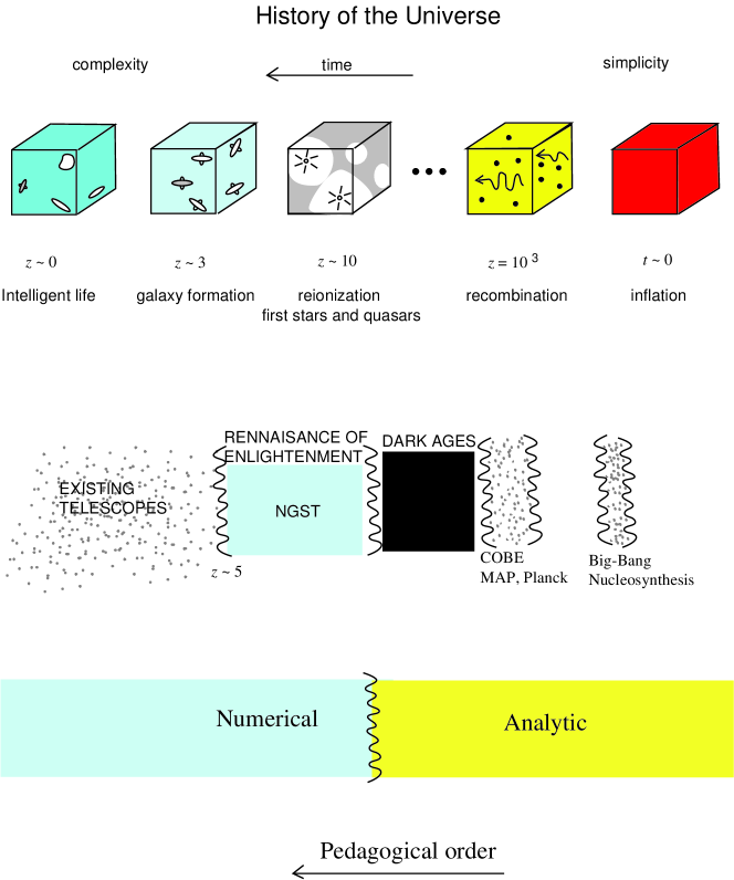
Figure 1: Milestones in the evolution of the universe from simplicity to complexity. The “end of the dark ages” bridges between the recombination epoch probed by microwave anisotropy experiments ($z\sim 10^{3}$) and the horizon of current observations ($z\sim 5$–6).

For these reasons, advances in technology are likely to make the high redshift universe an important frontier of cosmology over the coming decade. This effort will involve large (30 meter) ground-based telescopes and will culminate in the launch of the successor to the Hubble Space Telescope,  called Next Generation Space Telescope (NGST ). NGST,  planned for launch in 2009, will image the first sources of light that formed in the universe. With its exceptional sub-nJy ($1~{}{\rm nJy}=10^{-32}{\rm erg~{}cm^{-2}~{}s^{-1}~{}Hz^{-1}}$) sensitivity in the 1–3.5$\mu$m infrared regime, NGST  is ideally suited for probing optical-UV emission from sources at redshifts $\mathrel{\hbox{\hbox to0.0pt{\hbox{\lower 4.0pt\hbox{$\sim$}}\hss}\hbox{$>$}}}10$, just when popular Cold Dark Matter models for structure formation predict the first baryonic objects to have collapsed.

The study of the the formation of the first generation of sources at early cosmic times (high redshifts) holds the key to constraining the power-spectrum of density fluctuations on small scales. Previous research in cosmology has been dominated by studies of Large Scale Structure (LSS); future studies are likely to focus on Small Scale Structure (SSS).

The first sources are a direct consequence of the growth of linear density fluctuations. As such, they emerge from a well-defined set of initial conditions and the physics of their formation can be followed precisely by computer simulation. The cosmic initial conditions for the formation of the first generation of stars are much simpler than those responsible for star formation in the Galactic interstellar medium at present. The cosmic conditions are fully specified by the primordial power spectrum of Gaussian density fluctuations, the mean density of dark matter, the initial temperature and density of the cosmic gas, the primordial composition according to Big-Bang nucleosynthesis, and the lack of dynamically-significant magnetic fields. The chemistry is much simpler in the absence of metals and the gas dynamics is much simpler in the absence of dynamically-important magnetic fields.

The initial mass function of the first stars and black holes is therefore determined by a simple set of initial conditions (although subsequent generations of stars are affected by feedback from photoionization heating and metal enrichment). While the early evolution of the seed density fluctuations can be fully described analytically, the collapse and fragmentation of nonlinear structure must be simulated numerically. The first baryonic objects connect the simple initial state of the universe to its complex current state, and their study with hydrodynamic simulations (e.g., Abel, Bryan, & Norman 2000; Bromm, Coppi, & Larson 1999) and with future telescopes such as NGST  offers the key to advancing our knowledge on the formation physics of stars and massive black holes.

The first light from stars and quasars ended the “dark ages” of the universe and initiated a “renaissance of enlightenment” in the otherwise fading glow of the microwave background (see Figure 1). It is easy to see why the mere conversion of trace amounts of gas into stars or black holes at this early epoch could have had a dramatic effect on the ionization state and temperature of the rest of the gas in the universe. Nuclear fusion releases $\sim 7\times 10^{6}$ eV per hydrogen atom, and thin-disk accretion onto a Schwarzschild black hole releases ten times more energy; however, the ionization of hydrogen requires only 13.6 eV. It is therefore sufficient to convert a small fraction, $\sim 10^{-5}$ of the total baryonic mass into stars or black holes in order to ionize the rest of the universe. (The actual required fraction is higher by at least an order of magnitude [Bromm, Kudritzky, & Loeb 2000] because only some of the emitted photons are above the ionization threshold of 13.6 eV and because each hydrogen atom recombines more than once at redshifts $z\mathrel{\hbox{\hbox to0.0pt{\hbox{\lower 4.0pt\hbox{$\sim$}}\hss}\hbox{$>$}}}7$). Recent calculations of structure formation in popular CDM cosmologies imply that the universe was ionized at $z\sim 7$–12 (Haiman & Loeb 1998, 1999b,c; Gnedin & Ostriker 1998; Chiu & Ostriker 2000; Gnedin 2000a). Current observations are at the threshold of probing this epoch of reionization, given the fact that galaxies and quasars at redshifts $\sim 6$ are being discovered (Fan et al. 2000; Stern et al. 2000). One of these sources is a bright quasar at $z=5.8$ whose spectrum is shown in Figure 2. The plot indicates that there is transmitted flux shortward of the Ly$\alpha$ wavelength at the quasar redshift. However, Gunn & Peterson (1965) showed that even a tiny neutral hydrogen fraction in the intergalactic medium would produce a large optical depth at these wavelengths. Indeed, modeling of the transmitted flux (Fan et al. 2000) implies an optical depth $\tau<0.5$ or a neutral fraction $x_{\rm H\,I}\mathrel{\hbox{\hbox to0.0pt{\hbox{\lower 4.0pt\hbox{$\sim$}}\hss}\hbox{$<$}}}10^{-6}$, i.e., the universe is fully ionized at $z=5.8$! One of the important challenges of future observations will be to identify when and how the intergalactic medium was ionized. Theoretical calculations (see §2.3) imply that such observations are just around the corner.

Figure 2: Optical spectrum of the highest-redshift known quasar at $z=5.8$, discovered by the Sloan Digital Sky Survey (Fan et al.  2000).

Figure 3 shows schematically the various stages in a theoretical scenario for the history of hydrogen reionization in the intergalactic medium. The first gaseous clouds collapse at redshifts $\sim 20$–$30$ and fragment into stars due to molecular hydrogen (H₂) cooling. However, H₂ is fragile and can be easily dissociated by a small flux of UV radiation (Stecher & Williams 1967; Haiman, Rees, & Loeb 1997). Hence the bulk of the radiation that ionized the universe is emitted from galaxies with a virial temperature $\mathrel{\hbox{\hbox to0.0pt{\hbox{\lower 4.0pt\hbox{$\sim$}}\hss}\hbox{$>$}}}10^{4}$ K, where atomic cooling is effective and allows the gas to fragment (see Haiman, Abel, & Rees 1999 for an alternative scenario).

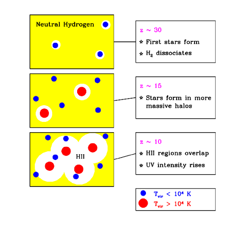
Figure 3: Stages in the reionization of hydrogen in the intergalactic medium.

Since recent observations confine the standard set of cosmological parameters to a relatively narrow range, we assume a $\Lambda$CDM cosmology with a particular standard set of parameters in the quantitative results in this review. For the contributions to the energy density, we assume ratios relative to the critical density of ${\Omega_{m}}=0.3$, ${\Omega_{\Lambda}}=0.7$, and $\Omega_{b}=0.045$, for matter, vacuum (cosmological constant), and baryons, respectively. We also assume a Hubble constant $H_{0}=70\mbox{ km s}^{-1}\mbox{Mpc}^{-1}$, and a primordial scale invariant ($n=1$) power spectrum with $\sigma_{8}=0.9$, where $\sigma_{8}$ is the root-mean-square amplitude of mass fluctuations in spheres of radius $8\ h^{-1}$ Mpc. These parameter values are based primarily on the following observational results: CMB temperature anisotropy measurements on large scales (Bennett et al. 1996) and on the scale of $\sim 1^{\circ}$ (Lange et al. 2000; Balbi et al. 2000); the abundance of galaxy clusters locally (Viana & Liddle 1999; Pen 1998; Eke, Cole, & Frenk 1996) and as a function of redshift (Bahcall & Fan 1998; Eke, Cole, Frenk, & Henry 1998); the baryon density inferred from big bang nucleosynthesis (see the review by Tytler et al. 2000); distance measurements used to derive the Hubble constant (Mould et al. 2000; Jha et al. 1999; Tonry et al. 1997); and indications of cosmic acceleration from distances based on type Ia supernovae (Perlmutter et al. 1999; Riess et al. 1998).

This review summarizes recent theoretical advances in understanding the physics of the first generation of cosmic structures. Although the literature on this subject extends all the way back to the sixtees (Saslaw & Zipoy 1967, Peebles & Dicke 1968, Hirasawa 1969, Matsuda et al. 1969, Hutchins 1976, Silk 1983, Palla et al. 1983, Lepp & Shull 1984, Couchman 1985, Couchman & Rees 1986, Lahav 1986), this review focuses on the progress made over the past decade in the modern context of CDM cosmologies.

2 RADIATIVE FEEDBACK FROM THE FIRST SOURCES OF LIGHT

2.1 Escape of Ionizing Radiation from Galaxies

The intergalactic ionizing radiation field, a key ingredient in the development of reionization, is determined by the amount of ionizing radiation escaping from the host galaxies of stars and quasars. The value of the escape fraction as a function of redshift and galaxy mass remains a major uncertainty in all current studies, and could affect the cumulative radiation intensity by orders of magnitude at any given redshift. Gas within halos is far denser than the typical density of the IGM, and in general each halo is itself embedded within an overdense region, so the transfer of the ionizing radiation must be followed in the densest regions in the universe. Reionization simulations are limited in resolution and often treat the sources of ionizing radiation and their immediate surroundings as unresolved point sources within the large-scale intergalactic medium (see, e.g., Gnedin 2000a).

The escape of ionizing radiation ($h\nu>13.6$eV, $\lambda<912$ Å) from the disks of present-day galaxies has been studied in recent years in the context of explaining the extensive diffuse ionized gas layers observed above the disk in the Milky Way (Reynolds et al. 1995) and other galaxies (e.g., Rand 1996; Hoopes, Walterbos, & Rand 1999). Theoretical models predict that of order 3–14% of the ionizing luminosity from O and B stars escapes the Milky Way disk (Dove & Shull 1994; Dove, Shull, & Ferrara 2000). A similar escape fraction of $f_{\rm esc}=6$% was determined by Bland-Hawthorn & Maloney (1999) based on H$\alpha$ measurements of the Magellanic Stream. From Hopkins Ultraviolet Telescope observations of four nearby starburst galaxies (Leitherer et al. 1995; Hurwitz, Jelinsky, & Dixon 1997), the escape fraction was estimated to be in the range 3%$<f_{\rm esc}<57$%. If similar escape fractions characterize high redshift galaxies, then stars could have provided a major fraction of the background radiation that reionized the IGM (e.g., Madau & Shull 1996; Madau 1999). However, the escape fraction from high-redshift galaxies, which formed when the universe was much denser ($\rho\propto(1+z)^{3}$), may be significantly lower than that predicted by models ment to describe present-day galaxies. Current reionization calculations assume that galaxies are isotropic point sources of ionizing radiation and adopt escape fractions in the range $5\%<f_{\rm esc}<60\%$ (see, e.g., Gnedin 2000a, Miralda-Escudé et al. 1999).

Clumping is known to have a significant effect on the penetration and escape of radiation from an inhomogeneous medium (e.g., Boissé 1990; Witt & Gordon 1996, 2000; Neufeld 1991; Haiman & Spaans 1999; Bianchi et al. 2000). The inclusion of clumpiness introduces several unknown parameters into the calculation, such as the number and overdensity of the clumps, and the spatial correlation between the clumps and the ionizing sources. An additional complication may arise from hydrodynamic feedback, whereby part of the gas mass is expelled from the disk by stellar winds and supernovae [see §7 of Barkana & Loeb (2000c) for a review of this topic].

Wood & Loeb (2000) used a three-dimensional radiation transfer code to calculate the steady-state escape fraction of ionizing photons from disk galaxies as a function of redshift and galaxy mass. The gaseous disks were assumed to be isothermal, with a sound speed $c_{s}\sim 10~{}{\rm km~{}s^{-1}}$, and radially exponential. For stellar sources, the predicted increase in the disk density with redshift resulted in a strong decline of the escape fraction with increasing redshift. The situation is different for a central quasar. Due to its higher luminosity and central location, the quasar tends to produce an ionization channel in the surrounding disk through which much of its ionizing radiation escapes from the host. In a steady state, only recombinations in this ionization channel must be balanced by ionizations, while for stars there are many ionization channels produced by individual star-forming regions and the total recombination rate in these channels is very high. Escape fractions $\mathrel{\hbox{\hbox to0.0pt{\hbox{\lower 4.0pt\hbox{$\sim$}}\hss}\hbox{$>$}}}10\%$ were achieved for stars at $z\sim 10$ only if $\sim 90\%$ of the gas was expelled from the disks or if dense clumps removed the gas from the vast majority ($\mathrel{\hbox{\hbox to0.0pt{\hbox{\lower 4.0pt\hbox{$\sim$}}\hss}\hbox{$>$}}}80\%$) of the disk volume (see Figure 4). This analysis applies only to halos with virial temperatures $\mathrel{\hbox{\hbox to0.0pt{\hbox{\lower 4.0pt\hbox{$\sim$}}\hss}\hbox{$>$}}}10^{4}$ K. Ricotti & Shull (2000) reached similar conclusions but for a quasi-spherical configuration of stars and gas. They demonstrated that the escape fraction is substantially higher in low-mass halos with a virial temperature $\mathrel{\hbox{\hbox to0.0pt{\hbox{\lower 4.0pt\hbox{$\sim$}}\hss}\hbox{$<$}}}10^{4}$ K. However, the formation of stars in such halos depends on their uncertain ability to cool via the efficient production of molecular hydrogen (Haiman, Rees, & Loeb 1997; Haiman, Abel, & Rees 1999).

Figure 4: Escape fractions of stellar ionizing photons from a gaseous disk embedded within a $10^{10}M_{\odot}$ halo which have formed at $z=10$ (from Wood & Loeb 2000). The curves show three different cases of clumpiness within the disk. The volume filling factor refers to either the ionizing emissivity, the gas clumps, or both, depending on the case. The escape fraction is substantial ($\mathrel{\hbox{\hbox to0.0pt{\hbox{\lower 4.0pt\hbox{$\sim$}}\hss}\hbox{$>$}}}1\%$) only if the gas distribution is highly clumped.

The main uncertainty in the above predictions involves the distribution of the gas inside the host galaxy, as the gas is exposed to the radiation released by stars and the mechanical energy deposited by supernovae. Given the fundamental role played by the escape fraction, it is desirable to calibrate its value observationally. Recently, Steidel, Pettini, & Adelberger (2000) reported a preliminary detection of significant Lyman continuum flux in the composite spectrum of 29 Lyman break galaxies (LBG) with redshifts in the range $z=3.40\pm 0.09$. After correcting for intergalactic absorption, Steidel et al. (2000) inferred a ratio between the emergent flux density at 1500Å  and 900Å  (rest frame) of $4.6\pm 1.0$. Taking into account the fact that the stellar spectrum should already have an intrinsic Lyman discontinuity of a factor of $\sim 3$–5, but that only $\sim 15$–$20\%$ of the 1500Å  photons escape from typical LBGs without being absorbed by dust (Pettini et al. 1998a; Adelberger & Steidel 2000), the inferred 900Å  escape fraction is $f_{\rm esc}\sim 10$–$20\%$. Although the galaxies in this sample were drawn from the bluest quartile of the LBG spectral energy distributions, the measurement implies that this quartile may itself dominate the hydrogen-ionizing background relative to quasars at $z\sim 3$.

2.2 Propagation of Ionization Fronts in the IGM

The radiation output from the first stars ionizes hydrogen in a growing volume, eventually encompassing almost the entire IGM within a single H II bubble. In the early stages of this process, each galaxy produces a distinct H II region, and only when the overall H II filling factor becomes significant do neighboring bubbles begin to overlap in large numbers, ushering in the “overlap phase” of reionization. Thus, the first goal of a model of reionization is to describe the initial stage, when each source produces an isolated expanding H II region.

We assume a spherical ionized volume which is separated from the surrounding neutral gas by a sharp ionization front. Indeed, in the case of a stellar ionizing spectrum, most ionizing photons are just above the hydrogen ionization threshold of 13.6 eV, where the absorption cross-section is high and a very thin layer of neutral hydrogen is sufficient to absorb all the ionizing photons. On the other hand, an ionizing source such as a quasar produces significant numbers of higher energy photons and results in a thicker transition region.

In the absence of recombinations, each hydrogen atom in the IGM would only have to be ionized once. However, the increased density of the IGM at high redshift implies that recombinations cannot be neglected, since the recombination rate depends on the square of the gas density. Thus, if the IGM is not uniform, but instead the gas which is being ionized is mostly distributed in high-density clumps, then the recombination rate is very high. This is often dealt with by introducing a volume-averaged clumping factor $C$ (in general time-dependent), defined by

$$C=\left<n_{H}^{2}\right>/\bar{n}_{H}^{2}\ .$$ (1)

If the ionized volume is large compared to the typical scale of clumping, so that many clumps are averaged over, then the solution for the comoving volume $V(t)$ (generalized from Shapiro & Giroux 1987; see Barkana & Loeb 2000c) around a source which turns on at $t=t_{i}$ is

$$V(t)=\int_{t_{i}}^{t}\frac{1}{\bar{n}_{H}^{0}}\frac{d\,N_{\gamma}}{dt^{\prime}}\,e^{F(t^{\prime},t)}dt^{\prime}\ ,$$ (2)

where

$$F(t^{\prime},t)=-\alpha_{B}\bar{n}_{H}^{0}\int_{t^{\prime}}^{t}\frac{C(t^{\prime\prime})}{a^{3}(t^{\prime\prime})}\,dt^{\prime\prime}\ .$$ (3)

In these expressions, $dN_{\gamma}/dt$ is the rate at which the source produces ionizing photons, $\bar{n}_{H}^{0}$ is the present number density of hydrogen, $a$ is the scale factor, and $\alpha_{B}$ is the case B recombination coefficient for hydrogen at $T=10^{4}$ K.

The size of the resulting H II region depends on the halo which produces it. Consider a halo of total mass $M$ and baryon fraction $\Omega_{b}/{\Omega_{m}}$. To derive a rough estimate, we assume that baryons are incorporated into stars with an efficiency of $f_{\rm star}=10\%$, and that the escape fraction for the resulting ionizing radiation is also $f_{\rm esc}=10\%$. If the stellar IMF is similar to the one measured locally (Scalo 1998), then $N_{\gamma}\approx 4000$ ionizing photons are produced per baryon in stars (for a metallicity equal to $1/20$ of the solar value). We define a parameter which gives the overall number of ionizations per baryon,

$$N_{\rm ion}\equiv N_{\gamma}\,f_{\rm star}\,f_{\rm esc}\ .$$ (4)

If we neglect recombinations then we obtain the maximum comoving radius of the region which the halo of mass $M$ can ionize,

$$r_{\rm max}=\left(\frac{3}{4\pi}\,\frac{N_{\gamma}}{\bar{n}_{H}^{0}}\right)^{1/3}=\left(\frac{3}{4\pi}\,\frac{N_{\rm ion}}{\bar{n}_{H}^{0}}\,\frac{\Omega_{b}}{{\Omega_{m}}}\,\frac{M}{m_{p}}\right)^{1/3}=680\,{\rm kpc}\left(\frac{N_{\rm ion}}{40}\,\frac{M}{10^{8}M_{\hbox{$\odot$}}}\right)^{1/3}\ ,$$ (5)

for our standard choice of cosmological parameters: ${\Omega_{m}}=0.3$, ${\Omega_{\Lambda}}=0.7$, and $\Omega_{b}=0.045$. The actual radius never reaches this size if the recombination time is shorter than the lifetime of the ionizing source.

In Figure 5 we show the time evolution of the volume ionized by such a source which undergoes an instantaneous starburst with the Scalo (1998) IMF. The volume is shown in units of the maximum volume $V_{\rm max}$ which corresponds to $r_{\rm max}$ in equation (5). We consider a source turning on at $z=10$ (solid curves) or $z=15$ (dashed curves), with three cases for each: no recombinations, $C=1$, and $C=10$, in order from top to bottom (Note that the result is independent of redshift in the case of no recombinations; also, in every case we assume a time-independent $C$). When recombinations are included, the volume rises and reaches close to $V_{\rm max}$ before dropping after the source turns off. At large $t$ recombinations stop due to the dropping density, and the volume approaches a constant value (although $V\ll V_{\rm max}$ at large $t$ if $C=10$).

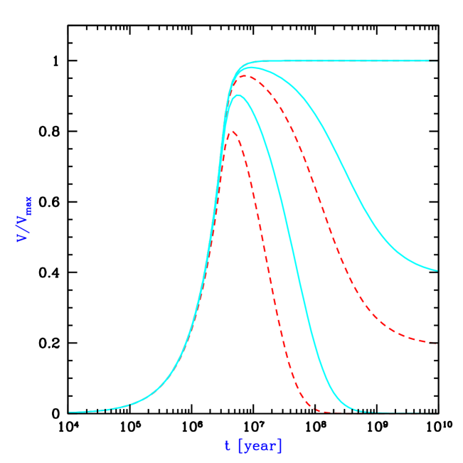
Figure 5: Expanding H II region around an isolated ionizing source. The comoving ionized volume $V$ is expressed in units of the maximum possible volume, $V_{\rm max}=4\pi r_{\rm max}^{3}/3$ [with $r_{\rm max}$ given in equation (5)], and the time is measured after an instantaneous starburst which is characterized by a Scalo (1998) IMF. We consider a source turning on at $z=10$ (solid curves) or $z=15$ (dashed curves), with three cases for each: no recombinations, $C=1$, and $C=10$, in order from top to bottom. The no-recombination curve is identical for the different source redshifts.

We obtain a similar result for the size of the H II region around a galaxy if we consider a mini-quasar rather than stars. For the typical quasar spectrum (Elvis et al. 1994), if we assume a radiative efficiency of $\sim 6\%$ then roughly 11,000 ionizing photons are produced per baryon incorporated into the black hole (Haiman, personal communication). The efficiency of incorporating the baryons in a galaxy into a central black hole is low ($\mathrel{\hbox{\hbox to0.0pt{\hbox{\lower 4.0pt\hbox{$\sim$}}\hss}\hbox{$<$}}}0.6\%$ in the local universe, e.g. Magorrian et al. 1998; see also §3.3), but the escape fraction for quasars is likely to be close to unity, i.e., an order of magnitude higher than for stars (see §2.1). Thus, for every baryon in galaxies, up to $\sim 65$ ionizing photons may be produced by a central black hole and $\sim 40$ by stars, although both of these numbers for $N_{\rm ion}$ are highly uncertain. These numbers suggest that in either case the typical size of H II regions before reionization may be $\mathrel{\hbox{\hbox to0.0pt{\hbox{\lower 4.0pt\hbox{$\sim$}}\hss}\hbox{$<$}}}1$ Mpc or $\sim 10$ Mpc, depending on whether $10^{8}M_{\hbox{$\odot$}}$ halos or $10^{12}M_{\hbox{$\odot$}}$ halos dominate.

2.3 Reionization of Hydrogen in the IGM

In this section we summarize recent progress, both analytic and numerical, made toward elucidating the basic physics of reionization and the way in which the characteristics of reionization depend on the nature of the ionizing sources and on other input parameters of cosmological models.

The process of the reionization of hydrogen involves several distinct stages. The initial, “pre-overlap” stage (using the terminology of Gnedin 2000a) consists of individual ionizing sources turning on and ionizing their surroundings. The first galaxies form in the most massive halos at high redshift, and these halos are biased and are preferentially located in the highest-density regions. Thus the ionizing photons which escape from the galaxy itself (see §2.1) must then make their way through the surrounding high-density regions, which are characterized by a high recombination rate. Once they emerge, the ionization fronts propagate more easily into the low-density voids, leaving behind pockets of neutral, high-density gas. During this period the IGM is a two-phase medium characterized by highly ionized regions separated from neutral regions by ionization fronts. Furthermore, the ionizing intensity is very inhomogeneous even within the ionized regions, with the intensity determined by the distance from the nearest source and by the ionizing luminosity of this source.

The central, relatively rapid “overlap” phase of reionization begins when neighboring H II regions begin to overlap. Whenever two ionized bubbles are joined, each point inside their common boundary becomes exposed to ionizing photons from both sources. Therefore, the ionizing intensity inside H II regions rises rapidly, allowing those regions to expand into high-density gas which had previously recombined fast enough to remain neutral when the ionizing intensity had been low. Since each bubble coalescence accelerates the process of reionization, the overlap phase has the character of a phase transition and is expected to occur rapidly, over less than a Hubble time at the overlap redshift. By the end of this stage most regions in the IGM are able to see several unobscured sources, and therefore the ionizing intensity is much higher than before overlap and it is also much more homogeneous. An additional ingredient in the rapid overlap phase results from the fact that hierarchical structure formation models predict a galaxy formation rate that rises rapidly with time at the relevant redshift range. This process leads to a state in which the low-density IGM has been highly ionized and ionizing radiation reaches everywhere except for gas located inside self-shielded, high-density clouds. This marks the end of the overlap phase, and this important landmark is most often referred to as the ’moment of reionization’.

Some neutral gas does, however, remain in high-density structures which correspond to Lyman Limit systems and damped Ly$\alpha$ systems seen in absorption at lower redshifts. The high-density regions are gradually ionized as galaxy formation proceeds, and the mean ionizing intensity also grows with time. The ionizing intensity continues to grow and to become more uniform as an increasing number of ionizing sources is visible to every point in the IGM. This “post-overlap” phase continues indefinitely, since collapsed objects retain neutral gas even in the present universe. The IGM does, however, reach another milestone at $z\sim 1.6$, the breakthrough redshift (Madau, Haardt, & Rees 1999). Below this redshift, all ionizing sources are visible to each other, while above this redshift absorption by the Ly$\alpha$ forest clouds implies that only sources in a small redshift range are visible to a typical point in the IGM.

Semi-analytic models of the pre-overlap stage focus on the evolution of the H II filling factor $Q_{\rm H\ II}$, i.e., the fraction of the volume of the universe which is filled by H II regions. The model of individual H II regions presented in the previous section can be used to understand the development of the total filling factor. The overall production of ionizing photons depends on the collapse fraction $F_{\rm col}$, the fraction of all the baryons in the universe which are in galaxies, i.e., the fraction of gas which settles into halos and cools efficiently inside them. For simplicity, we assume instantaneous production of photons, i.e., that the timescale for the formation and evolution of the massive stars in a galaxy is short compared to the Hubble time at the formation redshift of the galaxy. We also neglect other complications (such as inhomogeneous clumping and source clustering) which are discussed below. Under these assumptions, we can convert equation (2), which describes individual H II regions, to an equation which statistically describes the transition from a neutral universe to a fully ionized one (see Barkana & Loeb 2000c; also Madau et al. 1999 and Haiman & Loeb 1997):

$$Q_{\rm H\ II}(t)=\int_{0}^{t}\frac{N_{\rm ion}}{0.76}\frac{dF_{\rm col}}{dt^{\prime}}\,e^{F(t^{\prime},t)}dt^{\prime}\ ,$$ (6)

where $F(t^{\prime},t)$ is determined by equation (3).

A simple estimate of the collapse fraction at high redshift is the mass fraction [given, e.g., by the model of Press-Schechter (1974)] in halos above the cooling threshold, which is the minimum mass of halos in which gas can cool efficiently. Assuming that only atomic cooling is effective during the redshift range of reionization (Haiman, Rees, & Loeb 1997), the minimum mass corresponds roughly to a halo of virial temperature $T_{\rm vir}=10^{4}$ K, which corresponds to a total halo mass of $\sim 8\times 10^{7}M_{\hbox{$\odot$}}$ at $z=10$. With this prescription we derive (for $N_{\rm ion}=40$) the reionization history shown in Figure 6 for the case of a constant clumping factor $C$. The solid curves show $Q_{\rm H\ II}$ as a function of redshift for a clumping factor $C=0$ (no recombinations), $C=1$, $C=10$, and $C=30$, in order from left to right. Note that if $C\sim 1$ then recombinations are unimportant, but if $C\mathrel{\hbox{\hbox to0.0pt{\hbox{\lower 4.0pt\hbox{$\sim$}}\hss}\hbox{$>$}}}10$ then recombinations significantly delay the reionization redshift (for a fixed star-formation history). The dashed curve shows the collapse fraction $F_{\rm col}$ in this model. For comparison, the vertical dotted line shows the $z=5.8$ observational lower limit (Fan et al. 2000) on the reionization redshift.

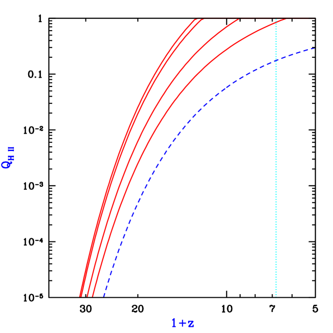
Figure 6: Semi-analytic calculation of the reionization of the IGM (for $N_{\rm ion}=40$), showing the redshift evolution of the filling factor $Q_{\rm H\ II}$. Solid curves show $Q_{\rm H\ II}$ for a clumping factor $C=0$ (no recombinations), $C=1$, $C=10$, and $C=30$, in order from left to right. The dashed curve shows the collapse fraction $F_{\rm col}$, and the vertical dotted line shows the $z=5.8$ observational lower limit (Fan et al. 2000) on the reionization redshift.

Clearly, star-forming galaxies in CDM hierarchical models are capable of ionizing the universe at $z\sim 6$–15 with reasonable parameter choices. This has been shown by a number of theoretical, semi-analytic calculations (Fukugita & Kawasaki 1994; Shapiro, Giroux, & Babul 1994; Haiman & Loeb 1997; Valageas & Silk 1999; Chiu & Ostriker 2000; Ciardi et al. 2000) as well as numerical simulations (Cen & Ostriker 1993; Gnedin & Ostriker 1997; Gnedin 2000a). Similarly, if a small fraction ($\mathrel{\hbox{\hbox to0.0pt{\hbox{\lower 4.0pt\hbox{$\sim$}}\hss}\hbox{$<$}}}1\%$) of the gas in each galaxy accretes onto a central black hole, then the resulting mini-quasars are also able to reionize the universe, as has also been shown using semi-analytic models (Fukugita & Kawasaki 1994; Haiman & Loeb 1998; Valageas & Silk 1999). Note that the prescription whereby a constant fraction of the galactic mass accretes onto a central black hole is based on local observations (see §3.3) which indicate that $z=0$ galaxies harbor central black holes of mass equal to $\sim 0.2$–$0.6\%$ of their bulge mass. Although the bulge constitutes only a fraction of the total baryonic mass of each galaxy, the higher gas-to-stellar mass ratio in high redshift galaxies, as well as their high merger rates compared to their low redshift counterparts, suggest that a fraction of a percent of the total gas mass in high-redshift galaxies may have contributed to the formation of quasar black holes.

Although many models yield a reionization redshift around 7–12, the exact value depends on a number of uncertain parameters affecting both the sources and the overall recombination rate. The source parameters include the formation efficiency of stars and quasars and the escape fraction of ionizing photons produced by these sources (§2.1). The formation efficiency of low mass galaxies may also be reduced by feedback from galactic outflows [e.g., Dekel & Silk 1986; Mac Low & Ferrara 1999; see §7 of Barkana & Loeb (2000c) for a review of this topic]. Even when the clumping is inhomogeneous, the treatment in equation (6) is generally valid if $C$ is defined as in equation (1), where we take a global volume average of the square of the density inside ionized regions (since neutral regions do not contribute to the recombination rate). The resulting mean clumping factor depends on the density and clustering of sources, and on the distribution and topology of density fluctuations in the IGM. Furthermore, the source halos should tend to form in overdense regions, and the clumping factor is affected by this cross-correlation between the sources and the IGM density.

Miralda-Escudé, Haehnelt, & Rees (2000) presented a simple model for the distribution of density fluctuations, and more generally they discussed the implications of inhomogeneous clumping during reionization. They noted that as ionized regions grow, they more easily extend into low-density regions, and they tend to leave behind high-density concentrations, with these neutral islands being ionized only at a later stage. They therefore argued that, since at high-redshift the collapse fraction is low, most of the high-density regions, which would dominate the clumping factor if they were ionized, will in fact remain neutral and occupy only a tiny fraction of the total volume. Thus, the development of reionization through the end of the overlap phase should occur almost exclusively in the low-density IGM, and the effective clumping factor during this time should be $\sim 1$, making recombinations relatively unimportant (see Figure 6). Only in the post-reionization phase, Miralda-Escudé et al. (2000) argued, do the high density clouds and filaments become gradually ionized as the mean ionizing intensity further increases.

The complexity of the process of reionization is illustrated by the recent numerical simulation by Gnedin (2000a) of stellar reionization (in $\Lambda$CDM with ${\Omega_{m}}=0.3$). This simulation uses a formulation of radiative transfer which relies on several rough approximations; although it does not include the effect of shadowing behind optically-thick clumps, it does include for each point in the IGM the effects of an estimated local optical depth around that point, plus a local optical depth around each ionizing source. This simulation helps to understand the advantages of the various theoretical approaches, while pointing to the complications which are not included in the simple models. Figures 7 and 8, taken from Figure 3 in Gnedin (2000a), show the state of the simulated universe just before and just after the overlap phase, respectively. They show a thin (15 $h^{-1}$ comoving kpc) slice through the box, which is 4 $h^{-1}$ Mpc on a side, achieves a spatial resolution of $1h^{-1}$ kpc, and uses $128^{3}$ each of dark matter particles and baryonic particles (with each baryonic particle having a mass of $5\times 10^{5}M_{\hbox{$\odot$}}$). The figures show the redshift evolution of the mean ionizing intensity $J_{21}$ (upper right panel), and visually the logarithm of the neutral hydrogen fraction (upper left panel), the gas density (lower left panel), and the gas temperature (lower right panel). Note the obvious features resulting from the periodic boundary conditions assumed in the simulation. Also note that the intensity $J_{21}$ is defined as the intensity at the Lyman limit, expressed in units of $10^{-21}\,\mbox{ erg cm}^{-2}\mbox{ s}^{-1}\mbox{ sr}^{-1}\mbox{Hz}^{-1}$. For a given source emission, the intensity inside H II regions depends on absorption and radiative transfer through the IGM (e.g., Haardt & Madau 1996; Abel & Haehnelt 1999)

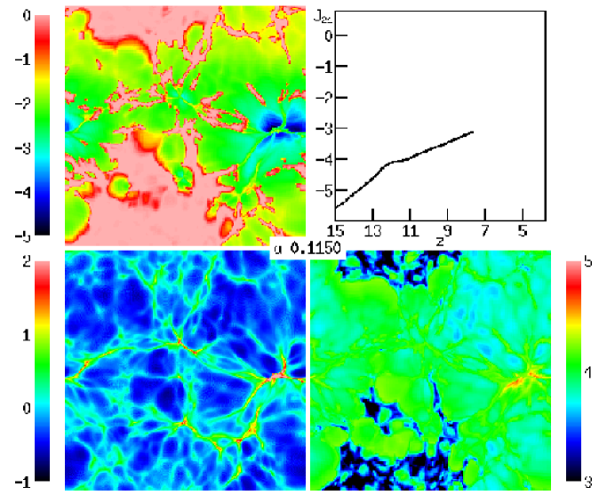
Figure 7: Visualization at $z=7.7$ of a numerical simulation of reionization, adopted from Figure 3c of Gnedin (2000a). The panels display the logarithm of the neutral hydrogen fraction (upper left), the gas density (lower left), and the gas temperature (lower right). Also shown is the redshift evolution of the logarithm of the mean ionizing intensity (upper right). Note the periodic boundary conditions.

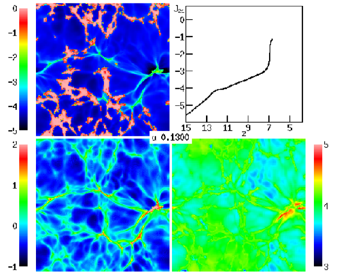
Figure 8: Visualization at $z=6.7$ of a numerical simulation of reionization, adopted from Figure 3e of Gnedin (2000a). The panels display the logarithm of the neutral hydrogen fraction (upper left), the gas density (lower left), and the gas temperature (lower right). Also shown is the redshift evolution of the logarithm of the mean ionizing intensity (upper right). Note the periodic boundary conditions.

Figure 7 shows the two-phase IGM at $z=7.7$, with ionized bubbles emanating from one main concentration of sources (located at the right edge of the image, vertically near the center; note the periodic boundary conditions). The bubbles are shown expanding into low density regions and beginning to overlap at the center of the image. The topology of ionized regions is clearly complex: While the ionized regions are analogous to islands in an ocean of neutral hydrogen, the islands themselves contain small lakes of dense neutral gas. One aspect which has not been included in theoretical models of clumping is clear from the figure. The sources themselves are located in the highest density regions (these being the sites where the earliest galaxies form) and must therefore ionize the gas in their immediate vicinity before the radiation can escape into the low density IGM. For this reason, the effective clumping factor is of order 100 in the simulation and also, by the overlap redshift, roughly ten ionizing photons have been produced per baryon. Figure 8 shows that by $z=6.7$ the low density regions have all become highly ionized along with a rapid increase in the ionizing intensity. The only neutral islands left are the highest density regions (compare the two panels on the left). However, we emphasize that the quantitative results of this simulation must be considered preliminary, since the effects of increased resolution and a more accurate treatment of radiative transfer are yet to be explored. Methods are being developed for incorporating a more complete treatment of radiative transfer into three dimensional cosmological simulations (e.g., Abel, Norman, & Madau 1999; Razoumov & Scott 1999).

Gnedin, Ferrara, & Zweibel (2000) investigated an additional effect of reionization. They showed that the Biermann battery in cosmological ionization fronts inevitably generates coherent magnetic fields of an amplitude $\sim 10^{-19}$ Gauss. These fields form as a result of the breakout of the ionization fronts from galaxies and their propagation through the H I filaments in the IGM. Although the fields are too small to directly affect galaxy formation, they could be the seeds for the magnetic fields observed in galaxies and X-ray clusters today.

If quasars contribute substantially to the ionizing intensity during reionization then several aspects of reionization are modified compared to the case of pure stellar reionization. First, the ionizing radiation emanates from a single, bright point-source inside each host galaxy, and can establish an escape route (H II funnel) more easily than in the case of stars which are smoothly distributed throughout the galaxy (§2.1). Second, the hard photons produced by a quasar penetrate deeper into the surrounding neutral gas, yielding a thicker ionization front. Finally, the quasar X-rays catalyze the formation of $H_{2}$ molecules and allow stars to keep forming in very small halos (Haiman, Abel, & Rees 1999).

Oh (2000) showed that star-forming regions may also produce significant X-rays at high redshift. The emission is due to inverse Compton scattering of CMB photons off relativistic electrons in the ejecta, as well as thermal emission by the hot supernova remnant. The spectrum expected from this process is even harder than for typical quasars, and the hard photons photoionize the IGM efficiently by repeated secondary ionizations. The radiation, characterized by roughly equal energy per logarithmic frequency interval, would produce a uniform ionizing intensity and lead to gradual ionization and heating of the entire IGM. Thus, if this source of emission is indeed effective at high redshift, it may have a crucial impact in changing the topology of reionization. Even if stars dominate the emission, the hardness of the ionizing spectrum depends on the initial mass function. At high redshift it may be biased toward massive, efficiently ionizing stars (e.g., Abel, Bryan, & Norman 2000; Bromm, Coppi, & Larson 1999), but this remains very much uncertain.

Madau et al. (1999) and Miralda-Escudé et al. (2000) have studied the possible ionizing sources which brought about reionization by extrapolating from the observed populations of galaxies and quasars to higher redshift. The general conclusion is that a high-redshift source population similar to the one observed at $z=3$–4 would produce roughly the needed ionizing intensity for reionization. A precise conclusion, however, remains elusive because of the same kinds of uncertainties as those found in the models based on CDM: The typical escape fraction, and the faint end of the luminosity function, are both not well determined even at $z=3$–4, and in addition the clumping factor at high redshift must be known in order to determine the importance of recombinations. Future direct observations of the source population at redshifts approaching reionization may help resolve some of these questions.

2.4 Helium Reionization

The sources that reionized hydrogen very likely caused the single reionization of helium from He I to He II. Neutral helium is ionized by photons of 24.6 eV or higher energy, and its recombination rate is roughly equal to that of hydrogen. On the other hand, the ionization threshold of He II is 54.4 eV, and fully ionized helium recombines $\mathrel{\hbox{\hbox to0.0pt{\hbox{\lower 4.0pt\hbox{$\sim$}}\hss}\hbox{$>$}}}5$ times faster than hydrogen. This means that for both quasars and galaxies, the reionization of He II should occur later than the reionization of hydrogen, even though the number of helium atoms is smaller than hydrogen by a factor of 13. The lower redshift of He II reionization makes it more accessible to observations and allows it to serve in some ways as an observational preview of hydrogen reionization.

The Ly$\alpha$ absorption by intergalactic He II (at wavelength $304$Å) has been observed in four quasars at redshifts $2.4<z<3.2$ (Jakobsen et al. 1994; Davidsen et al. 1996; Hogan et al. 1997; Reimers et al. 1997; Anderson et al. 1999; Heap et al. 2000). The results are consistent among the different quasars, and we illustrate them here with one particular spectrum. In figure 9, adopted from Figure 4 of Heap et al. (2000), we show a portion of the spectrum of the $z=3.286$ quasar $Q\ 0302-003$, obtained with the Space Telescope Imaging Spectrograph on-board the Hubble Space Telescope.  The observed spectrum (solid line) is compared to a simulated spectrum (gray shading) based on the H I Ly$\alpha$ forest observed in the same quasar. In deriving the simulated spectrum, Heap et al. assumed a ratio of He II to H I column densities of 100, and pure turbulent line broadening. The wavelength range shown in the figure corresponds to He II Ly$\alpha$ in the redshift range 2.8–3.3.

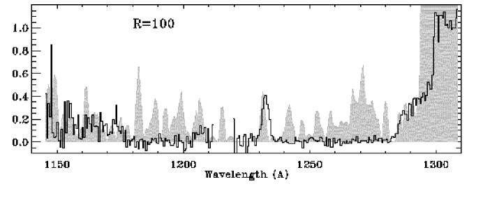
Figure 9: Ly$\alpha$ absorption by intergalactic He II. This spectrum of the $z=3.286$ quasar $Q\ 0302-003$, adopted from Figure 4 of Heap et al. (2000), was obtained using the Space Telescope Imaging Spectrograph. The observed spectrum (solid line) is compared to a simulated spectrum (gray shading) based on the H I Ly$\alpha$ forest observed in the same quasar. In deriving the simulated spectrum, Heap et al. assumed a ratio of He II to H I column densities of 100, and pure turbulent line broadening.

The observed flux shows a clear break short-ward of the quasar emission line at an observed $\lambda=1300$ Å. Relatively near the quasar, at $\lambda=$1285–1300Å, a shelf of relatively high transmission is likely evidence of the ’proximity effect’, in which the emission from the quasar itself creates a highly ionized local region with a reduced abundance of absorbing ions. In the region at $\lambda=$1240–1280 Å ($z=3.08$–3.21), on the other hand, the very low flux level implies an average optical depth of $\tau\sim 4.5$–5. Another large region with average $\tau\sim 4$, a region spanning $\sim 100$ comoving Mpc along the line of site, is evident at $\lambda=$1180–1210Å ($z=2.88$–2.98). The strong continuous absorption in these large regions, and the lack of correlation with the observed H I Ly$\alpha$ forest, is evidence for a He II Gunn-Peterson absorption trough due to the diffuse IGM. It also suggests a rather soft UV background with a significant stellar contribution, i.e., a background that ionizes the diffuse hydrogen much more thoroughly than He II. Significant emission is observed in between the two regions of constant high absorption. A small region around 1216Å is contaminated by geo-coronal Ly$\alpha$, but the emission at 1230–1235Å apparently corresponds to a real, distinct gap in the He II abundance, which could be caused by a local source photo-ionizing a region of radius $\sim 10$ comoving Mpc. The region at $\lambda=$1150–1175Å ($z=2.78$–2.86) shows a much higher overall transmission level than the regions at slightly higher redshift. Heap et al. measure an average $\tau=1.9$ in this region, and note that the significant correlation of the observed spectrum with the simulated one suggests that much of the absorption is due to a He II Ly$\alpha$ forest while the low-density IGM provides a relatively low opacity in this region. The authors conclude that the observed data suggest a sharp opacity break occurring between $z=3.0$ and 2.9, accompanied by a hardening of the UV ionizing background. However, even the relatively high opacity at $z\mathrel{\hbox{\hbox to0.0pt{\hbox{\lower 4.0pt\hbox{$\sim$}}\hss}\hbox{$>$}}}3$ only requires $\sim 0.1\%$ of helium atoms not to be fully ionized, in a region at the mean baryon density. Thus, the overlap phase of full helium reionization may have occurred significantly earlier, with the ionizing intensity already fairly uniform but still increasing with time at $z\sim 3$.

The properties of helium reionization have been investigated numerically by a number of authors. Zheng & Davidsen (1995) modeled the He II proximity effect, and a number of authors (Miralda-Escudé et al. 1996; Croft et al. 1997; Zhang et al. 1998) used numerical simulations to show that the observations generally agree with cold dark matter models. They also found that helium absorption particularly tests the properties of under-dense voids which produce much of the He II opacity but little opacity in H I. According to the semi-analytic model of inhomogeneous reionization of Miralda-Escudé, Haehnelt, & Rees (2000; see also §2.3), the total emissivity of observed quasars at redshift 3 suffices to completely reionize helium before $z=3$. They find that the observations at $z\sim 3$ can be reproduced if a population of low-luminosity sources, perhaps galaxies, has ionized the low-density IGM up to an overdensity of around 12, with luminous quasars creating the observed gaps of transmitted flux.

The conclusion that an evolution of the ionization state of helium has been observed is also strengthened by several indirect lines of evidence. Songaila & Cowie (1996) and Songaila (1998) found a rapid increase in the Si 4/C 4 ratio with decreasing redshift at $z=3$, for intermediate column density hydrogen Ly$\alpha$ absorption lines. They interpreted this evolution as a sudden hardening below $z=3$ of the spectrum of the ionizing background. Boksenberg et al. (1998) also found an increase in the Si 4/C 4 ratio, but their data implied a much more gradual increase from $z=3.8$ to $z=2.2$.

The full reionization of helium due to a hard ionizing spectrum should also heat the IGM to 20,000 K or higher, while the IGM can only reach $\sim$10,000 K during a reionization of hydrogen alone. This increase in temperature can serve as an observational probe of helium reionization, and it should also increase the suppression of dwarf galaxy formation (§2.6). The temperature of the IGM can be measured by searching for the smallest line-widths among hydrogen Ly$\alpha$ absorption lines (Schaye et al. 1999). In general, bulk velocity gradients contribute to the line width on top of thermal velocities, but a lower bound on the width is set by thermal broadening, and the narrowest lines can be used to measure the temperature. Several different measurements (Schaye et al. 2000; Ricotti et al. 2000; Bryan & Machacek 2000; McDonald et al. 2000) have found a nearly isothermal IGM at a temperature of $\sim$20,000 K at $z=3$, higher than expected in ionization equilibrium and suggestive of photo-heating due to ongoing reionization of helium. However, the measurement errors remain too large for a firm conclusion about the redshift evolution of the IGM temperature or its equation of state.

Clearly, the reionization of helium is already a rich phenomenological subject. Our knowledge will benefit from measurements of increasing accuracy, made toward many more lines of sight, and extended to higher redshift. New ways to probe helium will also be useful. For example, Miralda-Escudé (2000) has suggested that continuum He II absorption in soft X-rays can be used to determine the He II fraction along the line of sight, although the measurement requires an accurate subtraction of the Galactic contribution to the absorption, based on the Galactic H I column density as determined by 21 cm maps.

2.5 Photo-evaporation of Gaseous Halos After Reionization

The end of the reionization phase transition resulted in the emergence of an intense UV background that filled the universe and heated the IGM to temperatures of $\sim 1$–$2\times 10^{4}$K (see the previous section). After ionizing the rarefied IGM in the voids and filaments on large scales, the cosmic UV background penetrated the denser regions associated with the virialized gaseous halos of the first generation of objects. A major fraction of the collapsed gas had been incorporated by that time into halos with a virial temperature $\mathrel{\hbox{\hbox to0.0pt{\hbox{\lower 4.0pt\hbox{$\sim$}}\hss}\hbox{$<$}}}10^{4}$K, where the lack of atomic cooling prevented the formation of galactic disks and stars or quasars. Photoionization heating by the cosmic UV background could then evaporate much of this gas back into the IGM. The photo-evaporating halos, as well as those halos which did retain their gas, may have had a number of important consequences just after reionization as well as at lower redshifts.

In this section we focus on the process by which gas that had already settled into virialized halos by the time of reionization was evaporated back into the IGM due to the cosmic UV background. This process was investigated by Barkana & Loeb (1999) using semi-analytic methods and idealized numerical calculations. They first considered an isolated spherical, centrally-concentrated dark matter halo containing gas. Since most of the photo-evaporation occurs at the end of overlap, when the ionizing intensity builds up almost instantaneously, a sudden illumination by an external ionizing background may be assumed. Self-shielding of the gas implies that the halo interior sees a reduced intensity and a harder spectrum, since the outer gas layers preferentially block photons with energies just above the Lyman limit. It is useful to parameterize the external radiation field by a specific intensity per unit frequency, $\nu$,

$$J_{\nu}=10^{-21}\,J_{21}\,\left(\frac{\nu}{\nu_{L}}\right)^{-\alpha}\mbox{ erg cm}^{-2}\mbox{ s}^{-1}\mbox{ sr}^{-1}\mbox{Hz}^{-1}\ ,$$ (7)

where $\nu_{L}$ is the Lyman limit frequency, and $J_{21}$ is the intensity at $\nu_{L}$ expressed in units of $10^{-21}\,\mbox{ erg cm}^{-2}\mbox{ s}^{-1}\mbox{ sr}^{-1}\mbox{Hz}^{-1}$. The intensity is normalized to an expected post–reionization value of around unity for the ratio of ionizing photon density to the baryon density. Different power laws can be used to represent either quasar spectra ($\alpha\sim 1.8$) or stellar spectra ($\alpha\sim 5$).

Once the gas is heated throughout the halo, some fraction of it acquires a sufficiently high temperature that it becomes unbound. This gas expands due to the resulting pressure gradient and eventually evaporates back into the IGM. Figure 10 (adopted from Figure 3 of Barkana & Loeb 1999) shows the fraction of gas within the virial radius which becomes unbound after reionization, as a function of the total halo circular velocity, with halo masses at $z=8$ indicated at the top. The two pairs of curves correspond to spectral index $\alpha=5$ (solid) or $\alpha=1.8$ (dashed). In each pair, a calculation which assumes an optically-thin halo leads to the upper curve, but including radiative transfer and self-shielding modifies the result to the one shown by the lower curve. In each case self-shielding lowers the unbound fraction, but it mostly affects only a neutral core containing $\sim 30\%$ of the gas. Since high energy photons above the Lyman limit penetrate deep into the halo and heat the gas efficiently, a flattening of the spectral slope from $\alpha=5$ to $\alpha=1.8$ raises the unbound gas fraction. The characteristic circular velocity where most of the gas is lost is $\sim 10$–$15~{}{\rm km~{}s^{-1}}$ (roughly independent of redshift), but clearly the effect of photo-evaporation is gradual, going from total gas removal down to no effect over a range of a factor of $\sim 100$ in halo mass.

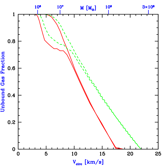
Figure 10: Effect of photo-evaporation on individual halos. The figure shows the unbound gas fraction (within the virial radius) versus total halo velocity dispersion or mass, adopted from Figure 3 of Barkana & Loeb (1999). The two pairs of curves correspond to spectral index $\alpha=5$ (solid) or $\alpha=1.8$ (dashed), in each case at $z=8$. In each pair, assuming an optically-thin halo leads to the upper curve, while the lower curve shows the result of including radiative transfer and self shielding.

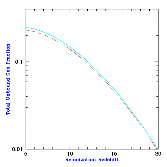
Figure 11: Effect of photo-evaporation on the overall halo population. The figure shows the total fraction of gas in the universe which evaporates from halos at reionization, versus the reionization redshift, adopted from Figure 7 of Barkana & Loeb (1999). The solid line assumes a spectral index $\alpha=1.8$, and the dotted line assumes $\alpha=5$.

Given the values of the unbound gas fraction in halos of different masses, the mass function of Press & Schechter (1974) can be used to calculate the total fraction of the IGM which goes through the process of accreting onto a halo and then being recycled into the IGM at reionization. The low-mass cutoff in this sum over halos is given by the lowest mass halo in which gas has assembled by the reionization redshift. This mass can be estimated by the linear Jeans mass (e.g., §6 of Peebles 1993), which is $\sim 10^{4}M_{\odot}$ at $z=15$. The Jeans mass is sufficiently accurate since at $z\sim 10$–20 it agrees well with the values found in the numerical spherical collapse calculations of Haiman, Thoul, & Loeb (1996).

Figure 11 (adopted from Figure 7 of Barkana & Loeb 1999) shows the total fraction of gas in the universe which evaporates from halos at reionization, versus the reionization redshift. The solid line assumes a spectral index $\alpha=1.8$, and the dotted line assumes $\alpha=5$, showing that the result is insensitive to the spectrum. Even at high redshift, the amount of gas which participates in photo-evaporation is significant, which suggests a number of possible implications as discussed below. The gas fraction shown in the figure represents most ($\sim 60$–$80\%$ depending on the redshift) of the collapsed fraction before reionization, although some gas does remain in more massive halos.

The photo-evaporation of gas out of large numbers of halos may have interesting implications. For instance, the resulting $\sim 20~{}{\rm km~{}s^{-1}}$ outflows induce small-scale fluctuations in peculiar velocity and temperature. These outflows are usually well below the resolution limit of most numerical simulations, but some outflows were resolved in the simulation of Bryan et al. (1998). The evaporating halos may consume a significant number of ionizing photons in the post-overlap stage of reionization (e.g., Haiman, Abel, & Madau 2000), but a definitive determination requires detailed simulations which include the three-dimensional geometry of source halos and sink halos.

Although gas is quickly expelled out of the smallest halos, photo-evaporation occurs more gradually in larger halos which retain some of their gas. These surviving halos initially expand but they continue to accrete dark matter and to merge with other halos. These evaporating gas halos could contribute to the high column density end of the Ly$\alpha$ forest (Bond, Szalay, & Silk 1988). Abel & Mo (1998) suggested that, based on the expected number of surviving halos, a large fraction of the Lyman limit systems at $z\sim 3$ may correspond to mini-halos that survived reionization. Surviving halos may even have identifiable remnants in the present universe (e.g., Bullock et al. 2000; Gnedin 2000c; see §9.3 of Barkana & Loeb 2000c for a review of this topic). These ideas thus offer the possibility that a population of halos which originally formed prior to reionization may correspond almost directly to several populations that are observed much later in the history of the universe. However, the detailed dynamics of photo-evaporating halos are complex, and detailed simulations are required to confirm these ideas. Photo-evaporation of a gas cloud has been followed in a two dimensional simulation with radiative transfer, by Shapiro & Raga (2000). They found that an evaporating halo would indeed appear in absorption as a damped Ly$\alpha$ system initially, and as a weaker absorption system subsequently. Future simulations will clarify the contribution to quasar absorption lines of the entire population of photo-evaporating halos.

2.6 Suppression of the Formation of Low Mass Galaxies

At the end of overlap, the cosmic ionizing background increased sharply, and the IGM was heated by the ionizing radiation to a temperature $\mathrel{\hbox{\hbox to0.0pt{\hbox{\lower 4.0pt\hbox{$\sim$}}\hss}\hbox{$>$}}}10^{4}$ K. Due to the substantial increase in the IGM temperature, the intergalactic Jeans mass increased dramatically, changing the minimum mass of forming galaxies (Rees 1986; Efstathiou 1992; Gnedin & Ostriker 1997; Miralda-Escudé & Rees 1998).

Gas infall depends sensitively on the Jeans mass. When a halo more massive than the Jeans mass begins to form, the gravity of its dark matter overcomes the gas pressure. Even in halos below the Jeans mass, although the gas is initially held up by pressure, once the dark matter collapses its increased gravity pulls in some gas (Haiman, Thoul, & Loeb 1996). Thus, the Jeans mass is generally higher than the actual limiting mass for accretion. Before reionization, the IGM is cold and neutral, and the Jeans mass plays a secondary role in limiting galaxy formation compared to cooling. After reionization, the Jeans mass is increased by several orders of magnitude due to the photoionization heating of the IGM, and hence begins to play a dominant role in limiting the formation of stars. Gas infall in a reionized and heated universe has been investigated in a number of numerical simulations. Thoul & Weinberg (1996) inferred, based on a spherically-symmetric collapse simulation, a reduction of $\sim 50\%$ in the collapsed gas mass due to heating, for a halo of circular velocity $V_{c}\sim 50\ {\rm km\ s}^{-1}$ at $z=2$, and a complete suppression of infall below $V_{c}\sim 30\ {\rm km\ s}^{-1}$. Kitayama & Ikeuchi (2000) also performed spherically-symmetric simulations but included self-shielding of the gas, and found that it lowers the circular velocity thresholds by $\sim 5\ {\rm km\ s}^{-1}$. Three dimensional numerical simulations (Quinn, Katz, & Efstathiou 1996; Weinberg, Hernquist, & Katz 1997; Navarro & Steinmetz 1997) found a significant suppression of gas infall in even larger halos ($V_{c}\sim 75\ {\rm km\ s}^{-1}$), but this was mostly due to a suppression of late infall at $z\mathrel{\hbox{\hbox to0.0pt{\hbox{\lower 4.0pt\hbox{$\sim$}}\hss}\hbox{$<$}}}2$.

When a volume of the IGM is ionized by stars, the gas is heated to a temperature $T_{\rm IGM}\sim 10^{4}$ K. If quasars dominate the UV background at reionization, their harder photon spectrum leads to $T_{\rm IGM}\sim 2\times 10^{4}$ K. Including the effects of dark matter, a given temperature results in a linear Jeans mass (e.g., §6 of Peebles 1993) corresponding to a halo circular velocity of $V_{J}\sim 80{\rm km\ s}^{-1}$, for $T_{\rm IGM}=1.5\times 10^{4}$ K. In halos with $V_{c}>V_{J}$, the gas fraction in infalling gas equals the universal mean of $\Omega_{b}/{\Omega_{m}}$, but gas infall is suppressed in smaller halos. Even for a small dark matter halo, once it collapses to a virial overdensity of $\Delta_{c}/{\Omega_{m}^{\,z}}$ relative to the mean, it can pull in additional gas. A simple estimate of the limiting circular velocity, below which halos have essentially no gas infall, is obtained by substituting the virial overdensity for the mean density in the definition of the Jeans mass. The resulting estimate is $V_{\rm lim}\sim 35{\rm km\ s}^{-1}$, in rough agreement with the numerical simulations mentioned above.

Although the Jeans mass is closely related to the rate of gas infall at a given time, it does not directly yield the total gas residing in halos at a given time. The latter quantity depends on the entire history of gas accretion onto halos, as well as on the merger histories of halos, and an accurate description must involve a time-averaged Jeans mass. Gnedin (2000b) showed that the gas content of halos in simulations is well fit by an expression which depends on the filtering mass, a particular time-averaged Jeans mass (Gnedin & Hui 1998).

3 PROPERTIES OF THE EXPECTED SOURCE POPULATION

3.1 The Cosmic Star Formation History

One of the major goals of the study of galaxy formation is to achieve an observational determination and a theoretical understanding of the cosmic star formation history. By now, this history has been sketched out to a redshift $z\sim 4$ (see, e.g., the compilation of Blain et al. 1999a). This is based on a large number of observations in different wavebands. These include various ultraviolet/optical/near-infrared observations (Madau et al. 1996; Gallego et al. 1996; Lilly et al. 1996; Connolly et al. 1997; Treyer et al. 1998; Tresse & Maddox 1998; Pettini et al. 1998a,b; Cowie, Songaila & Barger 1999; Gronwall 1999; Glazebrook et al. 1999; Yan et al. 1999; Flores et al. 1999; Steidel et al. 1999). At the shortest wavelengths, the extinction correction is likely to be large (a factor of $\sim 5$) and is still highly uncertain. At longer wavelengths, the star formation history has been reconstructed from submillimeter observations (Blain et al. 1999b; Hughes et al. 1998) and radio observations (Cram 1998). In the submillimeter regime, a major uncertainty results from the fact that only a minor portion of the total far infrared emission of galaxies comes out in the observed bands, and so in order to estimate the star formation rate it is necessary to assume a spectrum based, e.g., on a model of the dust emission (see the discussion in Chapman et al. 2000). In general, estimates of the star formation rate (hereafter SFR) apply locally-calibrated correlations between emission in particular lines or wavebands and the total SFR. It is often not possible to check these correlations directly on high-redshift populations, and together with the other uncertainties (extinction and incompleteness) this means that current knowledge of the star formation history must be considered to be a qualitative sketch only. Despite the relatively early state of observations, a wealth of new observatories in all wavelength regions promise to greatly advance the field. In particular, NGST  will be able to detect galaxies and hence determine the star formation history out to $z\mathrel{\hbox{\hbox to0.0pt{\hbox{\lower 4.0pt\hbox{$\sim$}}\hss}\hbox{$>$}}}10$.

Hierarchical models have been used in many papers to match observations on star formation at $z\mathrel{\hbox{\hbox to0.0pt{\hbox{\lower 4.0pt\hbox{$\sim$}}\hss}\hbox{$<$}}}4$ (see, e.g. Baugh et al. 1998; Kauffmann & Charlot 1998; Somerville & Primack 1998, and references therein). In this section we focus on theoretical predictions for the cosmic star formation rate at higher redshifts. The reheating of the IGM during reionization suppressed star formation inside the smallest halos (§2.6). Reionization is therefore predicted to cause a drop in the cosmic SFR. This drop is accompanied by a dramatic fall in the number counts of faint galaxies. Barkana & Loeb (2000b) argued that a detection of this fall in the faint luminosity function could be used to identify the reionization redshift observationally.

A model for the SFR can be constructed based on the extended Press-Schechter theory (e.g., Lacey & Cole 1993). Once a dark matter halo has collapsed and virialized, the two requirements for forming new stars are gas infall and cooling. We assume that by the time of reionization, photo-dissociation of molecular hydrogen (Haiman, Rees, & Loeb 1997) has left only atomic transitions as an avenue for efficient cooling. Before reionization, therefore, galaxies can form in halos down to a circular velocity of $V_{c}\sim 17\ {\rm km\ s}^{-1}$, where this limit is set by cooling. On the other hand, when a volume of the IGM is ionized by stars or quasars, gas infall into small halos is suppressed (§2.6). In order to include a gradual reionization in the model, we take the simulations of Gnedin (2000a) as a guide for the redshift interval of reionization.

In general, new star formation in a given galaxy can occur either from primordial gas or from recycled gas which has already undergone a previous burst of star formation. Numerical simulations of starbursts in interacting $z=0$ galaxies (e.g., Mihos & Hernquist 1994; 1996) found that a merger triggers significant star formation in a halo even if it merges with a much less massive partner. Preliminary results (Somerville 2000, private communication) from simulations of mergers at $z\sim 3$ find that they remain effective at triggering star formation even when the initial disks are dominated by gas. Regardless of the mechanism, we assume that feedback limits the star formation efficiency, so that only a fraction $\eta$ of the gas is turned into stars. To derive the luminosity and spectrum resulting from the stars, we assume an initial mass function which is similar to the one measured locally (Scalo 1998). We assume a metallicity $Z=0.001$, and use the stellar population model results of Leitherer et al. (1999) . We also include a Ly$\alpha$ cutoff in the spectrum due to absorption by the dense Ly$\alpha$ forest. We do not, however, include dust extinction, which could be significant in some individual galaxies despite the low mean metallicity expected at high redshift.

Much of the star formation at high redshift is expected to occur in low mass, faint galaxies, and even NGST  may only detect a fraction of the total SFR. To get a realistic estimate of this fraction, we include the finite resolution of the instrument as well as a model for the distribution of disk sizes at each value of halo mass and redshift (Barkana & Loeb 2000a). We describe the sensitivity of NGST  by $F_{\nu}^{\rm ps}$, the minimum spectral flux, averaged over wavelengths 0.6–3.5$\mu$m, required to detect a point source. We adopt a value of $F_{\nu}^{\rm ps}=0.25$ nJy , assuming a deep 300-hour integration on an 8-meter NGST  and a spectral resolution of 10:1. This resolution should suffice for a $\sim 10\%$ redshift measurement, based on the Ly$\alpha$ cutoff.

Figure 12 shows our predictions for the star formation history of the universe, adopted from Figure 1 of Barkana & Loeb (2000b) with slight modifications (in the initial mass function and the values of the cosmological parameters). Letting $z_{\rm reion}$ denote the redshift at the end of overlap, we show the SFR for $z_{\rm reion}=6$ (solid curves), $z_{\rm reion}=8$ (dashed curves), and $z_{\rm reion}=10$ (dotted curves). In each pair of curves, the upper one is the total SFR, and the lower one is the fraction detectable with NGST.  The curves assume a star formation efficiency $\eta=10\%$ and an IGM temperature $T_{\rm IGM}=2\times 10^{4}$ K. Note that the recycled gas contribution to the detectable SFR is dominant at the highest redshifts, since the brightest, highest mass halos form in mergers of halos which themselves already contain stars. Thus, even though most stars at $z>z_{\rm reion}$ form out of primordial, zero-metallicity gas, a majority of stars in detectable galaxies may form out of the small gas fraction that has already been enriched by the first generation of stars.

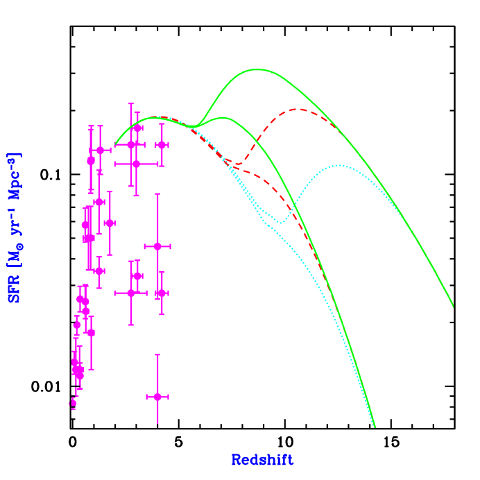
Figure 12: Redshift evolution of the SFR (in $M_{\hbox{$\odot$}}$ per year per comoving Mpc³), adopted from Figure 1 of Barkana & Loeb (2000b) with slight modifications. Points with error bars are observational estimates (compiled by Blain et al. 1999a). Also shown are model predictions for a reionization redshift $z_{\rm reion}=6$ (solid curves), $z_{\rm reion}=8$ (dashed curves), and $z_{\rm reion}=10$ (dotted curves), with a star formation efficiency $\eta=10\%$. In each pair of curves, the upper one is the total SFR, and the lower one is the fraction detectable with NGST  at a limiting point source flux of 0.25 nJy.

Points with error bars in Figure 12 are observational estimates of the cosmic SFR per comoving volume at various redshifts (as compiled by Blain et al. 1999a). We choose $\eta=10\%$ to obtain a rough agreement between the models and these observations at $z\sim 3$–4. An efficiency of order this value is also suggested by observations of the metallicity of the Ly$\alpha$ forest at $z=3$ (Haiman & Loeb 1999b). The SFR curves are roughly proportional to the value of $\eta$. Note that in reality $\eta$ may depend on the halo mass, since the effect of supernova feedback may be more pronounced in small galaxies [see §7 of Barkana & Loeb (2000c) for a review of this topic]. Figure 12 shows a sharp rise in the total SFR at redshifts higher than $z_{\rm reion}$. Although only a fraction of the total SFR can be detected with NGST,  the detectable SFR displays a definite signature of the reionization redshift. However, current observations at lower redshifts demonstrate the observational difficulty in measuring the SFR directly. The redshift evolution of the faint luminosity function provides a clearer, more direct observational signature. We discuss this topic next.

3.2 Galaxy Number Counts

As shown in the previous section, the cosmic star formation history should display a signature of the reionization redshift. Much of the increase in the star formation rate beyond the reionization redshift is due to star formation occurring in very small, and thus faint, galaxies. This evolution in the faint luminosity function constitutes the clearest observational signature of the suppression of star formation after reionization.

Figure 13 shows the predicted redshift distribution in $\Lambda$CDM of galaxies observed with NGST.  The plotted quantity is $dN/dz$, where $N$ is the number of galaxies per NGST  field of view ($4\hbox{${}^{\prime}$}\times 4\hbox{${}^{\prime}$}$). The model predictions are shown for a reionization redshift $z_{\rm reion}=6$ (solid curve), $z_{\rm reion}=8$ (dashed curve), and $z_{\rm reion}=10$ (dotted curve), with a star formation efficiency $\eta=10\%$. All curves assume a point-source detection limit of 0.25 nJy. This plot is updated from Figure 7 of Barkana & Loeb (2000a) in that redshifts above $z_{\rm reion}$ are included.

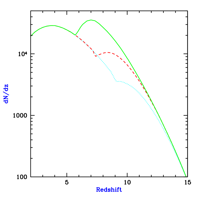
Figure 13: Predicted redshift distribution of galaxies observed with NGST,  adopted and modified from Figure 7 of Barkana & Loeb (2000a). The distribution in the $\Lambda$CDM model, with a star formation efficiency $\eta=10\%$, is shown for a reionization redshift $z_{\rm reion}=6$ (solid curve), $z_{\rm reion}=8$ (dashed curve), and $z_{\rm reion}=10$ (dotted curve). The plotted quantity is $dN/dz$, where $N$ is the number of galaxies per NGST  field of view. All curves assume a limiting point source flux of 0.25 nJy.

Clearly, thousands of galaxies are expected to be found at high redshift. This will allow a determination of the luminosity function at many redshift intervals, and thus a measurement of its evolution. As the redshift is increased, the luminosity function is predicted to gradually change shape during the overlap era of reionization. Figure 14 shows the predicted evolution of the luminosity function for various values of $z_{\rm reion}$. This Figure is adopted from Figure 2 of Barkana & Loeb (2000b) with modifications (in the initial mass function, the values of the cosmological parameters, and the plot layout). All curves show $d^{2}N/(dz\ d\ln F_{\nu}^{\rm ps})$, where $N$ is the total number of galaxies in a single field of view of NGST,  and $F_{\nu}^{\rm ps}$ is the limiting point source flux at 0.6–3.5$\mu$m for NGST.  Each panel shows the result for a reionization redshift $z_{\rm reion}=6$ (solid curve), $z_{\rm reion}=8$ (dashed curve), and $z_{\rm reion}=10$ (dotted curve). Figure 14 shows the luminosity function as observed at $z=5$ (upper left panel) and (proceeding clockwise) at $z=7$, $z=9$, and $z=11$. Although our model assigns a fixed luminosity to all halos of a given mass and redshift, in reality such halos would have some dispersion in their merger histories and thus in their luminosities. We thus include smoothing in the plotted luminosity functions. Note the enormous increase in the number density of faint galaxies in a pre-reionization universe. Observing this dramatic increase toward high redshift would constitute a clear detection of reionization and of its major effect on galaxy formation.

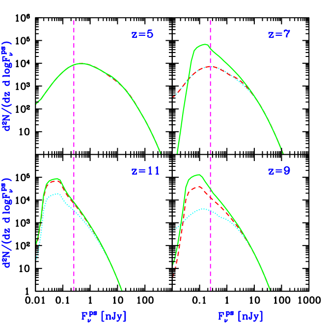
Figure 14: Predicted luminosity function of galaxies at a fixed redshift, adopted and modified from Figure 2 of Barkana & Loeb (2000b). With $\eta=10\%$, the curves show $d^{2}N/(dz\ d\ln F_{\nu}^{\rm ps})$, where $N$ is the total number of galaxies in a single field of view of NGST,  and $F_{\nu}^{\rm ps}$ is the limiting point source flux at 0.6–3.5$\mu$m for NGST.  The luminosity function is shown at $z=5$, $z=7$, $z=9$, and $z=11$, with redshift increasing clockwise starting with the upper left panel. Each case assumes the $\Lambda$CDM model and a reionization redshift $z_{\rm reion}=6$ (solid curves), $z_{\rm reion}=8$ (dashed curves), or $z_{\rm reion}=10$ (dotted curves). The expected NGST  detection limit is shown by the vertical dashed line.

3.3 Quasar Number Counts

Dynamical studies indicate that massive black holes exist in the centers of most nearby galaxies (Richstone et al. 1998; Kormendy & Ho 2000; Kormendy 2000, and references therein). This leads to the profound conclusion that black hole formation is a generic consequence of galaxy formation. The suggestion that massive black holes reside in galaxies and power quasars dates back to the sixties (Zel’dovich 1964; Salpeter 1964; Lynden Bell 1969). Efstathiou & Rees (1988) pioneered the modeling of quasars in the modern context of galaxy formation theories. The model was extended by Haehnelt & Rees (1993) who added more details concerning the black hole formation efficiency and lightcurve. Haiman & Loeb (1998) and Haehnelt, Natarajan, & Rees (1998) extrapolated the model to high redshifts. All of these discussions used the Press-Schechter theory to describe the abundance of galaxy halos as a function of mass and redshift. More recently, Kauffmann & Haehnelt (2000; also Haehnelt & Kauffmann 2000) embedded the description of quasars within semi-analytic modeling of galaxy formation, which uses the extended Press-Schechter formalism to describe the merger history of galaxy halos.

In general, the predicted evolution of the luminosity function of quasars is constrained by the need to match the observed quasar luminosity function at redshifts $z\mathrel{\hbox{\hbox to0.0pt{\hbox{\lower 4.0pt\hbox{$\sim$}}\hss}\hbox{$<$}}}5$, as well as data from the Hubble Deep Field (HDF) on faint point–sources. Prior to reionization, we may assume that quasars form only in galaxy halos with a circular velocity $\mathrel{\hbox{\hbox to0.0pt{\hbox{\lower 4.0pt\hbox{$\sim$}}\hss}\hbox{$>$}}}10~{}{\rm km~{}s^{-1}}$ (or equivalently a virial temperature $\mathrel{\hbox{\hbox to0.0pt{\hbox{\lower 4.0pt\hbox{$\sim$}}\hss}\hbox{$>$}}}10^{4}$ K), for which cooling by atomic transitions is effective. After reionization, quasars form only in galaxies with a circular velocity $\mathrel{\hbox{\hbox to0.0pt{\hbox{\lower 4.0pt\hbox{$\sim$}}\hss}\hbox{$>$}}}50\ {\rm km~{}s^{-1}}$, for which substantial gas accretion from the warm ($\sim 10^{4}$ K) IGM is possible. The limits set by the null detection of quasars in the HDF are consistent with the number counts of quasars which are implied by these thresholds (Haiman, Madau, & Loeb 1999).

For spherical accretion of ionized gas, the bolometric luminosity emitted by a black hole has a maximum value beyond which radiation pressure prevents gas accretion. This Eddington luminosity (Eddington 1926) is derived by equating the radiative repulsive force on a free electron to the gravitational attractive force on an ion in the plasma. Since both forces scale as $r^{-2}$, the limiting Eddington luminosity is independent of radius $r$ in the Newtonian regime, and for gas of primordial composition is given by,

$$L_{E}=1.45\times 10^{46}\left({M_{\rm bh}\over 10^{8}M_{\odot}}\right)~{}{\rm erg~{}s^{-1}}\ ,$$ (8)

where $M_{\rm bh}$ is the black hole mass. Generically, the Eddington limit applies to within a factor of order unity also to simple accretion flows in a non-spherical geometry (Frank, King, & Raine 1992).

The total luminosity of a black hole is related to its mass accretion rate by the radiative efficiency, $\epsilon$,

$$L=\epsilon\dot{M}_{\rm bh}c^{2}.$$ (9)

For accretion through a thin Keplerian disk onto a Schwarzschild (non-rotating) black hole, $\epsilon=5.7\%$, while for a maximally rotating Kerr black hole, $\epsilon=42\%$ (Shapiro & Teukolsky 1983, p. 429). The thin disk configuration, for which these high radiative efficiencies are attainable, exists for $L_{\rm disk}\mathrel{\hbox{\hbox to0.0pt{\hbox{\lower 4.0pt\hbox{$\sim$}}\hss}\hbox{$<$}}}0.5L_{E}$ (Laor & Netzer 1989) .

The accretion time can be defined as

$$\tau={M_{\rm bh}\over{\dot{M}}_{\rm bh}}=4\times 10^{7}~{}{\rm yr}\left(\epsilon\over 0.1\right)\left({L\over L_{E}}\right)^{-1},$$ (10)

This time is comparable to the dynamical time inside the central kpc of a typical galaxy, $t_{\rm dyn}\sim({\rm 1~{}kpc}/100~{}{\rm km~{}s^{-1}})=10^{7}~{}{\rm yr}$. As long as its fuel supply is not limited and $\epsilon$ is constant, a black hole radiating at the Eddington limit will grow its mass exponentially with an $e$–folding time equal to $\tau$. The fact that $\tau$ is much shorter than the age of the universe even at high redshift implies that black hole growth is mainly limited by the feeding rate ${\dot{M}}_{\rm bh}(t)$, or by the total fuel reservoir, and not by the Eddington limit.

The “simplest model” for quasars involves the following three assumptions (Haiman & Loeb 1998):

(i) A fixed fraction of the baryons in each “newly formed” galaxy ends up making a central black hole.

(ii) Each black hole shines at its maximum (Eddington) luminosity for a universal amount of time.

(iii) All black holes share the same emission spectrum during their luminous phase (approximated, e.g., by the average quasar spectrum measured by Elvis et al. 1994).

Note that these assumptions relate only to the most luminous phase of the black hole accretion process, and they may not be valid during periods when the radiative efficiency or the mass accretion rate is very low. At high redshifts the number of “newly formed” galaxies can be estimated based on the time-derivative of the Press-Schechter mass function, since the collapsed fraction of baryons is small and most galaxies form out of the unvirialized IGM. Haiman & Loeb (1998, 1999a) have shown that the above simple prescription provides an excellent fit to the observed evolution of the luminosity function of bright quasars between redshifts $2.6<z<4.5$ (see the analytic description of the existing data in Pei 1995). The observed decline in the abundance of bright quasars (Schneider, Schmidt, & Gunn 1991; Pei 1995) results from the deficiency of massive galaxies at high redshifts. Consequently, the average luminosity of quasars declines with increasing redshift. The required ratio between the mass of the black hole and the total baryonic mass inside a halo is $M_{\rm bh}/M_{\rm gas}=10^{-3.2}{\Omega_{m}}/\Omega_{b}=5.5\times 10^{-3}$, comparable to the typical value of $\sim 2$–$6\times 10^{-3}$ found for the ratio of black hole mass to spheroid mass in nearby elliptical galaxies (Magorrian et al. 1998; Kormendy 2000). The required lifetime of the bright phase of quasars is $\sim 10^{6}$ yr. Figure 15 shows the most recent prediction of this model (Haiman & Loeb 1999a) for the number counts of high-redshift quasars, taking into account the above-mentioned thresholds for the circular velocities of galaxies before and after reionization.

We do, however, expect a substantial intrinsic scatter in the ratio $M_{\rm bh}/M_{\rm gas}$. Observationally, the scatter around the average value of $\log_{10}(M_{\rm bh}/L)$ is 0.3 (Magorrian et al. 1998), while the standard deviation in $\log_{10}(M_{\rm bh}/M_{\rm gas})$ has been found to be $\sigma\sim 0.5$. Such an intrinsic scatter would flatten the predicted quasar luminosity function at the bright end, where the luminosity function is steeply declining. However, Haiman & Loeb (1999a) have shown that the flattening introduced by the scatter can be compensated for through a modest reduction in the fitted value for the average ratio between the black hole mass and halo mass by $\sim 50\%$ in the relevant mass range ($10^{8}~{}{\rm M_{\odot}}\mathrel{\hbox{\hbox to0.0pt{\hbox{\lower 4.0pt\hbox{$\sim$}}\hss}\hbox{$<$}}}M_{\rm bh}\mathrel{\hbox{\hbox to0.0pt{\hbox{\lower 4.0pt\hbox{$\sim$}}\hss}\hbox{$<$}}}10^{10}~{}{\rm M_{\odot}}$).

In reality, the relation between the black hole and halo masses may be more complicated than linear. Models with additional free parameters, such as a non-linear (mass and redshift dependent) relation between the black hole and halo mass, can also produce acceptable fits to the observed quasar luminosity function (Haehnelt et al. 1998). The nonlinearity in a relation of the type $M_{\rm bh}\propto M_{\rm halo}^{\alpha}$ with $\alpha>1$, may be related to the physics of the formation process of low–luminosity quasars(Haehnelt et al. 1998; Silk & Rees 1998), and can be tuned so as to reproduce the black hole reservoir with its scatter in the local universe (Cattaneo, Haehnelt, & Rees 1999). Recently, a tight correlation between the masses of black holes and the velocity dispersions of the bulges in which they reside, $\sigma$, was identified in nearby galaxies. Ferrarese & Merritt (2000; see also Merritt & Ferrarese 2000) inferred a correlation of the type $M_{\rm bh}\propto\sigma^{4.72\pm 0.36}$, based on a selected sample of a dozen galaxies with reliable $M_{\rm bh}$ estimates, while Gebhardt et al. (2000a,b) have found a somewhat shallower slope, $M_{\rm bh}\propto\sigma^{3.75(\pm 0.3)}$ based on a significantly larger sample. A non-linear relation of $M_{\rm bh}\propto\sigma^{5}\propto M_{\rm halo}^{5/3}$ has been predicted by Silk & Rees (2000) based on feedback considerations, but the observed relation also follows naturally in the standard semi-analytic models of galaxy formation (Haehnelt & Kauffmann 2000).

Figure 16 shows the predicted number counts in the “simplest model” described above (Haiman & Loeb 1999a), normalized to a $5^{\prime}\times 5^{\prime}$ field of view. Figure 16 shows separately the number per logarithmic flux interval of all objects with redshifts $z>5$ (thin lines), and $z>10$ (thick lines). The number of detectable sources is high; NGST  will be able to probe of order $100$ quasars at $z>10$, and $\sim 200$ quasars at $z>5$ per $5^{\prime}\times 5^{\prime}$ field of view. The bright–end tail of the number counts approximately follows a power law, with $dN/dF_{\nu}\propto F_{\nu}^{-2.5}$. The dashed lines show the corresponding number counts of “star–clusters”, assuming that each halo shines due to a starburst that converts a fraction of 2% (long–dashed) or 20% (short–dashed) of the gas into stars.

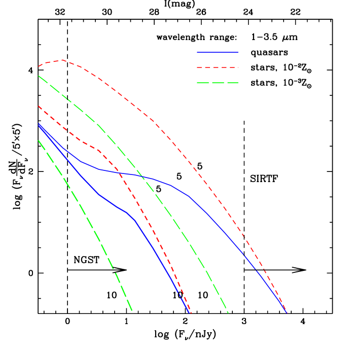
Figure 15: Infrared number counts of quasars (averaged over the wavelength interval of $1$–$3.5\mu$m) based on the “simplest quasar model” of Haiman & Loeb (1999b). The solid curves refer to quasars, while the long/short dashed curves correspond to star clusters with low/high normalization for the star formation efficiency. The curves labeled “5” or “10” show the cumulative number of objects with redshifts above $z=5$ or 10.

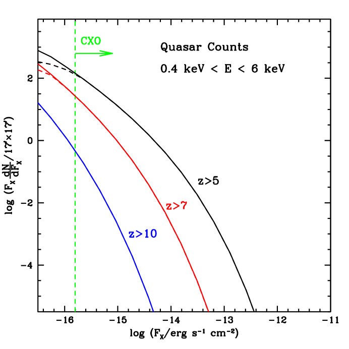
Figure 16: Total number of quasars with redshift exceeding $z=5$, $z=7$, and $z=10$ as a function of observed X-ray flux in the CXO detection band (from Haiman & Loeb 1999a). The numbers are normalized per $17^{\prime}\times 17^{\prime}$ area of the sky. The solid curves correspond to a cutoff in circular velocity for the host halos of $v_{\rm circ}\geq 50~{}{\rm km~{}s^{-1}}$, the dashed curves to a cutoff of $v_{\rm circ}\geq 100~{}{\rm km~{}s^{-1}}$. The vertical dashed line shows the CXO sensitivity for a 5$\sigma$ detection of a point source in an integration time of $5\times 10^{5}$ seconds.

Similar predictions can be made in the X-ray regime. Figure 16 shows the number counts of high-redshift X-ray quasars in the above “simplest model”. This model fits the X-ray luminosity function of quasars at $z\sim 3.5$ as observed by ROSAT (Miyaji, Hasinger, & Schmidt 2000), using the same parameters necessary to fit the optical data (Pei 1995). Deep optical or infrared follow-ups on deep images taken with the Chandra X-ray satellite (CXO; see, e.g., Mushotzky et al. 2000; Barger et al. 2000; Giaconni et al. 2000) will be able to test these predictions in the relatively near future.

The “simplest model” mentioned above predicts that black holes and stars make comparable contributions to the ionizing background prior to reionization. Consequently, the reionization of hydrogen and helium is predicted to occur roughly at the same epoch. A definitive identification of the He II reionization redshift will provide another powerful test of this model. Further constraints on the lifetime of the active phase of quasars may be provided by future measurements of the clustering properties of quasars (Haehnelt et al. 1998; Martini & Weinberg 2000; Haiman & Hui 2000).

3.4 High-Redshift Supernovae

The detection of galaxies and quasars becomes increasingly difficult at a higher redshift. This results both from the increase in the luminosity distance and the decrease in the average galaxy mass with increasing redshift. It therefore becomes advantageous to search for transient sources, such as supernovae or $\gamma$-ray bursts, as signposts of high-redshift galaxies (Miralda-Escudé & Rees 1997). Prior to or during the epoch of reionization, such sources are likely to outshine their host galaxies.

The IGM is observed to be enriched with metals at redshifts $z\mathrel{\hbox{\hbox to0.0pt{\hbox{\lower 4.0pt\hbox{$\sim$}}\hss}\hbox{$<$}}}5$. Identification of C IV, Si IV and O VI absorption lines which correspond to Ly$\alpha$ absorption lines in the spectra of high-redshift quasars has revealed that the low-density IGM has been enriched to a metal abundance (by mass) of $Z_{\rm IGM}\sim 10^{-2.5(\pm 0.5)}Z_{\odot}$, where $Z_{\odot}=0.019$ is the solar metallicity (Meyer & York 1987; Tytler et al. 1995; Songaila & Cowie 1996; Lu et al 1998; Cowie & Songaila 1998; Songaila 1997; Ellison et al. 2000). The metal enrichment has been clearly identified down to H I column densities of $\sim 10^{14.5}~{}{\rm cm^{-2}}$. The metals detected in the IGM signal the existence of supernova (SN) explosions at redshifts $z\mathrel{\hbox{\hbox to0.0pt{\hbox{\lower 4.0pt\hbox{$\sim$}}\hss}\hbox{$>$}}}5$. Since each SN produces an average of $\sim 1M_{\odot}$ of heavy elements (Woosley & Weaver 1995), the inferred metallicity of the IGM implies that there should be a supernova at $z\mathrel{\hbox{\hbox to0.0pt{\hbox{\lower 4.0pt\hbox{$\sim$}}\hss}\hbox{$>$}}}5$ for each $\sim 1.7\times 10^{4}M_{\odot}\times(Z_{\rm IGM}/10^{-2.5}Z_{\odot})^{-1}$ of baryons in the universe. We can therefore estimate the total supernova rate, on the entire sky, necessary to produce these metals at $z\sim 5$. In a flat ${\Omega_{m}}=0.3$ cosmology, the total supernova rate across the entire sky at $z\mathrel{\hbox{\hbox to0.0pt{\hbox{\lower 4.0pt\hbox{$\sim$}}\hss}\hbox{$>$}}}5$ is estimated to be (Miralda-Escudé & Rees 1997) roughly one SN per square arcminute per year, if $Z_{\rm IGM}=10^{-2.5}Z_{\odot}$.

The actual SN rate at a given observed flux threshold is determined by the star formation rate per unit comoving volume as a function of redshift and the initial mass function of stars (e.g., Madau, della Valle, & Panagia 1998; Woods & Loeb 1998; Sullivan et al. 2000) Figure 17 shows the predicted SN rate as a function of limiting flux in various bands (Woods & Loeb 1998), based on the comoving star formation rate as a function of redshift that was determined empirically by Madau (1997). The actual star formation rate may be somewhat higher due to corrections for dust extinction (for a recent compilation of current data, see Blain & Natarajan 2000). The dashed lines correspond to Type Ia SNe and the dotted lines to Type II SNe. For comparison, the solid lines indicate two crude estimates for the rate of $\gamma$–ray burst afterglows, which are discussed in detail in the next section.

Figure 17: Predicted cumulative rate $\dot{N}(>F_{\nu})$ per year per square degree of supernovae at four wavelengths, corresponding to the $K$, $R$, $B$, and $U$ bands (from Woods & Loeb 1998). The broken lines refer to different supernova types, namely SNe Ia (dashed curves) and SNe II (dotted curves). For comparison, the solid curves show estimates for the rates of gamma-ray burst (GRB) afterglows; the lower solid curve assumes the best-fit rate and luminosity for GRB sources which trace the star formation history (Wijers et al. 1998), while the upper solid curve assumes the best-fit values for a non-evolving GRB population.

The above SN rate is appropriate for a threshold experiment, one which monitors the sky continuously and triggers when the detected flux exceeds a certain value, and hence identifies the most distant sources only when they are near their peak flux. For search strategies which involve taking a series of “snapshots” of a field and looking for variations in the flux of sources in successive images, one does not necessarily detect most sources near their peak flux. In this case, we can estimate the total  number of events (i.e., not  per unit time) brighter than $F_{\nu}$ at a given observed wavelength. A simple estimate uses the rest-frame duration over which an event will be brighter than the limiting flux $F_{\nu}$ at redshift $z$. This is a naive estimate of the so-called “control time”; in practice, the effective duration over which an event can be observed is shorter, owing to the image subtraction technique, host galaxy magnitudes, and a number of other effects which reduce the detection efficiency (Pain et al. 1996).

Supernovae also produce dust which could process the emission spectrum of galaxies. Although produced in galaxies, the dust may be expelled together with the metals out of galaxies by supernova-driven winds. Loeb & Haiman (1997) have shown that if each supernova produces $\sim 0.3\,M_{\odot}$ of Galactic dust, and some of the dust is expelled together with metals out of the shallow potential wells of the early dwarf galaxies, then the optical depth for extinction by intergalactic dust may reach a few tenths at $z\sim 10$ for observed wavelengths of $\sim 0.5$–$1\,\mu$m [see Todini & Ferrara (2000) for a detailed discussion on the production of dust in primordial Type II SNe]. The opacity in fact peaks in this wavelength band since at $z\sim 10$ it corresponds to rest-frame UV, where normal dust extinction is most effective. In these estimates, the amplitude of the opacity is calibrated based on the observed metallicity of the IGM at $z\mathrel{\hbox{\hbox to0.0pt{\hbox{\lower 4.0pt\hbox{$\sim$}}\hss}\hbox{$<$}}}5$. The intergalactic dust absorbs the UV background at the reionization epoch and re-radiates it at longer wavelengths. The flux and spectrum of the infrared background which is produced at each redshift depends sensitively on the distribution of dust around the ionizing sources, since the deviation of the dust temperature from the microwave background temperature depends on the local flux of UV radiation that it is exposed to. For reasonable choices of parameters, dust could lead to a significant spectral distortion of the microwave background spectrum that could be measured by a future spectral mission, going beyond the upper limit derived by the COBE satellite (Fixsen et al. 1996).

The metals produced by supernovae may also yield strong molecular line emission. Silk & Spaans (1997) pointed out that the rotational line emission of CO by starburst galaxies is enhanced at high redshift due to the increasing temperature of the cosmic microwave background, which affects the thermal balance and the level populations of the atomic and molecular species. They found that the future Millimeter Array (MMA) could detect a starburst galaxy with a star formation rate of $\sim 30\,{\rm M_{\odot}~{}yr^{-1}}$ equally well at $z=5$ and $z=30$ because of the increasing cosmic microwave background temperature with redshift. Line emission may therefore be a more powerful probe of the first bright galaxies than continuum emission by dust.

3.5 High-Redshift Gamma Ray Bursts

The past decade has seen major observational breakthroughs in the study of Gamma Ray Burst (GRB) sources. The Burst and Transient Source Experiment (BATSE) on board the Compton Gamma Ray Observatory (Meegan et al. 1992) showed that the GRB population is distributed isotropically across the sky, and that there is a deficiency of faint GRBs relative to a Euclidean distribution. These were the first observational clues indicating a cosmological distance scale for GRBs. The localization of GRBs by X-ray observations with the BeppoSAX satellite (Costa et al. 1997) allowed the detection of afterglow emission at optical (e.g., van Paradijs et al. 1997) and radio (e.g., Frail et al. 1997) wavelengths up to more than a year following the events (Fruchter et al. 1999; Frail et al. 1999). The afterglow emission is characterized by a broken power-law spectrum with a peak frequency that declines with time. The radiation is well-fitted by a model consisting of synchrotron emission from a decelerating blast wave (Blandford & McKee 1976), created by the GRB explosion in an ambient medium, with a density comparable to that of the interstellar medium of galaxies (Waxman 1997; Sari, Piran, & Narayan 1998; Wijers & Galama 1999; Mészáros 1999; but see also Chevalier & Li 2000). The detection of spectral features, such as metal absorption lines in some optical afterglows (Metzger et al. 1997) and emission lines from host galaxies (Kulkarni et al. 2000), allowed an unambiguous identification of the cosmological distance-scale to these sources.

The nature of the central engine of GRBs is still unknown. Since the inferred energy release, in cases where it can be securely calibrated (Freedman & Waxman 1999; Frail et al. 2000), is comparable to that in a supernova, $\sim 10^{51}~{}{\rm erg}$, most popular models relate GRBs to stellar remnants such as neutron stars or black holes (Eichler et al. 1989; Narayan, Paczyński, & Piran 1992; Paczyński 1991; Usov 1992; Mochkovitch et al. 1993; Paczyński 1998; MacFadyen & Woosley 1999). Recently it has been claimed that the late evolution of some rapidly declining optical afterglows shows a component which is possibly associated with supernova emission (e.g., Bloom et al. 1999; Reichart 1999). If the supernova association is confirmed by detailed spectra of future afterglows, the GRB phenomenon will be linked to the terminal evolution of massive stars.

Any association of GRBs with the formation of single compact stars implies that the GRB rate should trace the star formation history of the universe (Totani 1997; Sahu et al. 1997; Wijers et al. 1998; but see Krumholz, Thorsett & Harrison 1998). Owing to their high brightness, GRB afterglows could in principle be detected out to exceedingly high redshifts. Just as for quasars, the broad-band emission of GRB afterglows can be used to probe the absorption properties of the IGM out to the reionization epoch at redshift $z\sim 10$. Lamb & Reichart (2000) extrapolated the observed gamma-ray and afterglow spectra of known GRBs to high redshifts and emphasized the important role that their detection could play in probing the IGM. In particular, the broad-band afterglow emission can be used to probe the ionization and metal-enrichment histories of the intervening intergalactic medium during the epoch of reionization.

Ciardi & Loeb (2000) showed that unlike other sources (such as galaxies and quasars), which fade rapidly with increasing redshift, the observed infrared flux from a GRB afterglow at a fixed observed age is only a weak function of its redshift (Figure 18). A simple scaling of the long-wavelength spectra and the temporal evolution of afterglows with redshift implies that at a fixed time-lag after the GRB in the observer’s frame, there is only a mild change in the observed flux at infrared or radio wavelengths with increasing redshift. This results in part from the fact that afterglows are brighter at earlier times, and that a given observed time refers to an earlier intrinsic time in the source frame as the source redshift increases. The “apparent brightening” of GRB afterglows with redshift could be further enhanced by the expected increase with redshift of the mean density of the interstellar medium of galaxies (Wood & Loeb 2000). Figure 19 shows the expected number counts of GRB afterglows, assuming that the GRB rate is proportional to the star formation rate and that the characteristic energy output of GRBs is $\sim 10^{52}~{}{\rm erg}$ and is isotropic. The figure implies that at any time there should be of order $\sim 15$ GRBs with redshifts $z\mathrel{\hbox{\hbox to0.0pt{\hbox{\lower 4.0pt\hbox{$\sim$}}\hss}\hbox{$>$}}}5$ across the sky which are brighter than $\sim 100$ nJy at an observed wavelength of $\sim 2\mu$m. The infrared spectrum of these sources could be measured with NGST  as a follow-up on their early X-ray localization with $\gamma$-ray or X-ray detectors. Prior to reionization, the spectrum of GRB afterglows could reveal the long sought-after Gunn-Peterson trough (Gunn & Peterson 1965) due to absorption by the neutral intergalactic medium.

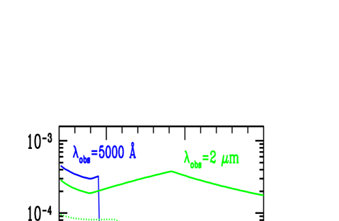
Figure 18: Observed flux from a $\gamma$-ray burst afterglow as a function of redshift (from Ciardi & Loeb 2000). The two sets of curves refer to a photon frequency $\nu=6\times 10^{14}$ Hz ($\lambda_{obs}=5000$ Å, thin lines) and $\nu=1.5\times 10^{14}$ Hz ($\lambda_{obs}=2\mu$m, thick lines). Each set shows different observed times after the GRB trigger; from top to bottom: 1 hour (solid line), 1 day (dotted) and 10 days (dashed). The sharp suppression for 5000 Å  at $z\mathrel{\hbox{\hbox to0.0pt{\hbox{\lower 4.0pt\hbox{$\sim$}}\hss}\hbox{$>$}}}4.5$ is due to IGM absorption.

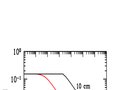
Figure 19: Predicted number of GRB afterglows per square degree with observed flux greater than $F$, at several different observed wavelengths (from Ciardi & Loeb 2000). From right to left, the observed wavelength equals 10 cm, 1 mm, 2 $\mu$m and 5000 Å.

The predicted GRB rate and flux are subject to uncertainties regarding the beaming of the emission. The beaming angle may vary with observed time due to the decline with time of the Lorentz factor $\gamma(t)$ of the emitting material. As long as the Lorentz factor is significantly larger than the inverse of the beaming angle (i.e., $\gamma\mathrel{\hbox{\hbox to0.0pt{\hbox{\lower 4.0pt\hbox{$\sim$}}\hss}\hbox{$>$}}}\theta^{-1}$), the afterglow flux behaves as if it were emitted by a spherically-symmetric fireball with the same explosion energy per unit solid angle. However, the lightcurve changes as soon as $\gamma$ declines below $\theta^{-1}$, due to the lateral expansion of the jet (Rhoads 1997, 1999a,b; Panaitescu & Meszaros 1999). Finally, the isotropization of the energy ends when the expansion becomes sub-relativistic, at which point the remnant recovers the spherically-symmetric Sedov-Taylor evolution for the total energy output. When $\gamma\sim 1$, the emission occurs from a roughly spherical fireball with the effective explosion energy per solid angle reduced by a factor of $(2\pi\theta^{2}/4\pi)$ relative to that at early times, representing the fraction of sky around the GRB source which is illuminated by the initial two (opposing) jets of angular radius $\theta$ (see Ciardi & Loeb 2000 for the impact of this effect on the number counts). The calibration of the GRB event rate per comoving volume, based on the number counts of GRBs (Wijers et al. 1998), is inversely proportional to this factor.

The main difficulty in using GRBs as probes of the high-redshift universe is that they are rare, and hence their detection requires surveys which cover a wide area of the sky. The simplest strategy for identifying high-redshift afterglows is through all-sky surveys in the $\gamma$-ray or X-ray regimes. In particular, detection of high-redshift sources will become feasible with the high trigger rate provided by the forthcoming Swift  satellite, to be launched in 2003 (see http://swift.gsfc.nasa.gov/, for more details). Swift  is expected to localize $\sim$300 GRBs per year, and to re-point within 20–70 seconds its on-board X-ray and UV-optical instrumentation for continued afterglow studies. The high-resolution GRB coordinates obtained by Swift  will be transmitted to Earth within $\sim$50 seconds. Deep follow-up observations will then be feasible from the ground or using the highly-sensitive infrared instruments on board NGST.  Swift  will be sufficiently sensitive to trigger on the $\gamma$-ray emission from GRBs at redshifts $z\mathrel{\hbox{\hbox to0.0pt{\hbox{\lower 4.0pt\hbox{$\sim$}}\hss}\hbox{$>$}}}10$ (Lamb & Reichart 2000).

4 OBSERVATIONAL PROBES OF THE EPOCH OF REIONIZATION

4.1 Inferring the Reionization Redshift Using Ly$\alpha$ Photons

The scattering cross-section of the Ly$\alpha$ resonance line by neutral hydrogen is given in Peebles (1993, §23). We consider a source at a redshift $z_{s}$ beyond the redshift of reionization $z_{i}$, and the corresponding scattering optical depth of a uniform, neutral IGM between the source and the reionization redshift. The optical depth is in general given by integrating the absorption along the line of sight. At wavelengths longer than Ly$\alpha$ at the source, the optical depth obtains a small value; these photons redshift away from the line center along its red wing and never resonate with the line core on their way to the observer. Considering only this regime of the absorption wing leads to an analytical result for the red damping wing of the Gunn-Peterson trough (Miralda-Escudé 1998).

At wavelengths corresponding to the Ly$\alpha$ resonance between the source redshift and the reionization redshift, $(1+z_{i})\lambda_{\alpha}\leq\lambda_{\rm obs}\leq(1+z_{s})\lambda_{\alpha}$, the optical depth is given by the standard formula of Gunn & Peterson (1965). Since this optical depth is $\sim 10^{5}$, the flux from the source is entirely suppressed in this regime. Similarly, the Ly$\beta$ resonance produces another trough at wavelengths $(1+z_{i})\lambda_{\beta}\leq\lambda\leq(1+z_{s})\lambda_{\beta}$, where $\lambda_{\beta}=(27/32)\lambda_{\alpha}=1026\,$Å, and the same applies to the higher Lyman series lines. If $(1+z_{s})\geq 1.18(1+z_{i})$ then the Ly$\alpha$ and the Ly$\beta$ resonances overlap and no flux is transmitted in-between the two troughs (see Figure 20). The same holds for the higher Lyman-series resonances down to the Lyman limit wavelength of $\lambda_{c}=912$Å.

At wavelengths shorter than $\lambda_{c}$, the photons are absorbed when they photoionize atoms of hydrogen or helium. The bound-free absorption cross-section from the ground state of a hydrogenic ion (including neutral hydrogen singly-ionized helium) is given by Osterbrock (1974). The cross-section for neutral helium is more complicated; when averaged over its narrow resonances it can be fitted to an accuracy of a few percent up to $h\nu=50$ keV by a simple fitting function (Verner et al. 1986).

For rough estimates, the average photoionization cross-section for a mixture of hydrogen and helium with cosmic abundances can be approximated in the range of $54<h\nu\mathrel{\hbox{\hbox to0.0pt{\hbox{\lower 4.0pt\hbox{$\sim$}}\hss}\hbox{$<$}}}10^{3}$ eV as $\sigma_{bf}\approx\sigma_{0}(\nu/\nu_{\rm H,0})^{-3}$, where $\sigma_{0}\approx 6\times 10^{-17}~{}{\rm cm^{2}}$ (Miralda-Escudé 2000). For a source beyond the redshift of reionization, the resulting bound-free optical depth only becomes of order unity in the extreme UV to soft X-rays, around $h\nu\sim 0.1$ keV, a regime which is unfortunately difficult to observe due to Galactic absorption (Miralda-Escudé 2000).

A sketch of the overall spectrum of a source slightly above the reionization redshift, i.e., with $1<[(1+z_{\rm s})/(1+z_{i})]<1.18$, is shown in Figure 20. The transmitted flux between the Gunn-Peterson troughs due to Ly$\alpha$ and Ly$\beta$ absorption is suppressed by the Ly$\alpha$ forest in the post-reionization epoch. Transmission of flux due to H II bubbles in the pre-reionization epoch is expected to be negligible (Miralda-Escudé 1998). The redshift of reionization can be inferred in principle from the spectral shape of the red damping wing (Miralda-Escudé & Rees 1998; Miralda-Escudé 1998) or from the transmitted flux between the Lyman series lines (Haiman & Loeb 1999a). However, these signatures are complicated in reality by damped Ly$\alpha$ systems along the line-of-sight or by the inhomogeneity or peculiar velocity field of the IGM in the vicinity of the source. Moreover, bright sources, such as quasars, tend to ionize their surrounding environment (Wood & Loeb 2000) and the resulting H II region in the IGM could shift the Ly$\alpha$ trough substantially (Cen & Haiman 2000; Madau & Rees 2000).

The inference of the Ly$\alpha$ transmission properties of the IGM from the observed spectrum of high-redshift sources suffers from uncertainties about the precise emission spectrum of these sources, and in particular the shape of their Ly$\alpha$ emission line. The first galaxies and quasars are expected to have pronounced recombination lines of hydrogen and helium due to the lack of dust in their interstellar medium (Oh 1999; Tumlinson & Shull 2000; see also Baltz, Gnedin & Silk 1998). Lines such as $H_{\alpha}$ or the He II 1640 Å  line should reach the observer unaffected by the intervening IGM, since their wavelength is longer than that of the Ly$\alpha$ transition which dominates the IGM opacity (Oh 1999). However, as described above, the situation is different for the Ly$\alpha$ line photons. As long as $z_{s}>z_{i}$, the intervening neutral IGM acts like a fog and obscures the view of the Ly$\alpha$ source [in contrast to the situation with sources at $z_{s}<z_{i}$, where most of the intervening IGM is ionized and only the blue wing of the Ly$\alpha$ line is suppressed by the Ly$\alpha$ forest (see Figure 2)]. Photons which are emitted at the Ly$\alpha$ line center have an initial scattering optical depth of $\sim 10^{5}$ in the surrounding medium.

The Ly$\alpha$ line photons are not destroyed but instead are absorbed and re-emitted. Due to the Hubble expansion of the IGM around the source, the frequency of the photons is slightly shifted by the Doppler effect in each scattering event. As a result, the photons diffuse in frequency to the red side of the Ly$\alpha$ resonance. Eventually, when their net frequency redshift is sufficiently large, they escape and travel freely towards the observer (see figure 21). As a result, the source creates a faint Ly$\alpha$ halo on the sky. The well-defined radiative transfer problem of a point source of Ly$\alpha$ photons embedded in a uniform neutral IGM was solved by Loeb & Rybicki (1999). The Ly$\alpha$ halo can be simply characterized by the frequency redshift relative to the line center, $(\nu-\nu_{\alpha})$, which is required in order to make the optical depth from the source equal to unity. At $z_{s}\sim 10$, this frequency shift of $\nu_{\star}\sim 1\times 10^{13}$ Hz relative to the line center corresponds to a Doppler velocity of $v\sim 10^{3}~{}{\rm km~{}s^{-1}}$. The halo size is then defined by the corresponding proper distance from the source at which the Hubble velocity provides a Doppler shift of this magnitude, $r_{\star}\sim 1~{}{\rm Mpc}$. Typically, the Ly$\alpha$ halo of a source at $z_{\rm s}\sim 10$ occupies an angular radius of $\sim 15^{\prime\prime}$ on the sky and yields an asymmetric line profile as shown in Figure 21. The scattered photons are highly polarized and so the shape of the halo would be different if viewed through a polarization filter (Rybicki & Loeb 1999).

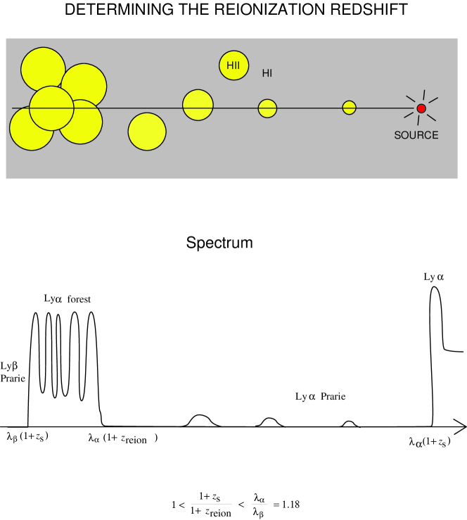
Figure 20: Sketch of the expected spectrum of a source at a redshift $z_{s}$ slightly above the reionization redshift $z_{i}$. The transmitted flux due to H II bubbles in the pre-reionization era and the Ly$\alpha$ forest in the post-reionization era is exaggerated for illustration.

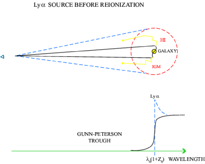
Figure 21: Loeb-Rybicki halos: Scattering of Ly$\alpha$ line photons from a galaxy embedded in the neutral intergalactic medium prior to reionization. The line photons diffuse in frequency due to the Hubble expansion of the surrounding medium and eventually redshift out of resonance and escape to infinity. A distant observer sees a Ly$\alpha$ halo surrounding the source, along with a characteristically asymmetric line profile. The observed line should be broadened and redshifted by about one thousand ${\rm km~{}s^{-1}}$ relative to other lines (such as H_α) emitted by the galaxy.

Detection of the diffuse Ly$\alpha$ halos around bright high redshift sources (which are sufficiently rare so that their halos do not overlap) would provide a unique tool for probing the distribution and the velocity field of the neutral intergalactic medium before the epoch of reionization. The Ly$\alpha$ sources serve as lamp posts which illuminate the surrounding H I fog. On sufficiently large scales where the Hubble flow is smooth and the gas is neutral, the Ly$\alpha$ brightness distribution can be used to determine the cosmological mass densities of baryons and matter. Due to their low surface brightness, the detection of Ly$\alpha$ halos through a narrow-band filter is much more challenging than direct observation of their sources at somewhat longer wavelengths. However, NGST  might be able to detect the Ly$\alpha$ halos around sources as bright as the quasar discovered by Fan et al. (2000) at $z=5.8$ or the galaxy discovered by Hu et al. (1999) at $z=5.74$, even if these sources were moved out to $z\sim 10$ (see §4 in Loeb & Rybicki 1999). The disappearance of Ly$\alpha$ halos below a certain redshift can be used to determine $z_{i}$.

4.2 21 cm Tomography Of The Reionization Epoch

The ground state of hydrogen exhibits hyperfine spitting involving the spins of the proton and the electron. The state with parallel spins (the triplet state) has a slightly higher energy than the state with anti-parallel spins (the singlet state). The 21 cm line associated with the spin-flip transition from the triplet to the singlet state is often used to detect neutral hydrogen in the local universe. At high redshift, the occurrence of a neutral pre-reionization IGM offers the prospect of detecting the first sources of radiation and probing the reionization era by mapping the 21 cm emission from neutral regions. While its energy density is estimated to be only a $1\%$ correction to that of the CMB, the redshifted 21 cm emission should display angular structure as well as frequency structure due to inhomogeneities in the gas density field (Hogan & Rees 1979; Scott & Rees 1990), hydrogen ionized fraction, and spin temperature (Madau, Meiksin, & Rees 1997). Some of the resulting signatures during the pre-overlap phase of reionization (§2.3) and during the overlap phase are discussed by Tozzi et al. (2000) and Shaver et al. (1999), respectively. Also, the 21 cm signatures have been explored in a numerical simulation by Gnedin & Ostriker (1997). Indeed, a detailed mapping of H II regions as a function of redshift is possible in principle, and should be within the reach of proposed instruments such as the Square Kilometer Array (hereafter SKA; see Taylor & Braun 1999). Serious technical challenges and foreground contamination must, however, be overcome even for an initial detection of the reionization signal.

The basic physics of the hydrogen spin transition is determined as follows (for a more detailed treatment, see Madau et al. 1997). The ground-state hyperfine levels of hydrogen tend to thermalize with the CMB background, making the IGM unobservable. If other processes shift the hyperfine level populations away from thermal equilibrium, then the gas becomes observable against the CMB in emission or in absorption. The energy of the 21 cm transition is $E_{21}=5.9\times 10^{-6}$ eV, corresponding to a frequency of 1420 MHz. In the presence of the CMB alone, the spin states reach thermal equilibrium on a timescale which is much shorter than the age of the universe at all redshifts after cosmological recombination.

The IGM is observable when the kinetic temperature of the gas differs from $T_{\rm CMB}$ and an effective mechanism couples the hyperfine levels to the gas temperature. Although collisional de-excitation of the triplet level (Purcell & Field 1956) is a possible mechanism, in the low-density IGM the dominant mechanism is scattering by Ly$\alpha$ photons (Wouthuysen 1952; Field 1958). Continuum UV photons produced by early radiation sources redshift by the Hubble expansion into the local Ly$\alpha$ line at a lower redshift. These photons mix the spin states via the Wouthuysen-Field process whereby an atom initially in the $n=1$ state absorbs a Ly$\alpha$ photon, and the spontaneous decay which returns it from $n=2$ to $n=1$ can result in a final spin state which is different from the initial one. Efficient thermalization of the hyperfine levels occurs above a particular critical scattering rate (Madau et al. 1997).

Assuming such efficient thermalization, a heated patch of neutral hydrogen at the mean density is observed at a differential antenna temperature $\delta T_{b}$ relative to the CMB given by Madau et al. (1997). In overdense regions, the observed $\delta T_{b}$ is proportional to the overdensity, and in partially ionized regions $\delta T_{b}$ is proportional to the neutral fraction. At high temperatures, the IGM is observed in emission at a level ($\delta T_{b}\sim 28\,{\rm mK}$) that is independent of temperature. On the other hand, a cool IGM is observed in absorption at a level that increases with temperature and becomes larger than the maximum $\delta T_{b}$ observable in emission. As a result, a number of cosmic events are expected to leave observable signatures in the redshifted 21 cm line.

Since the CMB temperature is only $2.73(1+z)$ K, even relatively inefficient heating mechanisms are expected to heat the IGM above $T_{\rm CMB}$ well before reionization. Possible preheating sources include soft X-rays from early quasars or star-forming regions, as well as thermal bremsstrahlung from ionized gas in collapsing halos. However, even the radiation from the first stars may suffice for an early preheating. Only $\sim 10\%$ of the present-day global star formation rate is required (Madau et al. 1997) for a sufficiently strong Ly$\alpha$ background which produces a scattering rate above the thermalization rate. Such a background produces absorption, since the kinetic gas temperature is initially lower than $T_{\rm CMB}$ because of adiabatic expansion. Thus, the entire IGM can be seen in absorption, but the IGM is then heated above $T_{\rm CMB}$ in $\sim 10^{8}$ yr (Madau et al. 1997) by the atomic recoil in the repeated resonant Ly$\alpha$ scattering. According to §3.1 (also compare Gnedin 2000a), the required level of star formation is expected to be reached already at $z\sim 20$, with the entire IGM heated well above the CMB by the time overlap begins at $z\sim 10$. Thus, although the initial absorption signal is in principle detectable with the SKA (Tozzi et al. 2000), it likely occurs at $\mathrel{\hbox{\hbox to0.0pt{\hbox{\lower 4.0pt\hbox{$\sim$}}\hss}\hbox{$<$}}}100$ MHz where Earth-based radio interference is highly problematic.

As individual ionizing sources turn on in the pre-overlap stage of reionization, the resulting H II bubbles may be individually detectable if they are produced by rare and luminous sources such as quasars. If the H II region expands into an otherwise unperturbed IGM, then the expanding shell can be mapped as follows (Tozzi et al. 2000). The H II region itself, of course, shows neither emission nor absorption. Outside the ionized bubble, a thin shell of neutral gas is heated above the CMB temperature and shows up in emission. A much thicker outer shell is cooler than the CMB due to adiabatic expansion, and it produces absorption. Finally, at large distances from the quasar, the gas approaches $T_{\rm CMB}$ as the quasar radiation weakens. For a quasar with an ionizing intensity of $10^{57}$ photons s^-1 observed after $\sim 10^{7}$ yr with $2\hbox{${}^{\prime}$}$ resolution and 1 MHz bandwidth, the signal ranges from -3 to 3 $\mu$Jy per beam (Tozzi et al. 2000). Mapping such regions would convey information on the quasar number density, ionizing intensity, opening angle, and on the density distribution in the surrounding IGM. Note, however, that an H II region which forms at a redshift approaching overlap expands into a preheated IGM. In this case, the H II region itself still appears as a hole in an otherwise emitting medium, but the quasar-induced heating is not probed, and there is no surrounding region of absorption to supply an enhanced contrast.

At redshifts approaching overlap, the IGM should be almost entirely neutral but also much hotter than the CMB.. In this redshift range there should still be an interesting signal due to density fluctuations. The same cosmic network of sheets and filaments that gives rise to the Ly$\alpha$ forest observed at $z\mathrel{\hbox{\hbox to0.0pt{\hbox{\lower 4.0pt\hbox{$\sim$}}\hss}\hbox{$<$}}}5$ should lead to fluctuations in the 21 cm brightness temperature at higher redshifts. At 150 MHz ($z=8.5$), for observations with a bandwidth of 1 MHz, the root mean square fluctuation should be $\sim 10$ mK at $1\hbox{${}^{\prime}$}$, decreasing with scale (Tozzi et al. 2000).

A further signature, observable over the entire sky, should mark the overlap stage of reionization. During overlap, the IGM is transformed from being a neutral, preheated and thus emitting gas, to being almost completely ionized. This disappearance of the emission over a relatively narrow redshift range can be observed as a drop in the brightness temperature at the frequencies corresponding to the latter stages of overlap (Shaver et al. 1999). This exciting possibility, along with those mentioned above, face serious challenges in terms of signal contamination and calibration. The noise sources include galactic and extragalactic emission sources, as well as terrestrial interference, and all of these foregrounds must be modeled and accurately removed in order to observe the fainter cosmological signal (see Shaver et al. 1999 for a detailed discussion). For the overlap stage in particular, the sharpness of the spectral feature is the key to its detectability, but it may be significantly smoothed by inhomogeneities in the IGM.

4.3 Effect of Reionization on CMB Anisotropies

In standard cosmological models, the early universe was hot and permeated by a nearly uniform radiation bath. At $z\sim 1200$ the free protons and electrons recombined to form hydrogen atoms, and most of the photons last scattered as the scattering cross-section dropped precipitously. These photons, observed today as the Cosmic Microwave Background (CMB), thus yield a snapshot of the state of the universe at that early time. Small fluctuations in the density, velocity, and gravitational potential lead to observed anisotropies (e.g., Bennett et al. 1996) that can be analyzed to yield a great wealth of information on the matter content of the universe and on the values of the cosmological parameters (e.g., Hu 1995).

Reionization can alter the anisotropy spectrum, by erasing some of the primary anisotropy imprinted at recombination, and by generating additional secondary fluctuations that could be used to probe the era of reionization itself (see Haiman & Knox 1999 for a review). The primary anisotropy is damped since the rescattering leads to a blending of photons from initially different lines of sight. Furthermore, not all the photons scatter at the same time, rather the last scattering surface has a finite thickness. Perturbations on scales smaller than this thickness are damped since photons scattering across many wavelengths give canceling redshifts and blueshifts. If reionization occurs very early, the high electron density produces efficient scattering, and perturbations are damped on all angular scales except for the very largest.

The optical depth to scattering out to some redshift $z$ depends simply on the cosmological parameters (e.g., Hu 1995). With our standard parameters (${\Omega_{m}}=0.3$, ${\Omega_{\Lambda}}=0.7$, $\Omega_{b}=0.045$, and $h=0.7$) this implies $\tau=0.037$ at the current lower limit on reionization of $z=5.8$ (Fan et al. 2000), with $\tau=0.10$ if $z=11.6$ and $\tau=0.15$ if $z=15.3$. Recent observations of small-scale anisotropies (Lange et al. 2000; Balbi et al. 2000) revealed a peak in the power spectrum on a $\sim 1^{\circ}$ scale, as expected from the primary anisotropies in standard cosmological models. This indicates that the reionization damping, if present, is not very large, and the observations set a limit of $\tau<0.33$ at $95\%$ confidence (Tegmark & Zaldarriaga 2000) and, therefore, imply that reionization must have occurred at $z\mathrel{\hbox{\hbox to0.0pt{\hbox{\lower 4.0pt\hbox{$\sim$}}\hss}\hbox{$<$}}}30$.

However, measuring a small $\tau$ from the temperature anisotropies alone is expected to be very difficult since the anisotropy spectrum depends on a large number of other parameters, creating a near-degeneracy which limits our ability to measure each parameter separately. However, Thomson scattering also creates net polarization for incident radiation which has a quadrupole anisotropy. This anisotropy was significant at reionization due to large-scale structure which had already affected the gas distribution. The result is a peak in the polarization power spectrum on large angular scales (tens of degrees). Although experiments must overcome systematic errors from the detector itself and from polarized foregrounds (such as galactic dust emission and synchrotron radiation), parameter estimation models (Eisenstein, Hu, & Tegmark 1999; Zaldarriaga, Spergel, & Seljak 1997) suggest that the peak can be used to measure even very small values of $\tau$: $2\%$ for the upcoming MAP satellite, and $0.5\%$ for the Planck satellite which will reach smaller angular scales with higher accuracy.

Reionization should also produce additional temperature anisotropies on small scales. These result from the Doppler effect. By the time of reionization, the baryons have begun to follow dark matter potentials and have acquired a bulk velocity. Since the electrons move with respect to the radiation background, photons are given a Doppler kick when they scatter off the electrons. Sunyaev (1978) and Kaiser (1984) showed, however, that a severe cancellation occurs if the electron density is homogeneous. Opposite Doppler shifts on crests and troughs of a velocity perturbation combine to suppress the anisotropy induced by small-scale velocity perturbations. The cancellation is made more severe by the irrotational nature of gravitationally-induced flows. However, if the electron density varies spatially, then the scattering probability is not equal on the crest and on the trough, and the two do not completely cancel. Since a positive effect requires variation in both electron density and velocity, it is referred to as a second-order anisotropy.

The electron density can vary due to a spatial variation in either the baryon density or the ionized fraction. The former is referred to as the Ostriker-Vishniac effect (Ostriker & Vishniac 1986; Vishniac 1987). The latter depends on the inhomogeneous topology of reionization, in particular on the size of H II regions due to individual sources (§2.2) and on spatial correlations among different regions. Simple models have been used to investigate the character of anisotropies generated during reionization (Gruzinov & Hu 1998; Knox et al. 1998; Aghanim et al. 1996). The Ostriker-Vishniac effect is expected to dominate all anisotropies at small angular scales (e.g., Jaffe & Kamionkowsky 1998), below a tenth of a degree, because the primary anisotropies are damped on such small scales by diffusion (Silk damping) and by the finite thickness of the last scattering surface. Anisotropies generated by inhomogeneous reionization may be comparable to the Ostriker-Vishniac effect, and could be detected by MAP and Planck, if reionization is caused by bright quasars with 10 Mpc-size ionized bubbles. However, the smaller bubbles expected for mini-quasars or for star-forming dwarf galaxies would produce a weaker anisotropy signal at smaller angular scales, likely outside the range of the upcoming satellites (see, e.g., Haiman & Knox 1999 for discussion). Gnedin & Jaffe (2000) used a numerical simulation to show that, in the case of stellar reionization, the effect on the CMB of patchy reionization is indeed sub-dominant compared to the contribution of non-linear density and velocity fluctuations. Nevertheless, a signature of reionization could still be detected in future measurements of CMB angular fluctuations on the scale of a few arcseconds.

5 CHALLENGES FOR THE FUTURE

When and how did the first stars and black holes form and when and how did they ionize most of the gas in the universe? In this review we have sketched the first attempts to answer these questions and the basic physical principles that underlie these attempts. The coming decade will likely be marked by major advances in our ability to make theoretical predictions in an attempt to answer these questions, and will culminate with the launch of NGST,  a telescope which is ideally suited for testing these predictions. At about the same time, the Planck satellite (and perhaps MAP before it) is expected to directly infer the reionization redshift from measurements of the CMB polarization power spectrum on large angular scales. Also in about a decade, next-generation arrays of radio telescopes may detect the 21 cm emission from the pre-reionization, neutral warm IGM. The difficult questions just mentioned will receive their ultimate answers from observations, but it surely is fun to try to find the answers theoretically in advance, before we can deduce them by looking through our most technologically-advanced telescopes.

AL thanks the Institute for Advanced Study at Princeton for its kind hospitality when the writing of this review began. RB acknowledges support from Institute Funds; support by the Smithsonian Institution Visitor Program during a visit to the Harvard-Smithsonian CfA; and the hospitality of the Weizmann Institute, Israel, where part of this review was written. This work was supported in part by NASA grants NAG 5-7039, 5-7768, and NSF grants AST-9900877, AST-0071019 for AL.

References

- 1. Abel T. 1995. PhD thesis. Univ. Regensburg. 85 pp.
- 2. Abel T, Bryan G, Norman M. 2000. Ap. J. 540, 39–44
- 3. Abel T, Haehnelt MG. 1999. Ap. J. Lett. 520:13–16
- 4. Abel T, Haiman Z. 2000. Preprint astro-ph/0002031
- 5. Abel T, Mo HJ. 1998. Ap. J. Lett. 494:151–54
- 6. Abel T, Norman ML, Madau P. 1999. Ap. J. 523:66–71
- 7. Adelberger KL, Steidel CC. 2000. Preprint astro-ph/0001126
- 8. Aghanim N, Désert FX, Puget JL, Gispert R. 1996. Astron. Astrophys. 311:1–11
- 9. Aguirre A, Hernquist L, Weinberg D, Katz N, Gardner J. 2000a. Preprint astro-ph/0006345
- 10. Aguirre A, Hernquist L, Katz N, Gardner J, Weinberg D. 2000b. Preprint astro-ph/0006346
- 11. Anderson SF, Hogan CJ, Williams BF, Carswell RF. 1999. Astron. J. 117:56–62
- 12. Bahcall N, Fan X. 1998. Ap. J. 504:1–6
- 13. Balbi A, Ade P, Bock J, Borrill J, Boscaleri A, et al. 2000. Preprint astro-ph/0005124
- 14. Barger AJ, Cowie LL, Mushotzky RF, Richards EA. 2000. Preprint astro-ph/0007175
- 15. Barkana R, Loeb A. 1999. Ap. J. 523:54–65
- 16. Barkana R, Loeb A. 2000a. Ap. J. 531:613–23
- 17. Barkana R, Loeb A. 2000b. Ap. J. 539:20–25
- 18. Barkana R, Loeb A. 2000c. Physics Reports. In press
- 19. Baugh CM, Cole S, Frenk CS, Lacey CG. 1998. Ap. J. 498:504–21
- 20. Bennett CL, Banday AJ, Gorski KM, Hinshaw G, Jackson P. et al. 1996. Ap. J. 464:L1–4
- 21. Binney J, Gerhard O, Silk J. 2000. Preprint astro-ph/0003199
- 22. Binney J, Tremaine S. 1987. Galactic Dynamics. Princeton: Princeton Univ. Press
- 23. Blain AW, Jameson A, Smail I, Longair MS, Kneib JP, Ivison RJ. 1999a. MNRAS 309:715–30
- 24. Blain AW, Natarajan P. 2000. MNRAS 312:L35–38
- 25. Blain AW, Smail I, Ivison RJ, Kneib JP. 1999b. MNRAS 302:632–48
- 26. Blandford RD, McKee CF. 1976. Phys. of Fluids 19:1130–38
- 27. Bland-Hawthorn J, Maloney PR. 1999. Ap. J. 510:L33–36
- 28. Bloom JS, Kulkarni SR, Djorgovski SG, Eichelberger AC, Cote P, et al. 1999. Nature 401:453–56
- 29. Boksenberg A, Sargent WLW, Rauch M. 1998. Preprint astro-ph/9810502
- 30. Bond JR, Szalay AS, Silk J. 1988. Ap. J. 324:627–28
- 31. Bromm V. 2000. PhD thesis. Yale University
- 32. Bromm V, Coppi PS, Larson RB. 1999. Ap. J. 527:L5–8
- 33. Bromm V, Kudritzki R, Loeb A. 2000. Preprint astro-ph/0007248
- 34. Bryan GL, Machacek ME. 2000. Ap. J. 534:57–68
- 35. Bryan GL, Machacek M, Anninos P, Norman ML. 1998. Ap. J. 517:13–30
- 36. Bullock JS, Kolatt TS, Sigad Y, Somerville RS, Kravtsov AV, Klypin AA, Primack JR, Dekel A. 2000. Preprint astro-ph/9908159
- 37. Bullock JS, Kravtsov AV, Weinberg DH. 2000. Ap. J., 539, 517–21
- 38. Cattaneo A, Haehnelt MG, Rees MJ. 1999. MNRAS 308:77–81
- 39. Cen R, Haiman Z. 2000. Preprint astro-ph/0006376
- 40. Cen R, Ostriker JP. 1993. Ap. J. 417:404–14
- 41. Chapman SC, Scott D, Steidel CC, Borys C, Halpern M, et al. 2000. MNRAS. In press
- 42. Chen HW, Lanzetta K, Pascarelle S. 1999. Nature 398, 586–88
- 43. Chevalier RA, Li ZY. 2000. Ap. J. 536:195–212
- 44. Chiu WA, Ostriker JP. 2000. Ap. J. 534:507–32
- 45. Ciardi B, Ferrara A, Governato F, Jenkins A. 2000. MNRAS 314, 611–629
- 46. Ciardi B, Loeb A. 2000. Ap. J. 540:687–96
- 47. Clements DL, Eales SA, Baker AC. 1999. MNRAS 308:L11–16
- 48. Connolly AJ, Szalay AS, Dickinson M, Subbarao MU, Brunner RJ. 1997. Ap. J. 486:L11–14
- 49. Costa E, Frontera F, Heise J, Feroci M, In’t Zand J, et al. 1997. Nature 387:783–85
- 50. Couchman HMP. 1985. MNRAS 214:137–59
- 51. Couchman HMP, Rees MJ. 1986. MNRAS 221:53–62
- 52. Cowie LL, Songaila A. 1998. Nature 394:44–46
- 53. Cowie LL, Songaila A, Barger AJ. 1999. Astron. J. 118:603–12
- 54. Cram LE, 1998. Ap. J. 506:L85–88
- 55. Croft RAC, Weinberg DH, Katz N, Hernquist L. 1997. Ap. J. 488:532–49 reference Dalgarno A, Lepp S. 1987. In Astrochemistry, ed. Vardya MS, Tarafdar SP, p. 109. Dordrecht: Reidel
- 56. Davidsen AF, Kriss GA, Zheng W. 1996. Nature 380:47–49
- 57. de Bernardis P, Ade PAR, Bock JJ, Bond JR, Borrill J, et al. 2000. Nature 404:955–59
- 58. Dekel A, Silk J. 1986. Ap. J. 303:39–55
- 59. Dey A, Spinrad H, Stern D, Graham JR, Chaffee FH. 1998. Ap. J. 498:L93–97
- 60. Dove JB, Shull JM. 1994. Ap. J. 430:222–35
- 61. Dove JB, Shull JM, Ferrara A. 2000. Ap. J. 531:846-60
- 62. Duc PA, Mirabel IF. 1997. Proc. IAU Symp. Cosmic Chemical Evolution 187. Kluwer
- 63. Eddington AS. 1926. The Internal Constitution of the Stars Cambridge, England: Cambridge University Press
- 64. Efstathiou G. 1992. MNRAS 256:43–47
- 65. Efstathiou G. 2000. MNRAS 317:697-719
- 66. Efstathiou G, Rees MJ. 1988. MNRAS 230:P5–11
- 67. Eichler D, Livio M, Piran T, Schramm DN. 1989. Nature 340:126–28
- 68. Eisenstein DJ. 1997. Preprint astro-ph/9709054
- 69. Eisenstein DJ, Hu W, Tegmark M. 1999. Ap. J. 518:2–23
- 70. Eke VR, Cole S, Frenk CS. 1996. MNRAS 282:263–80
- 71. Eke VR, Cole S, Frenk CS, Henry PJ. 1998. MNRAS 298:1145–58
- 72. Ellison S, Songaila A, Schaye J, Petinni M. 2000. Astron. J. 120:1175–91
- 73. Elvis M, Wilkes BJ, McDowell JC, Green RF, Bechtold, J. et al. 1994. Ap. J. Supp. 95:1–68
- 74. Fan X, White RL, Davis M, Becker RH, Strauss MA, et al. 2000. Preprint astro-ph/0005414
- 75. Ferrara A, Pettini M, Shchekinov Y. 2000. MNRAS. In press
- 76. Ferrarese L, Merritt D. 2000. Ap. J. 539, L9–12
- 77. Field GB. 1958. Proc. IRE, 46:240
- 78. Flores H, Hammer F, Thuan TX, Césarsky C, Desert FX, et al. 1999. Ap. J. 517:148–67
- 79. Frail DA, Kulkarni SR, Nicastro SR, Feroci M, Taylor GB, et al. 1997. Nature 389:261–63
- 80. Frail DA, Waxman E, Kulkarni SR. 2000. Ap. J. 537:191–204
- 81. Frank J, King A, Raine D. 1992. Accretion Power in Astrophysics. Cambridge, England: CUP. 2nd ed.
- 82. Freedman, DL, Waxman E. 1999. Preprint astro-ph/9912214
- 83. Fruchter AS, Pian E, Thorsett SE, Bergeron LE, González RA, et al. 1999. Ap. J. 516:683–92
- 84. Fryer CL, Woosley SE, Heger A. 2000. Preprint astro-ph/0007176
- 85. Fukugita M, Kawasaki M. 1994. MNRAS 269:563–78
- 86. Gallego J, Zamorano J, Aragón-Salamanca A, Rego M. 1996. Ap. J. 459:L43–43
- 87. Gebhardt K, Bender R, Bower G, Dressler A, Faber SM, et al. 2000a. Ap. J. Lett. 539:13–16
- 88. Gebhardt K, Kormendy J, Ho L, Bender R, Bower G, et al. 2000b. Preprint astro-ph/0007123
- 89. Giacconi R, Rosati P, Tozzi P, Nonino M, Hasinger G, et al. 2000. Preprint astro-ph/0007240
- 90. Glazebrook K, Blake C, Economou F, Lilly S, Colless M. 1999. MNRAS 306:843–56
- 91. Gnedin NY. 2000a. Ap. J. 535:530–54
- 92. Gnedin NY. 2000b. Preprint astro-ph/0002151
- 93. Gnedin NY. 2000c. Ap. J. Lett. 535:75–78
- 94. Gnedin NY, Hui L. 1998. MNRAS 296:44–55
- 95. Gnedin NY, Jaffe AH. 2000. Preprint astro-ph/0008469
- 96. Gnedin NY, Ostriker JP. 1997. Ap. J. 486:581–98
- 97. Gronwall C. 1999. In After the dark ages: when galaxies were young, ed. Holt S, Smith E, p. 335. Woodbury, NY: Am. Inst. Phys. Press
- 98. Gruzinov A, Hu W. 1998. Ap. J. 508:435–39
- 99. Gunn JE, Peterson BA. 1965, Ap. J. 142:1633–36
- 100. Haardt F, Madau P. 1996. Ap. J. 461:20–37
- 101. Kauffmann G, Haehnelt MG. 2000. MNRAS 311:576–88
- 102. Haehnelt MG, Kauffmann G. 2000. Preprint astro-ph/0007369
- 103. Haehnelt MG, Rees MJ. 1993. MNRAS 263:168–78
- 104. Haehnelt MG, Natarajan P, Rees MJ. 1998. MNRAS 300:817–27
- 105. Haiman Z, Abel T, Madau P. 2000. Preprint astro-ph/0009125
- 106. Haiman Z, Abel T, Rees MJ. 2000. Ap. J. 534:11–24
- 107. Haiman Z, Hui L. 2000. Preprint astro-ph/0002190
- 108. Haiman Z, Knox L. 1999. in Microwave Foregrounds, ed. de Oliveira-Costa A, Tegmark M. San Francisco: ASP
- 109. Haiman Z, Loeb A. 1997. Ap. J. 483:21–37
- 110. Haiman Z, Loeb A. 1998. Ap. J. 503:505–17
- 111. Haiman Z, Loeb A. 1999a. Ap. J. 519:479–85
- 112. Haiman Z, Loeb A. 1999b. Proc. AIP Conf. After the Dark Ages: When Galaxies Were Young, 470:34. College Park, MD
- 113. Haiman Z, Loeb A. 1999c, Ap. J. 521:L9–12
- 114. Haiman Z, Madau P, Loeb A. 1999. Ap. J. 514:535–43
- 115. Haiman Z, Rees MJ, Loeb A. 1997. Ap. J. 476, 458–463; erratum – 1997. Ap. J. 484:985
- 116. Haiman Z, Spaans M. 1999. Ap. J. 518:138–44
- 117. Haiman Z, Thoul AA, Loeb A. 1996. Ap. J. 464:523–38
- 118. Hanany S, Ade P, Balbi A, Bock J, Borrill J, et al. 2000. Preprint astro-ph/0005123
- 119. Heap SR, Williger GM, Smette A, Hubeny I, Sahu M, Jenkins EB, Tripp TM, Winkler JN. 2000. Ap. J. 534:69–891
- 120. Hirasawa T. 1969, Prog. Theor. Phys., 42, 3:523
- 121. Hogan CJ, Anderson SF, Rugers MH. 1997. Astron. J. 113:1495–1504
- 122. Hogan CJ, Rees MJ. 1979, MNRAS 188:791–98
- 123. Hoopes CG, Walterbos RAM, Rand RJ. 1999. Ap. J. 522:669–85
- 124. Hu W. 1995, PhD thesis. U.C. Berkeley
- 125. Hu EM, Cowie LL, McMahon RG. 1998. Ap. J. 502:L99–103
- 126. Hu EM, McMahon RG, Cowie LL. 1999. Ap. J. 522:L9–12
- 127. Hughes D, Serjeant S, Dunlop J, Rowan-Robinson M, Blain A, et al. 1998. Nature, 394:241–47
- 128. Hurwitz M, Jelinsky P, Dixon W. 1997. Ap. J. 481:L31–34
- 129. Hutchins JB. 1976. Ap. J. 205:103–21
- 130. Jaffe AH, Kamionkowsky M. 1998. Phys. Rev. D 58:043001
- 131. Jakobsen P, Boksenberg A, Deharveng JM, Greenfield P, Jedrzejewski R, Paresce F. 1994. Nature 370:35–39
- 132. Jeans JH. 1928, Astronomy and Cosmogony, Cambridge: Cambridge University Press
- 133. Jha S, Garnavich PM, Kirshner RP, Challis P, Soderberg AM, et al. 1999. Ap. J. Supp. 125:73–97
- 134. Kaiser N. 1984. Ap. J. 282:374–81
- 135. Kauffmann G, Charlot S. 1998. MNRAS 297:L23–28
- 136. Kitayama T, Ikeuchi S. 2000. Ap. J. 529:615–34
- 137. Knox L, Scoccimarro R, Dodelson S. 1998. Phys. Rev. Lett. 81:2004
- 138. Kolb EW, Turner MS. 1990. The Early Universe. Redwood City, CA: Addison-Wesley
- 139. Kormendy J. 2000. Preprint astro-ph/0007401
- 140. Kormendy J, Ho LC. 2000. Preprint astro-ph/0003268
- 141. Krumholz M, Thorsett SE. Harrison FA. 1998. Ap. J. 506:L81–84
- 142. Kudritzki RP. 2000. in Proc. ESO Astrophysics Symp. The First Stars, p. 127. Berlin: Springer
- 143. Kulkarni SR, Berger E, Bloom JS, Chaffee F, Diercks A, et al. 2000. Preprint astro-ph/0002168
- 144. Lacey CG, Cole SM. 1993. MNRAS 262:627–49
- 145. Lahav O. 1986. MNRAS 220:259–69
- 146. Lamb DQ, Reichart DE. 2000. Ap. J. 536:1–18
- 147. Lange AE, Ade PAR, Bock JJ, Bond JR, Borrill J, et al. 2000. Preprint astro-ph/0005004
- 148. Laor A, Netzer H. 1989. MNRAS 238:897–916
- 149. Larson RB. 1992. In Star Formation in Stellar Systems, ed. Tenorio-Tagle G, Prieto M, Sánchez FZ, p. 125. Cambridge: CUP
- 150. Larson R. 1999. Proc. 33rd ESLAB Symp. Star Formation from the Small to the Large Scale, Noordwijk, The Netherlands, 1999 ESA Special Publications Series (SP-445)
- 151. Leitherer C., Schaerer D, Goldader JD, Delgado RMG, Robert C, et al. 1999. Ap. J. Supp. 123:3–40
- 152. Leitherer C, Ferguson HC, Heckman TM, Lowenthal JD. 1995, Ap. J. 452:549–64
- 153. Lepp S, Shull JM. 1984, Ap. J. 280:465–69
- 154. Lilly SJ, Le Fèvre O, Hammer F, Crampton D. 1996. Ap. J. 460:L1–4
- 155. Loeb A. 1998. Proc. ASP Conf. Science with the Next Generation Space Telescope, 113:73–86. San Francisco: ASP
- 156. Loeb A. 1999. Preprint astro-ph/9907187
- 157. Loeb A, Rybicki GB. 1999. Ap. J. 524:527–35
- 158. Lowenthal JD, Koo DC, Guzman R, Gallego J, Phillips AC, Faber SM, Vogt NP, Illingworth GD, Gronwall C. 1997. Ap. J. 481:673–88
- 159. Lu L, Sargent W, Barlow TA, Rauch M. 1998. Preprint astro-ph/9802189
- 160. Mac Low MM, Ferrara A. 1999. Ap. J. 513:142–55
- 161. MacFadyen AI, Woosley SE. 1999. Ap. J. 524:262–89
- 162. Madau P. 1997. Proc. AIP Conf. Star Formation Near and Far, 393:481. New York: AIP
- 163. Madau P. 1999. Preprint astro-ph/9901237
- 164. Madau P, della Valle M, Panagia N. 1998. MNRAS 297:L17–22
- 165. Madau P, Ferguson HC, Dickinson M, Giavalisco M, Steidel CC, Fruchter A. 1996. MNRAS 283:1388–1404
- 166. Madau P, Haardt F, Rees MJ. 1999. Ap. J. 514:648–59
- 167. Madau P, Meiksin A, Rees MJ. 1997. Ap. J. 475:429–44
- 168. Madau P, Rees MJ. 2000. Ap. J. Lett. submitted (astro-ph/0006271)
- 169. Madau P, Shull JM. 1996. Ap. J. 457:551–56
- 170. Magorrian J, et al. 1998. Astron. J. 115:2285–305
- 171. Martini P, Weinberg H. 2000. Preprint astro-ph/0002384
- 172. Matsuda T, Sato H, Takeda H. 1969, Prog. Theor. Phys. 42, 2:219
- 173. McDonald P, Miralda-Escudé J, Rauch M, Sargent WLW, Barlow TA, & Cen, R. 2000. Preprint astro-ph/0005553
- 174. Meegan CA, Fishman GJ, Wilson RB, Horack JM, Brock MN, et al. 1992. Nature 355:143–45
- 175. Mészáros P. 1999. Preprint astro-ph/9912474
- 176. Merritt D, Ferrarese L. 2000. Preprint astro-ph/0008310
- 177. Metzger MR, Djorgovski SG, Kulkarni SR, Steidel, CC, Adelberger KL, et al. 1997. Nature 387:878–80
- 178. Meyer DM, York DG. 1987. Ap. J. 315:L5–9
- 179. Mihos JC, Hernquist L. 1994. Ap. J. 425:13–16
- 180. Mihos JC, Hernquist L. 1996. Ap. J. 464:641–63
- 181. Miralda-Escudé, J. 1998. Ap. J. 501:15–22
- 182. Miralda-Escudé J. 2000. 528:L1–4
- 183. Miralda-Escudé J, Cen R, Ostriker JP, Rauch M. 1996. Ap. J. 471:582–616
- 184. Miralda-Escudé J, Haehnelt M, Rees MJ. 2000 Ap. J. 530:1–16
- 185. Miralda-Escudé J, Rees MJ. 1997. Ap. J. 478:L57–61
- 186. Miralda-Escudé J, Rees MJ. 1998. Ap. J. 497:21–27
- 187. Miyaji T, Hasinger G, Schmidt M. 2000. Astron. Astrophys. 353:25–40
- 188. Mochkovitch R, Hernanz M, Isern J, Martin X. 1993. Nature 361:236–38
- 189. Mould JR, Huchra JP, Freedman WL, Kennicutt RC Jr, Ferrarese L, et al. 2000. Ap. J. 529:786–94
- 190. Mushotzky RF, Cowie LL, Barger AJ, Arnaud KA. 2000. Nature 404:459–64
- 191. Narayan R, Paczyński B, Piran T. 1992. Ap. J. 395:L83–86
- 192. Navarro JF, Frenk CS, White SDM. 1997. Ap. J. 490, 493
- 193. Navarro JF, Steinmetz M. 1997. Ap. J. 478:13–28
- 194. Oh PS. 2000. Preprint astro-ph/9904255
- 195. Oh PS, Haiman Z, Rees M. 2000. Preprint astro-ph/0007351
- 196. Olszewski EW. 1998. In Galactic Halos: A UC Santa Cruz Workshop, ed. Zaritski D. San Francisco: ASP
- 197. Osterbrock DE. 1974. Astrophysics of Gaseous Nebulae, p. 14. San Francisco: W. H. Freeman and Company
- 198. Ostriker JP, Gnedin NY. 1996. Ap. J. 472:L63–67
- 199. Ostriker JP, Vishniac ET. 1986. Ap. J. 306:L51–54
- 200. Paczyński B. 1991, Acta Astron. 41:257–67
- 201. Paczyński B. 1998. Ap. J. 494:L45–48
- 202. Pain R, et al. 1996. Ap. J. 473:356–64
- 203. Palla F, Salpeter EE, & Stahler, S. W, 1983, Ap. J. 271:632–41
- 204. Panaitescu A, Meszaros P. 1999. Ap. J. 526:707–15
- 205. Peebles PJE. 1993. Principles of Physical Cosmology. Princeton: Princeton University Press
- 206. Peebles PJE, Dicke RH. 1968, Ap. J. 154:891–908
- 207. Pettini M, Kellogg M, Steidel CC, Dickinson M, Adelberger KL, Giavalisco, M. 1998a. Ap. J. 508:539–50
- 208. Pettini M, Steidel CC, Adelberger KL, Kellogg M, Dickinson M, Giavalisco M. 1998b. In Cosmic Origins: evolution of galaxies, stars, planets and life, p. 67. San Francisco: Astr. Soc. Pac.
- 209. Perlmutter S, Aldering G, Goldhaber G, Knop RA, Nugent P. 1999. Ap. J. 517:565–86
- 210. Press WH, Schechter P. 1974. Ap. J. 187:425–38
- 211. Purcell EM, Field GB. 1956. Ap. J. 124:542–49
- 212. Quinn T, Katz N, Efstathiou G. 1996. MNRAS 278:L49–54
- 213. Rand RJ. 1996. Ap. J. 462:712–24
- 214. Razoumov AO, Scott D. 1999. MNRAS 309:287–98
- 215. Rees MJ. 1986. MNRAS 222:27P–32P
- 216. Rees MJ. 1999. Proc. AIP Conf. After the Dark Ages: When Galaxies were Young (the Universe at ), 470:13–23. Woodbury:AIP
- 217. Reichart DE. 1999. Ap. J. Lett. 521:111–115
- 218. Reimers D, Köhler S, Wisotzki L, Groote D, Rodriguez-Pascal P, Wamsteker W. 1997. Astron. Astrophys. 327:890–900
- 219. Reynolds RJ, Tufte SL, Kung DT, McCullough PR, Heiles CR. 1995, Ap. J. 448:715–26
- 220. Rhoads JE. 1997. Ap. J. 487:L1–L4
- 221. Rhoads JE. 1999a. Ap. J. 525:737–49
- 222. Rhoads JE. 1999b. Astron. Astrophys. Suppl. 138:539–40
- 223. Richstone D, Ajhar EA, Bender R, Bower G, Dressler A, et al. 1998. Nature 395A:14–19
- 224. Ricotti M, Gnedin NY, Shull JM. 2000. Ap. J. 534:41–56
- 225. Ricotti M, Shull, JM. 2000. Preprint astro-ph/9912006
- 226. Riess AG, Filippenko AV, Challis P, Clocchiatti A, Diercks A, et al. 1998. Astron. J. 116:1009–38
- 227. Rybicki GB, Loeb A. 1999. Ap. J. 520:L79–81
- 228. Sahu K, Livio M, Petro L, Bond HE, Macchetto FD, et al. 1997. Ap. J. 489:L127–31
- 229. Salpeter EE. 1964, Ap. J. 140:796–800
- 230. Sari R, Piran T, Narayan, R. 1998. Ap. J. 497:L17–L21
- 231. Saslaw WC, Zipoy D. 1967, Nature 216:976
- 232. Scalo J. 1998. Proc. ASP Conf. The Stellar Initial Mass Function, 142:201. San Francisco: ASP
- 233. Schaye J, Theuns T, Leonard A, Efstathiou G. 1999. MNRAS 310:57–70
- 234. Schaye J, Theuns T, Rauch M, Efstathiou G, Sargent WLW. 2000. Preprint astro-ph/9912432
- 235. Schneider P, Ehlers J, Falco EE. 1992. Gravitational Lenses. New York: Springer
- 236. Schneider P, Kneib J-P. 1998. Proc. ESA Conf. Workshop on the Next Generation of Space Telescope: Science Drivers & Technical Challenges, Liege, Belgium, 1998, ASP Conf. Ser. 207:89
- 237. Schneider DP, Schmidt M, Gunn JE. 1991, AJ 102:837–40
- 238. Scott D, Rees MJ. 1990. MNRAS 247:510–16
- 239. Shapiro PR, Giroux ML. 1987. Ap. J. 321:L107–L112
- 240. Shapiro PR, Giroux ML, Babul A. 1994. Ap. J. 427:25–50
- 241. Shapiro PR, Raga AC. 2000. Preprint astro-ph/0006367
- 242. Shapiro SL, Teukolsky SA. 1983. Black Holes, White Dwarfs, & Neutron Stars. New York:John Wiley & Sons
- 243. Shaver PA, Windhorst RA, Madau P, de Bruyn AG. 1999. Astron. Astrophys. 345:380–90
- 244. Silk J. 1983, MNRAS 205:705–18
- 245. Silk J, Spaans M. 1997. Ap. J. 488:L79–L82
- 246. Silk J, Rees, MJ. 1998. Astron. Astrophys. 331:L1–L4
- 247. Somerville RS, Primack JR. 1998. Preprint astro-ph/9811001
- 248. Songaila A. 1997. Ap. J. 490:L1–L4
- 249. Songaila A. 1998. Astron. J. 115:2184–205
- 250. Songaila A, Cowie LL. 1996. Astron. J. 112:335–51
- 251. Spinrad H, Stern D, Bunker A, Dey A, Lanzetta L, et al. 1998. Astron. J. 116:2617–23
- 252. Steidel CC, Adelberger KL, Giavalisco M, Dickinson M, Pettini M. 1999. Ap. J. 519:1–17
- 253. Steidel CC, Giavalisco M, Dickinson M, Adelberger KL. 1996. Astron. J. 112:352–58
- 254. Steidel CC, Pettini M, Adelberger KL. 2000. Preprint astro-ph/0008283
- 255. Stern S, Spinrad H, Eisenhardt P, Bunker AJ, Dawson S, Stanford SA, Elston R. 2000. Ap. J. Lett. 533:75–78
- 256. Sullivan M, Ellis R, Nugent P, Smail I, Madau P. 2000. MNRAS. In press.
- 257. Sunyaev RA. 1978. Proc. IAU Symp. The Large-Scale Structure of the Universe, Tallin, Estonian SSR, 1977, 79:393–404. Dordrecht: Reidel
- 258. Taylor AR, Braun R, eds. 1999. Science with the Square Kilometer Array
- 259. Tegmark M, Zaldarriaga M. 2000. Phys. Rev. Lett. 85:2240–43
- 260. Thoul AA, Weinberg DH. 1996. Ap. J. 465:608–16
- 261. Todini P, Ferrara A. 2000. Preprint astro-ph/0009176
- 262. Tonry JL, Blakeslee JP, Ajhar EA, Dressler A. 1997. Ap. J. 475:399–413
- 263. Totani T. 1997. Ap. J. Lett. 486:71–74
- 264. Tozzi P, Madau P, Meiksin A, Rees MJ. 2000. Ap. J. 528:597–606
- 265. Tresse L, Maddox SJ. 1998. Ap. J. 495:691–97
- 266. Treyer MA, Ellis RS, Milliard B, Donas J, Bridges TJ. 1998. MNRAS 300:303–14
- 267. Tumlinson J, Shull JM. 2000. Ap. J. Lett. 528:65–68
- 268. Tytler D, et al. 1995. Proc. ESO Astrophysics Symp. QSO Absorption Lines, p. 289. Heidelberg: Springer
- 269. Tytler D, O’Meara JM, Suzuki N, Lubin D. 2000. Physica Scripta 85:12–31
- 270. Usov VV. 1992. Nature 357:472–74
- 271. Valageas P, Silk J. 1999. Astron. Astrophys. 347:1–20
- 272. van Paradijs J, Groot PJ, Galama T, Kouveliotou C, Strom, RG, et al. 1997. Nature 386:686–89
- 273. Verner DA, Ferland GJ, Korista T, Yakovlev DG. 1996. Ap. J. 465:487–98
- 274. Viana PTP, Liddle AR. 1999. MNRAS 303:535–45
- 275. Vishniac ET. 1987. Ap. J. 322:597–604
- 276. Waxman E. 1997. Ap. J. Lett. 489:33–36
- 277. Weinberg DH, Hernquist L, Katz N. 1997. Ap. J. 477:8–20
- 278. Wijers RAMJ, Bloom JS, Bagla JS, Natarajan P. 1998. MNRAS 294:L13–17
- 279. Wijers RAMJ, Galama TJ. 1999. Ap. J. 523:177–86
- 280. Witt AN, Gordon KG. 1996. Ap. J. 463:681–93
- 281. Woods E, Loeb A. 1998. Ap. J. 508:760–66
- 282. Wood K, Loeb A. 2000. Preprint astro-ph/9911316
- 283. Woosley SE, Weaver TA. 1995. Ap. J. Supp. 101:181–235
- 284. Wouthuysen SA. 1952. Astron. J. 57:31
- 285. Yan L, McCarthy PJ, Freudling W, Teplitz HI, Malumuth EM, Weymann RJ, Malkan MA. 1999. Ap. J. Lett. 519:47–50
- 286. Zaldarriaga M, Spergel D, Seljak U. 1997. Ap. J. 488:1–13
- 287. Zel’dovich YB. 1964. Soviet Physics Doklady 9:195
- 288. Zhang Y, Meiksin A, Anninos P, Norman ML. 1998. Ap. J. 495:63–79
- 289. Zheng W, Davidsen AF. 1995. Ap. J. Lett. 440, 53–56