Spectrophotometry and period analysis of the sdB eclipsing binary HW Virginis

Abstract

New CCD observations of the pre-cataclysmic binary HW Virginis are presented and discussed. The R-filtered CCD photometry was supplemented with medium-band (Cousins VRI) spectrophotometry based on low-resolution objective-prism spectra. The period variation is reanalysed by means of the standard O–C technique. The new data support the conclusions of Kilkenny et al. (2000) on the strong and continuous period change. The long-term period variation can be described approximately with two linear branches in the O–C diagram corresponding to a sudden period jump between two constant periods around JD 2448500 (1991). Additional smooth small-scale changes in the period distort the linearity. The present data do not support the hypothetical light-time effect of Çakirli & Devlen (1999).

The eclipse depths in V, R, and I do not show colour dependence, which suggests negligible continuum variations due to the cool secondary component in the far-red region (up to 8800 Å). The magnitude of the reflection effect was used to estimate the mean effective temperature of the illuminated hemisphere of the secondary. The result is 13300$\pm$200 K or 11000$\pm$200 K, depending on the primary temperature (35000 K or 26000 K). An albedo near unity is implied for the cool component.

1 Introduction

The eclipsing binary nature of HW Vir (BD$-07^{\circ}$3477, V_max=10$\aas@@fstack{m}$5, P=0.1167 days) was discovered by Menzies (1986). Before the discovery it was identified as a UV-bright object (Carnochan & Wilson 1983). Both primary and secondary minima are observed, and the lightcurve exhibits a striking reflection effect with an amplitude about 0$\aas@@fstack{m}$2. Different lightcurve solutions were published (Menzies & Marang 1986, Wood et al. 1993, Włodarczyk & Olszewski 1994, Çakirli & Devlen 1999). Although there are some discrepancies between the models presented, the general appearence is well-defined: the primary is a bright and evolved sdB star being overluminous compared to the low luminosity and cool secondary star, which is most probably an M-type main-sequence star. The temperature estimates range between 26000–36000 K and 3200–3700 K for the primary and secondary, respectively. The large brightness difference has prevented direct spectroscopic detection of the cool component, while Wood & Saffer (1999) reported extra H$\alpha$ absorption features around the maximal reflection effect, which were associated with the illuminated and heated secondary atmosphere. The relatively large uncertainty of the primary temperature is reflected in the published distance estimates ranging from 42-151 pc (Wood et al. 1993), 125 pc (Włodarczyk & Olszewski 1994), 210 pc (calculated from parameters in Çakirli & Devlen 1999), 171$\pm$19 pc (Wood & Saffer 1999) and 179 pc (also derived from parameters in Hilditch et al. 1996). In contrast to these values, direct astrometric measurements by the Hipparcos satellite resulted in a parallax of 1.8$\pm$1.9 mas (ESA 1997), i.e. the star may be at a much larger distance than was thought earlier.

The first note on the strong period decrease in HW Vir was published by Kilkenny et al. (1994). They discussed the period change over a 9-year baseline and pointed out possible reasons. They suggested angular momentum loss via magnetic braking in a modest stellar wind to be the most likely possibility for the period decrease, though light-time effects due to orbital motion around a third body were not ruled out. This latter approach was revised by Çakirli & Devlen (1999), who presented a light-time effect solution of the O$-$C diagram, though the observations covered only 69% of the suggested orbital period. This has been the initiator of our photometric observations, because we wanted to check the recent period change. Very recently, Kilkenny et al. (2000) analysed an updated O$-$C diagram concluding that even a 6th order polynomial fit is not perfect.

The main aim of this paper is to present an analysis of new photometric and low-resolution spectroscopic observations of HW Vir carried out in May, 2000. The paper is organised as follows: Sect. 2 deals with the observations and data reductions. The period analysis is presented in Sect. 3, while several simple considerations based on the multicolour spectrophotometry are given in Sect. 4. A brief summary of the presented results is listed in Sect. 5.

2 Observations and data reductions

HW Vir was observed on eight nights at two observatories in May 2000. CCD photometry was carried out on four nights at the University of Szeged using a 0.28-m Schmidt-Cassegrain telescope (SCT) located in the very center of the city of Szeged. The detector was an SBIG ST-6 CCD camera (375x242 pixels) giving an angular resolution of about 2 ”/pixel (the pixels are rectangular). The observations were mostly through an R filter.

As the primary minimum lasts for only 20 minutes, we chose 30-second exposures. This way we could avoid the phase smearing of the lightcurve. Two comparison stars were chosen in the field (comp = GSC 5528-0591, 12$\aas@@fstack{m}$4, check = GSC 5528-1273, 12$\aas@@fstack{m}$3). Throughout the observations we did not find significant variations of their brightness difference.

The CCD frames were reduced with standard tasks in IRAF. The dark-corrected frames were flat-fielded with an average sky-flat image obtained during the morning twillight after every night. We did aperture photometry with IRAF/DAOPHOT because the large pixels prevented psf-photometry; the field is uncrowded in any case. The photometric accuracy was estimated from the scatter in the difference between the comparison stars. This yielded an uncertainty of $\pm$0$\aas@@fstack{m}$03 in R-band.

We have determined five new times of minimum (both primary and secondary) by fitting low-order (3-5) polynomials to the observed lightcurve points centered on the primary and secondary minima. The differential lightcurves were phased according to the new ephemeris (see later). The resulting phase diagram based on 299 individual points is shown in Fig. 1.

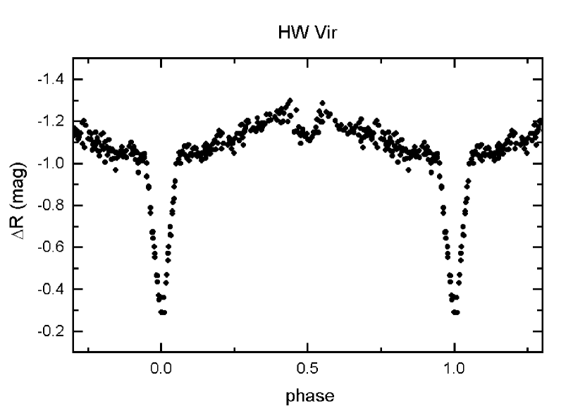
Figure 1: The R-band lightcurve phased with the new ephemeris (E₀=2451670.4125, P=0.116719411 days).

Table 1: Journal of observations

Date	Type	Instr.	Length
2000 ..
May 3/4	photometry (R)	0.28-m SCT	1h
May 5/6	photometry (R)	0.28-m SCT	5h
May 6/7	photometry (R)	0.28-m SCT	5h
May 7/8	photometry (V)	0.28-m SCT	2h
May 25/26	low-res. spec.	0.6-m Schmidt	3h
May 26/27	low-res. spec.	0.6-m Schmidt	3h
May 27/28	low-res. spec.	0.6-m Schmidt	1h
May 30/31	low-res. spec.	0.6-m Schmidt	1h

We obtained digital objective-prism spectra on four nights at the Piszkéstető Station of Konkoly Observatory with the 60/90/180 cm Schmidt-telescope. The detector was a Photometrics AT200 CCD camera (1536x1024 pixels, KAF-1600 chip with UV-coating). The objective prism has a refracting angle of 5^∘ giving 580 Å/mm resolution at H$\gamma$. The observations were unfiltered in order to detect the entire spectral region (approximately between 3800 Å and 9000 Å) limited only by the spectral response of the CCD and the atmospheric transmission. We took 2- to 5-minute exposures, depending on the target brightness and weather conditions. The full log of observations is summarized in Table 1.

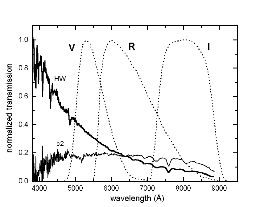
Figure 2: Sample spectra of HW Vir and GSC 5528-0580 (c2) with the VRI passband functions taken from Bessell (1990). Note, that the spectra are scaled arbitrarily and independently for clarity.

The spectral extraction was done with routines developed by the authors. We followed the basic strategy of automatic spectrum detection outlined by Bratsolis et al. (1998). It consists of two main points: i) peak-finding in an integrated profile of the image perpendicular to the dispersion; ii) detection of the end-points of each spectrum. For the wavelength calibration of the extracted spectra, we used two comparison-star spectra with unambiguous spectral features. The first one was Vega (spectral type A0), where the prominent hydrogen Balmer-series lines provided good calibrator data (from H$\alpha$ to H7), while the second one was $\delta$ Vir (spectral type M3). The common features (strong atmospheric telluric lines at 7200 Å, 7600 Å, 8170 Å  identified using the low-resolution spectral atlas of Torres-Dodgen & Weaver 1993), helped adjust the spectra to the same wavelength scale. The eleven well-defined spectral features gave a dispersion curve between 3800 and 8800 Å (with a slight extrapolation at the red end). The residual scatter of calibrating spectral lines is typically about 1 pixel, corresponding to 10–20 Å depending on the spectral region. Finally, we made a relative flux-calibration by dividing the extracted spectra with spectral response function of the instrument (this is a product of the atmospheric transmission and spectral sensitivity function of the CCD chip). It was calibrated with the same spectrum of Vega, knowing its tabulated absolute flux spectrum taken from Gray (1992). Although we observed Vega at the same airmass as HW Vir, a few (2-3) percent uncertainty of the flux levels cannot be excluded due to the possibly changing atmospheric transmission (especially at the blue end of the spectra).

The wavelength and flux-calibrated spectra of HW Vir and two bright stars in the field were used to calculate standard photometric magnitude differences. The used comparisons were c1=GSC 5528-0591, 12$\aas@@fstack{m}$4 and c2=GSC 5528-0580, 12$\aas@@fstack{m}$4. We plot sample spectra for HW Vir and GSC 5528-0580 in Fig. 2, where standard passbands of V, R, and I are also shown (Bessell 1990). By multiplying the calibrated spectra with the filter transmission functions and integrating over wavelength, we determined standard differential V, R, and I magnitudes. Unfortunately, both comparison stars are faint in the blue region, where HW Vir is considerably brighter (see the large scatter below 4500 Å in the spectrum of c2 in Fig. 2), that is why we chose only the VRI bands. The phase diagrams from the obtained 157 points are shown in Fig. 6. The c1$-$c2 differences implied an estimated photometric accuracy of $\pm$0$\aas@@fstack{m}$015 in V and $\pm$0$\aas@@fstack{m}$01 in R and I bands. Times of primary and secondary minima were determined with the same method as applied in CCD photometry, however, these epochs are of lower accuracy due to the meagre phase coverage caused by the relatively long exposures (2-5 min). The eclipse depths are also affected by this phase smearing. All data presented in this paper are available upon request from the first author.

3 Period analysis

The period variation of HW Vir was studied by means of the standard O$-$C technique. For this, we have collected all available times of primary and secondary minimum. Çakirli & Devlen (1999) gave a nearly complete compilation of times of minimum between 1984 and 1997, which had to be updated mainly with the newly published data. These are listed in Table 2. We excluded all of the secondary minima from our analysis, because the depth and sharpness of the primary minimum make the timing more accurate. This was obvious when plotting the whole O$-$C diagram, where the most discordant points were of secondary minima. To be consistent we omitted all secondary minima from the analysis, though some of them were in good agreement with the primary ones. The final sample contains 144 points.

Table 2: Times of minima of HW Vir (HJD$-$2400000). References: (1) ESA 1997, (2) Agerer & Hübscher 1996, (3) Selam et al. 1999, (4) Agerer et al. 1999, (5) Kilkenny et al. 2000, (6) Ogloza et al. 2000, (7) this paper, CCD-R photometry, (8) this paper, objective-prism photometry

Min	Type	Ref.	Min	Type	Ref.	Min	Type	Ref.	Min	Type	Ref.
48500.0801	pri.	1a	50155.5119	pri.	3	50552.4744	pri.	6	50948.3866	pri.	4
49190.24208	pri.	5	50185.39198	pri.	5	50575.46820	pri	5	50955.38977	pri	5
49418.54535	pri.	5	50186.44247	pri	5	50594.3768	pri.	6	50959.24150	pri.	5
49437.57069	pri.	5	50201.38254	pri.	5	50597.29471	pri.	5	51021.21952	pri.	5
49450.64320	pri.	5	50202.43302	pri.	5	50599.27895	pri	5	51183.57618	pri	5
49476.32145	pri	5	50216.67281	pri	5	50600.32943	pri.	5	51190.57932	pri.	5
49480.40663	pri.	5	50218.42364	pri.	5	50604.4147	pri.	6	51216.49105	pri.	5
49485.30883	pri.	5	50222.50883	pri.	5	50631.26003	pri.	5	51236.56678	pri	5
49496.397	pri.	2	50280.28481	pri	5	50883.49067	pri	5	51300.4125	pri.	6
49519.27421	pri	5	50491.4300	pri.	3	50885.47490	pri.	5	51301.3460	pri.	6
49728.55216	pri.	5	50491.4886	sec.	3	50910.45284	pri.	5	51301.4629	pri.	6
49733.57107	pri.	5	50491.5467	pri.	3	50912.55379	pri.	5	51668.4288	pri.	7
49778.6249	pri.	6	50506.48700	pri.	5	50913.50427	pri.	5	51670.3550	sec.	7
49785.6279	pri.	6	50509.52176	pri.	5	50927.3774	pri.	4	51670.4125	pri.	7
49808.5048	pri.	6	50510.57223	pri	5	50927.4938	pri.	6	51670.4717	sec.	7
49833.48294	pri	5	50511.5057	pri.	3	50931.34559	pri.	5	51671.4632	pri.	7
49880.28740	pri.	5	50511.50598	pri.	5	50943.3678	pri.	4	51691.3643	sec.	8
50142.55596	pri.	5	50511.5636	sec.	3	50943.4262	pri.	4	51691.4225	pri.	8
50144.54015	pri	5	50543.72054	pri	5	50943.4843	pri.	4	51692.3561	pri.	8
50147.57490	pri.	5	50547.45557	pri.	5	50946.4024	pri.	4	51695.3905	pri.	8
50155.3946	pri.	3

^a The Hipparcos Epoch Photometry database gives an incorrect doubled period for HW Vir; the listed epoch was determined by us.

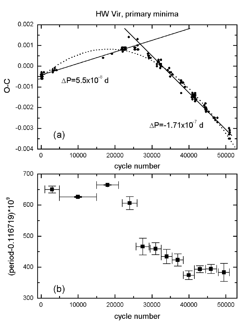
Figure 3: (a): The O$-$C diagram of HW Vir. (b): The “instantaneous period” of HW Vir. The horizontal error bars mark the distance of the neighbouring seasons, while the vertical ones are the standard errors of the linear fits.

We calculated the O$-$C diagram with the following elements taken from Çakirli & Devlen (1999):

Hel. JD${}_{\rm min}=2445730.5565+0.\!\!^{\rm d}1167195820\cdot E$

It is plotted in the top panel of Fig. 3. Our new O$-$C diagram covering almost 52000 cycles (17 years) does not support either periodic solutions with light-time effect or continuous period decrease via smooth and slow mechanisms. One of the simplest and statistically most likely descriptions is assuming two linear branches with a sudden change around cycle number 25000. We fitted two separate models and found a period difference of $(2.25\pm 0.04)\cdot 10^{\rm-7}$ d, a slightly larger value than the $(1.86\pm 0.09)\cdot 10^{\rm-7}$ d determined by Wood & Saffer (1999). We conclude that before 1991 the period was 0$.\!\!^{\rm d}$116719636(1), which changed to 0$.\!\!^{\rm d}$116719411(4).

We have examined the possibility of continuous period decrease. For this reason we fitted a parabola to the O$-$C diagram shown as dotted line in the top panel of Fig. 3. The resulting standard deviation of the residuals is somewhat larger than in the case of two linear fits ($2.1\cdot 10^{\rm-4}$ vs. $1.9\cdot 10^{\rm-4}$). Nevertheless, one could argue that the individual deviations of the O$-$C points from the fitted parabola may be due to some kind of systematic effect, e.g. light-time effect in an undetected binary system. This is one of the usual ways of interpreting cyclic or quasi-cyclic O$-$C diagrams of eclipsing binaries (see, e.g., Borkovits & Hegedüs 1996), thus we have tried to explain the secular period change following this approach. After the parabola subtraction the residuals have a cyclical behaviour, which is the most important condition for assuming a periodic light-time effect solution. However, this possibility has been ruled out with a simple numerical test performed as follows. An artificial O$-$C diagram was calculated with two linear elements divided at the middle of the data (cycle numbers were adjusted to the real case of HW Vir). The O$-$C values were truncated below the expected order of magnitude of accuracy of photoelectric times of minima (0.0001 days). Then we fitted a parabola to the artificial data and the residuals after the subtraction were remarkably similar to the real data. Thus we had to reject the hypothetical light-time effect.

We have also determined the “instantaneous” period from the neighbouring seasons. Its variation can be seen in bottom panel of Fig. 3. We conclude that there are smooth, small-scale, but not strictly repeating changes of the period besides a large jump that happened in less than a year around 1991. These conclusions are substantially very similar to those of Kilkenny et al. (2000), only the time basis is longer by a year.

Accepting two linear parts of the O$-$C diagram, we determined the actual ephemeris, which is very important for effective planning of follow-up observations. It can be used to predict orbital phases provided the period does not change again:

Hel. JD${}_{\rm min}=2451670.4125+0.\!\!^{\rm d}116719411(4)\cdot E$

These elements were used to construct every phase diagram throughout the paper.

What is the reason for the sudden period change? The most common assumption is mass transfer, however in a detached system such as HW Vir it is not expected. Nevertheless, adopting mass transfer to be the responsible cause for period decrease, the primary star had to transfer a mass of about $\sim 3.5\cdot 10^{\rm-5}$ M_⊙. But, as was noted by Wood & Saffer (1999), it is unclear why such an event would occur. One could consider outer accretion, e.g., engulfing a planet-size body. The required mass (double the amount above to get the same change of the mass-ratio) is only in the range of tens of Earth masses, however, since we have no additional data, this is only rough speculation.

4 The components of HW Vir

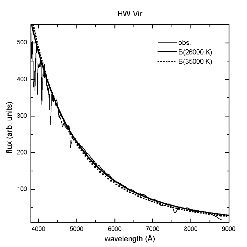
Figure 4: The observed spectrum at $\phi=0.93$ with two blackbody fits.

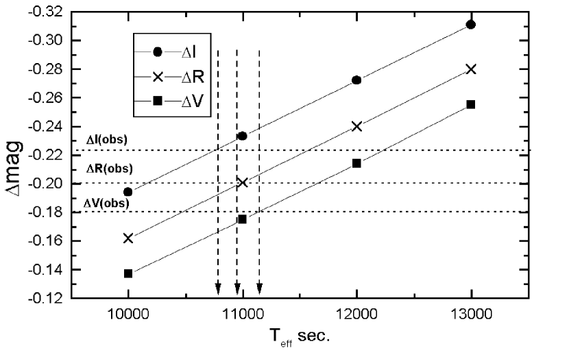
Figure 5: A multiband estimate for the disk-averaged temperature of the illuminated surface of the secondary component. The “obs” subscript and the dotted lines correspond to the observed amount of the reflection effect (i.e. the magnitude difference of the V, R, and I band lightcurves between $\phi=0.58$ and $\phi=0.93$). The model lines were calculated with blackbody approximation (T_eff(pri.)=26000 K).

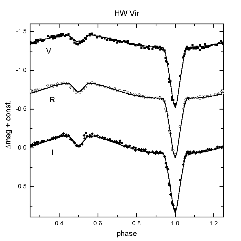
Figure 6: Lightcurve models for HW Vir

Beside revealing the current period variation of HW Vir, our observations addressed the spectroscopic detection of the cool secondary component. One possible detection of this faint star was presented by Wood & Saffer (1999), who found evidence for weak additional H$\alpha$ absorption lines around the maximal reflection effect (at $\phi$=0.58). They attributed these lines to irradiation of the face of the secondary star closest to the sdB star. However, there has been no identification of the secondary during the primary minimum, when the system is seen from the direction of the cooler hemisphere. Our spectral coverage is only slightly extended toward the infrared than that of Wood & Saffer (1999), which has been the “reddest” spectroscopy so far (up to 8667 Å). Since the eclipse depth of the primary minimum is the same in all three bands (0$\aas@@fstack{m}$72), we conclude that we have not detected the red continuum of the secondary.

The most striking feature of the lightcurve is the prominent reflection effect. As has been noted by Włodarczyk & Olszewski (1994), the effect gets stronger with the increasing wavelength (they obtained 0$\aas@@fstack{m}$17 in B, 0$\aas@@fstack{m}$18 in V and 0$\aas@@fstack{m}$21 in R). We have also determined the amount of reflection as the magnitude difference between $\phi$=0.58 and $\phi$=0.93. We obtained 0$\aas@@fstack{m}$18 in V, 0$\aas@@fstack{m}$20 in R and 0$\aas@@fstack{m}$22 in I the first two values being in good agreement with those of Włodarczyk & Olszewski (1994). They were used to estimate the mean heating of the secondary.

In what follows we outline a simple consideration on the reflection effect based on blackbody approximation. We have to stress that we did not want to present a new Wilson–Devinney-type lightcurve solution, but we use their constraints on the components. All of the published lightcurve models are in good agreement concerning the radii for both components, approximately the same value around 0.2 R_⊙. The presented values range from 0.18 R_⊙ to 0.22 R_⊙, thus a $\sim$10% uncertainty can be roughly assumed. Fortunately, all models in the literature agree in one aspect: both stars have essentially the same radius, which is the most important assumption in what follows. The most significant difference is related with the temperature of the primary: the estimates are between 26000 K (Włodarczyk & Olszewsi, 1994) and 36000 K (Çakirli & Devlen 1999). To obtain an independent estimate we fitted the continuum observed just before the primary minimum ($\phi=0.93$) with a Planck function. In the chosen phase the illuminated secondary hemisphere is hidden and the primary totally outshines the secondary. This can be seen in Fig. 4, where two Planck functions are shown with the observed spectrum. Obviously, either 26000 K or 35000 K fits almost equally well the observed spectrum. Keeping in mind the possible few percent uncertainty of the flux calibration, we can claim that our data give only limits on the primary’s temperature. We can solidly exlude 25000 K and 40000 K for the lower and upper limits, respectively (the hotter limit is less determined, as suggested from the lightcurve modelling discussed below).

We have synthesized combined spectra of primary+irradiated secondary by co-adding two different blackbody flux distributions with the same weighting factors (i.e. we assumed equal surfaces of the components). First we fixed the primary’s temperature at 26000 K and varied the second blackbody’s temperature between 10000 and 13000 K. Then we calculated the standard V, R, and I magnitude differences between the single blackbody and combined flux distribution. We plot these magnitude differences versus the secondary temperatures in Fig. 5. The observed strengths of the reflection effect result in a disk-averaged temperature of 11000$\pm$200 K for the brighter hemisphere of the secondary. Repeating this procedure with a fixed primary temperature of 35000 K we got 13300$\pm$200 K for the secondary. These values give a constraint on the albedo of the secondary. Accepting approximate geometric parameters of the system (two stars with radii of 0.2 R_⊙ at a distance about 0.9 R_⊙), a perfect blackbody and flat secondary would be heated to 14500 K (12500 K) by a 35000 K (26000 K) hot primary. The fact that a limb-darkened average radiation of the irradiated secondary can be approximated by a blackbody close to the ideal case, suggests an albedo near unity.

We have calculated synthetic binary lightcurves using the BINARY MAKER package by Bradstreet (1993). Let us emphasize again that we did not want to present a new lightcurve solution, because our data are not well suited for this purpose. For instance, the eclipse depth of the primary minimum is decreased by 0$\aas@@fstack{m}$02–0$\aas@@fstack{m}$03 to 0$\aas@@fstack{m}$72 due to the relatively long exposures applied during the faintest state (4-5 minutes), while photometric observations with higher time-resolution yield 0$\aas@@fstack{m}$75. Therefore, our model should be considered as an approximate one. We adopted the following parameters of the components for calculating the model lightcurves plotted in Fig. 6: q=0.3; i=80$.\!\!^{\circ}$2; T₁=35000 K; T₂=3250 K (assumed); r₁=0.2; r₂=0.2; gravity darkening 1 and 0.32; limb-darkening (1) 0.3, 0.25, 0.20 (VRI); limb-darkening (2) 0.0, 1.0, 0.8 (VRI); albedo (1) 1, 1, 1 (VRI); albedo (2) 0.7, 0.7, 0.8 (VRI). We largely followed Kilkenny et al. (1998) in choosing various parameters, as they used the same package. The assumed binary parameters are the same as in the previous studies. It is interesting that we did not have to choose unity albedo, but slightly smaller values giving acceptable curves. Generally, the models are in good agreement with the observed lightcurve shapes, only the calculated secondary minima are shallower by about 0$\aas@@fstack{m}$01 than the observed ones. They can be made deeper by increasing the primary temperature up to 40000-44000 K, but this is in contradiction with the wide-band flux distribution.

The temperature ambiguity recalls the question of distance to HW Vir. The Hipparcos parallax is 1.8$\pm$1.9 mas (ESA 1997), where the large uncertainty is most probably due to the faintness of the star. Furthermore, the Hipparcos parallax error on HW Vir is only 1-$\sigma$, thus assuming normal distribution it means that there is 16% chance for the parallax being larger than 3.7 mas and 2.5% for 5.6 mas. Briefly, the Hipparcos parallax is not significant, essentially unknown. The 95% significance limit would imply a highest parallax limit of 1.8 mas+2$\cdot\sigma=$5.6 mas corresponding to a minimal distance of 179 pc. This lies close to the the larger range of published photometric and/or spectroscopic distances suggesting the close proximity (e.g. 42 pc) to be unlikely. Keeping in mind the quoted uncertainties, the presently available trigonometric data yield only very rough order of magnitude estimates.

5 Summary

The new results presented in this paper can be summarized as follows:

1. New photometric observations are presented revealing the recent period change of HW Vir. The O$-$C diagram covering 17 years does not support earlier suggestions of a possible light-time effect, but can be very well described by two linear branches. There are also additional smooth period changes.

2. Low-resolution objective-prism spectra were obtained and standard VRI photometry was done by convolving the calibrated spectra with the filter transmission functions. Our I-band lightcurve is the first in the literature. We have tried to detect spectral features that can be associated with the cool secondary component (e.g. variations in the infrared continuum), but this attempt failed. The depth of the primary minimum is the same in all three bands suggesting that the secondary is totally invisible even in the I band.

3. We present a simple estimate for the mean effective temperature of the illuminated hemisphere of the secondary based on the V, R, and I magnitude of the reflection effect. Their values (0$\aas@@fstack{m}$18, 0$\aas@@fstack{m}$20 and 0$\aas@@fstack{m}$22) give a 13300$\pm$200 K or 11000$\pm$200 K temperature depending on the adopted primary temperature, which implies a near unity albedo for the cool component. This is also supported by an approximate lightcurve model.

- (1) Agerer F., Hübscher J. 1996, IBVS No. 4382
- (2) Agerer F., Dahm M., Hübscher J. 1999, IBVS No. 4712
- (3) Bessell M.S. 1990, PASP 102, 1181
- (4) Borkovits T., Hegedüs T. 1996, A&AS 120, 63
- (5) Bradstreet D.H. 1993, BINARY MAKER 2.0, Contact Software
- (6) Bratsolis E., Bellas-Velidis I., Kontizas E. et al. 1998, A&AS 133, 293
- (7) Çakirli Ö., Devlen A. 1999, A&AS 136, 27
- (8) Carnochan D.J., Wilson R. 1983, MNRAS 202, 317
- (9) ESA 1997, The Hipparcos and Tycho Catalogues, ESA SP-1200
- (10) Gray D.F. 1992, Observations and analysis of stellar photospheres, Cambridge University Press, New York
- (11) Hilditch R.W., Harries T.J., Hill G. 1996, MNRAS 279, 1380
- (12) Kilkenny D., Marang F., Menzies J.W. 1994, MNRAS 267, 535
- (13) Kilkenny D., O’Donoghue D., Koen C. at al. 1998, MNRAS 296, 329
- (14) Kilkenny D., Keuris S., Marang F. et al. 2000, Observatory 120, 48
- (15) Menzies J.W. 1986, Ann. Rep. S. Afr. Astron. Obs. 1985, p.20
- (16) Menzies J.W., Marang F. 1986, IAU Symp. 118, Instrumentation and Research Programs for Small Telescopes, Reidel, Dordrecht, p.305
- (17) Ogloza W., Drózdz M., Zola S. 2000, IBVS No. 4877
- (18) Selam S.O., Gural B., Muyesseroglu Z. 1999, IBVS No. 4670
- (19) Torres-Dodgen A.V., Weaver W.B. 1993, PASP 105, 693
- (20) Włodarczyk K., Olszewski P. 1994, AcA 44, 407
- (21) Wood J.H., Zhang E-H., Robinson E.L. 1993, MNRAS 261, 103
- (22) Wood J.H., Saffer R. 1999, MNRAS 305, 820