The Cosmic Electron Background in Low Energy IACTs. Effect of the Geomagnetic Field
Abstract
A new generation of low threshold Imaging Atmospheric Cherenkov Telescopes (IACTs) may reach -ray energies about 10 GeV with high sensitivities and very large collection areas. At these low energies cosmic electrons significantly contribute to the telescope background and are in principle indistinguishable from -rays. In this paper we estimate the electron background expected for two configurations of the low energy IACT MAGIC. We discuss in particular the reduction of the background caused by the geomagnetic field at different locations on the Earth’s surface.
PACS: 95.55.Ka
Keywords: -rays, atmospheric Cherenkov detectors,
sensitivity, electron background, geomagnetic, GeV-TeV energies.
Accepted for publication in Astroparticle Physics.
1 Introduction
A number of low energy threshold Imaging Atmospheric Cherenkov Telescopes are under design or construction and will cover the -ray region from 10 GeV to 10 TeV. Ground-based instruments [1] provide high sensitivities and huge collections areas of the order of 105 m2, i.e. orders of magnitude higher than those achievable by satellite experiments in the same energy range like GLAST [2].
In this paper we shall concentrate on the IACT MAGIC [3, 4] since this project aims at the lowest energy threshold. The MAGIC collaboration is currently building a 17 meter diameter telescope equipped with a 600 PMT pixel camera (MAGIC phase I) which will reach an energy threshold of 30 GeV [4] (defined as the peak in the raw differential rate, i.e., before any selection cuts). In its second phase the camera will be equipped with high quantum efficiency hybrid PMTs (HPD) that will lower the energy threshold down to 10 GeV. A third phase may use a camera with Avalanche PhotoDiodes (APDs) of even higher efficiency, but we will not consider this for our studies.
IACTs have to deal with a background of electron- and hadron-initiated atmospheric showers. At very low energies below 50 GeV hadrons rarely generate enough Cherenkov light to trigger the telescope. According to [4, 5] its contribution to the background is negligible below 30 GeV. In turn cosmic electrons will give rise to showers which are practically indistinguishable from -induced ones and thus can not be eliminated using traditional -hadron discrimination methods. They are isotropic and can be suppressed by means of an improved angular resolution when the telescope searches for point sources, but they constitute an irreducible background in extended source searches and diffuse gamma flux estimations.
The purpose of this paper is to estimate the fluxes and detection rates of cosmic electrons expected in the new generation IACT MAGIC in its phases I and II. In particular we shall carefully consider the effect of the geomagnetic field on the electron background observed at ground level.
2 Geomagnetic Field and Rigidity Cutoffs
The Geomagnetic Field (GF) is a combination of several magnetic fields produced by different sources. More than 90% of the field is generated inside the Earth and is known as “main field” or “internal field”. The main field is usually described as a dipole (as in the original work of Störmer [6]) or more precisely as a high order harmonic expansion whose coefficients are based on experimental observations and updated every few years, the so-called International Geomagnetic Reference Field (IGRF).
The solar wind interacts with the Earth’s field and its effect is described by an external field. The currents induced in the magnetosphere and ionosphere may create magnetic fields as large of 10% of the main field and are variable on a much shorter time scale. Magnetohydrodynamic models are called for in order to describe the whole GF, such as Tsyganenko model [7] or the Integrated Space Weather Prediction Model (ISM) [8, 9]. The GF bends the cosmic ray trajectories preventing low rigidity particles from reaching the Earth’s surface. (The rigitidy of a particle is defined as pc/ze, where c is the speed of light, p is the momentum and ze is the charge of the particle). The minimum allowed rigidity is know as rigidity cutoff. In the case of a dipole GF the rigidity cutoffs can be calculated analytically [6]. In this paper we will draw mainly on an expression for the rigidity cutoff () given by Cooke[10] which is based on a dipole approximated to the IGRF1980:
| (1) |
where is the magnetic latitude, is the zenith angle, is the azimuth angle measured clockwise from the magnetic north and is the distance from the dipole center (in Earth radius units). Analytical procedures always underestimate due to the effect of the Earth shadow effect. A subset of the trajectories intersect the Earth and are physically impossible. This results in a region of rigidities some of which are allowed and some forbidden, usually referred to as penumbra. The penumbra can be studied by ways of numerical procedures of backtracking [11, 12]. The highest forbidden energy, so-called upper rigidity cutoff, is 5–30% higher than [13, 14].
values in the zenith direction according to equation 1 are tabulated in table 1 for some geomagnetic latitudes. MAGIC will actually be built very close to a geomagnetic latitude of 30∘N. Included in the table are the extreme cases of the magnetic pole (90∘ magnetic latitude), for which all trajectories are allowed, and the magnetic equator (0∘ magnetic latitude) for which the cutoff energy reaches a maximum.
3 The Electron Background
Electron detection rates
In the following we will make the assumption that electron-initiated showers behave exactly like gamma-initiated ones.
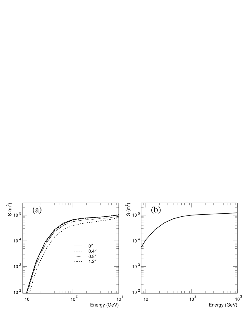
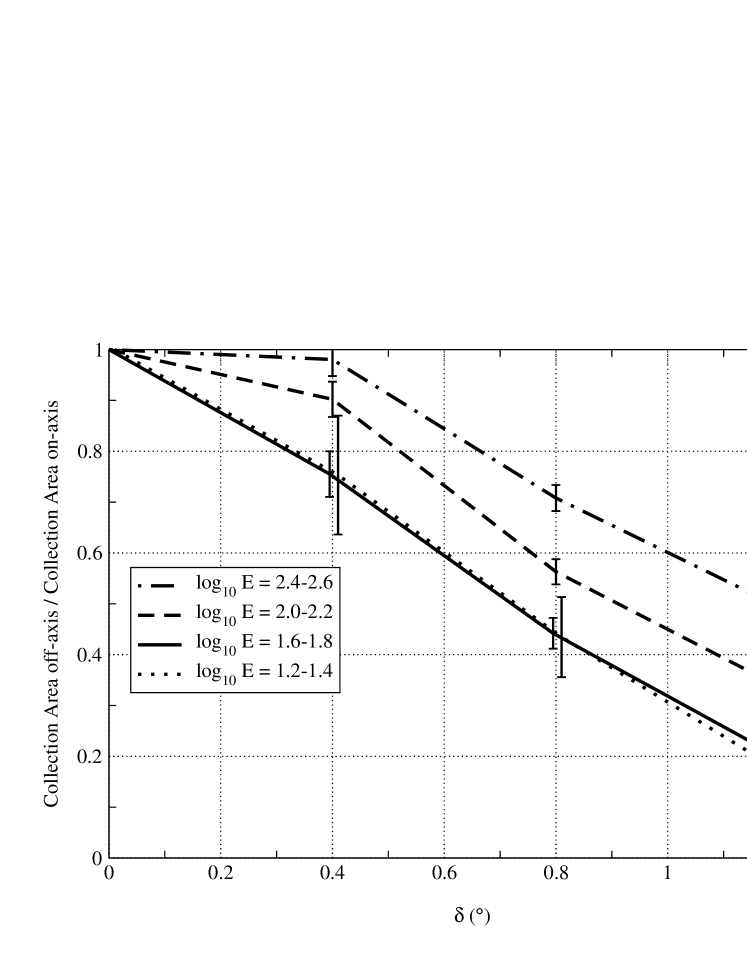
Figure 1 shows the MAGIC raw collection area (i.e. with no selection cuts) at zenith for gamma primaries in the case of the PMT camera (MAGIC phase I, figure 1a) and of the HPD camera (MAGIC phase II, figure 1b). The collection area for primaries was calculated using a Monte Carlo simulation of the shower development in the atmosphere and the response of the detector to the Cherenkov light produced in the shower (see [4, 5] for details). A trigger condition of four next-neighbour pixels with at least 7 photoelectrons in a trigger region of 0.8∘ radius was adopted. Electrons arrive isotropically in the camera, so the shower axis was generated parallel to the telescope pointing direction (“on-axis”), but also with a certain angle with respect to this direction (“off-axis”) in order to characterize all possible incident directions. In particular =0∘, 0.4∘, 0.8∘ and 1.2∘ were simulated. Figure 1 shows the collection area () in MAGIC phase I for these directions. The uncertainties in are always below 10%. Figure 2 shows as a function of . has been normalized to the on-axis collection area () in order to show how the trigger efficiency decreases with . The dependence of / on has been plotted for four different energies. For phase II no simulation of off-axis showers was available, hence we assume in our calculations that the fractions for phase I hold valid for phase II and we can use them to obtain the collection areas off-axis out of the collection areas on-axis.
We can use the raw collection areas along with the electron energy spectrum displayed in figure 3 (taken from [15]) in order to estimate the raw rate of electron triggers in MAGIC. In doing so we assume that electrons arrive isotropically with 1.5∘ and that can be calculated from the correlations in figure 2. Figure 4 shows the electron raw differential rate and integral rate at zenith as a function of electron primary energy. The uncertainties in the rates are basically determined by the uncertainties in the primary electron spectrum which range from 40% at energies around 10 GeV down to 35% around 1 TeV.
The rate estimated for phase I (2.81.2 Hz) is significantly lower than the rate quoted in [4] (9 Hz). This stems from two reasons. To begin with, we have correctly taken into account the decrease of collection area as a function of off-axis angle whilst [4] assumed that the collection area off-axis could be approximated by the on-axis collection area. Besides the authors of [4] did actually not quote the expected electron rate but rather an upper limit to this rate based on the upper limit to the electron differential spectrum [16]. The electron rates obtained represent a few percent of the hadron rate expected for both phases I and II [4, 5].
Let us consider now the effect of the geomagnetic rigidity cutoff on the electron rates. In table 2 we tabulate the electron fluxes and rates one expectes at different locations on Earth as listed in table 1. Also shown is the fraction of the polar rate (rate at the magnetic pole). The polar rate is equal to the rate that we would obtain neglecting the rigidity cutoff. The table displays the rates for both phases of MAGIC pointing to the zenith position. The errors in the rates mostly come from the uncertainties in the primary electron flux. It must be emphasized that the fractions of the polar rate suffer from no uncertainty since the errors in both polar and reduced rates are correlated. For MAGIC phase I the effect of is small for almost all the locations under consideration. Only at the magnetic equator do we observe a 25% reduction in the rate. In contrast for MAGIC phase II one expects a noticeable reduction in the rate, especially for low magnetic latitudes and as high as a factor of 2 at the geomagnetic equator.
In all previous calculations we have assumed that there is an abrupt cut in the electron energy spectrum at the position of the rigidity cutoff, that is, we have ignored the penumbra. We may obtain an upper limit to the effect of the penumbra in the electron rate by assuming that all trajectories inside this energy region are forbidden and that the upper rigidity cutoff is always 25% higher than the rigidity cutoff. In this extreme case we obtain further reductions in the electron rate of at most 20%.
Telescope sensitivity
We consider now the limits that the electron background pose to the detector sensitivity. Contrary to hadron showers, electron showers behave exactly like showers. Therefore they cannot be rejected using separation procedures based on the shower image characteristics. For point source searches, electrons which do not come from the source direction may be rejected within the angular resolution capabilities of the detector. But for diffuse or extended sources, no rejection is possible. (By “diffuse source” we understand a source which emits homogenously inside our camera’s field of view, while by “extended source” we refer to any non-point source).
The sensitivity of an IACT is generally defined as the -ray flux necessary to produce a 5 signal in 50 hours of observation. For simplicity we suppose that the -ray source has the same spectral index as the electron background. The sensitivity for diffuse sources at 5, 10 and 50 GeV for different geomagnetic locations can be found in table 3. A 5% improvement is found when going from the magnetic pole to the magnetic equator in MAGIC phase I. The improvement in phase II is more considerable. The sensitivity at the equator increases by 13% at 10 GeV and by 45% at 5 GeV.
In the case of point sources we can reject electron showers which do not come from the source direction. By using the standard Hillas analysis methods (in particular cutting at ALPHA parameter greater than 15∘) we can reduce the number of electrons by a factor of 6, while keeping 70% of the gammas (see page 159 of reference [4]. Taking into account the orientation of the shower image (“head-tail”), it may be possible to reject 50% of the remaining electrons). The polar sensitivity for point source detection in MAGIC phase I is found to be = 2.410-10 cm-2s-1. The proportionality factor between this sensitivity and the corresponding diffuse source sensitivity can be applied to all the other sensitivities in table 3 to obtain the point-source sensitivities at 5 and 10 GeV, and, with good approximation, also at 50 GeV. The effect of the geomagnetic field will thus be the same for diffuse and point sources.
Most of the extended sources constitute intermediate cases between the aforementioned point and diffuse sources. In consequence the telescope sensitivity for a general extended source will be determined by its actual angular size, but will always have a value between the sensitivities calculated for diffuse and point sources.
The hadronic background is strongly reduced at energies around 10 GeV and the electron sensitivity limits which we have calculated are in the order of or above the limit imposed by the hadronic background [4]. Therefore any accurate measurement will have to take into account the presence of the electron background and the effect of the geomagnetic field.
Dependence on zenith angle
Until now we have restricted our analysis to the zenith position of the IACTs. Let us try to predict the geomagnetic cutoff effect at other zenith angles. The dependence of the electron rigidity cutoff on zenith angle for a number of azimuth angles and geomagnetic latitudes according to equation (1) is given by figure 5. Whereas the cutoff does not vary strongly with the zenith angle for geomagnetic latitudes above 30∘ (at most a 50% increase from 0 to 90∘ zenith angle in all azimuth directions), it rises by as much as a factor of 3 in the geomagnetic equator. A given IACT exhibits approximately the same collection area and energy threshold for all zenith angles below 30∘. Hence let us apply the zenith collection areas shown in figure 1 to all zenith angles below 30∘. The maximal reduction in electron rate takes place in the magnetic equator when the telescope points to the east. The maximal enhancement happens also in the equator when the telescope points to the west. We have tabulated the rates expected for MAGIC phase II in table 4 at geomagnetic latitudes 0∘ and 30∘ in the west and east directions. The maximal rate reduction is 30% whilst the maximal enhancement is 20%. MAGIC phase II sensitivity will thus improve slightly when pointing to the west and get slightly worse when pointing to the east. The effect of the zenith angle is expected to be smaller in the case of MAGIC phase I.
Conversely the IACT energy threshold increases fast with zenith angle above 30∘ (see for example [17, 18, 19]). At a zenith angle of 60∘ the energy threshold is already roughly one order of magnitude higher than the threshold close to the zenith. Because the cosmic electron spectrum falls with primary energy faster than that of the cosmic ray background or than those of most of the predicted -ray sources we can expect the electron background to be less and less significant as we move to higher zenith angles. In addition the effect of the geomagnetic cutoff will decrease with zenith angle since does not grow as fast as the telescope threshold energy. Electrons triggering the telescope are thus never below .
4 Valididy of the Geomagnetic Model
Equation (1) is based on a dipole field. Hence we may consider to improve our calculations by applying a more realistic main field such as the IGRF. Nevertheless because the dipole in equation (1) was approximated to the IGRF1980 value, we do not expect our results to differ considerably from the real values. It must be emphasized that no analytical solution for the rigidity cutoff is possible by using a field model more complex than a dipole field.
Besides, we have always neglected in our calculations the effect of the external geomagnetic field described in section 2. As already mentioned, under normal conditions this field contributes up to 10% of the global field intensity. The external field, however, is asymmetric due to the interaction of the Earth with the solar wind, which gives rise to a long tail extending to the direction almost opposite to that of the Sun (actually in a direction perpendicular to the solar wind front, but for simplicity we assume that it extends in a direction opposite to the Sun). This introduces an asymmetry in the electron arrival direction, since electrons going through the tail are more likely to be deflected than electrons coming from the direction of the Sun. In other words, we expect the rigidity cutoff to grow in the direction opposite to the Sun. For a given arrival direction this is a daily effect. As a consequence we expect the minimum electron rate to be reached at midnight in the zenith direction. Since IACTs operate only at night, the electron rate will on the whole be further reduced by this effect.
A detailed study would necessitate taking into account the fast variations of the external field produced during periods of increased solar activity. In general these periods profoundly complicate the calculation of rigidity cutoffs and background electron rates. Careful planning of IACT observations for special studies of extended sources or the diffuse gamma background will be necessary during these periods.
5 Conclusions
We have estimated the electron background expected in both phases of the low-energy-threshold IACT MAGIC at different geomagnetic latitudes. The raw electron rate expected for MAGIC phase I is approximately 3 Hz in the zenith direction at the magnetic pole and drops to 2.5 Hz at the magnetic equator. For MAGIC phase II these rates are correspondingly 20 and 10 Hz. The reduction with decreasing magnetic latitude reflects the fact that the electron rigidity cutoff is minimal at high geomagnetic latitudes and maximal at the equator. The sensitivity is also improved when going to lower latitudes by as much as 50% for at the equator. The detection rate decreases for some azimuth angles reaching a minimum when the telescope points to the west and increase for other angles peaking in the east direction. The electron background is expected to be very much reduced in high zenith angle observations.
The conclusion can be drawn that any estimate of the -ray flux of an extended source or of the isotropic -ray flux will have to take into account the geomagnetic location of the IACT as well as the specific direction in which the instrument is pointing, especially for observations in which the zenith angles are less than 30∘.
6 Acknowledgments
The authors are deeply grateful to many members of the MAGIC Telescope collaboration for their assistance and interesting comments. We wish to thank especially R. Mirzoyan and E. Lorenz for their useful remarks and suggestions. One of the authors (J.C.) gratefully acknowledge discussions with S. Orloff.
References
- [1] Lorenz E. et al.; Hofmann W. et al.; Krennrich et al.; Mori M. et al.; all contributions in Proc. Towards a Major Atmospheric Cherenkov Detector VI, in press.
- [2] Kniffen D. et al., 1999, Proc. Towards a Major Atmospheric Cherenkov Detector VI, in press.
- [3] Bradbury S. M. et al., 1995, Proc. Towards a Major Atmospheric Cherenkov Detector IV, ed. M. Cresti, p. 277.
- [4] Barrio J. A. et al., 1998, The MAGIC proposal, Max Planck Institut für Physik Munich report MPI-PhE/98-5.
- [5] González J. C., PhD Thesis, Universidad Complutense de Madrid (2000), in preparation.
- [6] Störmer C., Astrophys. 1 (1930) 237.
- [7] Tsyganenko N. A., Planet. Space. Sci. 37 (1989) 5.
- [8] Erickson G. M. et al., J. Geophys. Res. 96 (1991) 1633.
- [9] Lambour R. L., PhD Thesis, Rice University (1994).
- [10] Cooke D. J., Phys. Rev. Lett. 51 no. 4 (1983) 320.
- [11] Shea M. A. and Smart D. F., J. Geophys. Res. 72 no. 7 (1967) 2021.
- [12] Flückiger E. O. et al., Proc. 22nd ICRC Dublin 3 (1991) 648.
- [13] Shea M. A. and Smart D. F., J. Geophys. Res. 70 no. 17 (1965) 4117.
- [14] Lipari P. and Stanev T., Proc. 24th ICRC Rome 1 (1995) 516.
- [15] Wiebel-Sooth B., PhD Thesis, Wuppertal University (1998).
- [16] Lorenz E., private communication.
- [17] Krennrich F. et al., Ap. J. 511 (1999) 149.
- [18] Ibarra A. et al., 1999, Proc. Towards a Major Atmospheric Cherenkov Detector VI, in press.
- [19] Konopelko A. et al., 1999, Proc. Towards a Major Atmospheric Cherenkov Detector VI, in press.
| Magnetic latitude | Rigidity cutoff (GV) |
|---|---|
| Magnetic pole 90∘ | 0. |
| 75∘ | 0.1 |
| 60∘ | 0.9 |
| 45∘ | 3.7 |
| 30∘ | 7.3 |
| 15∘ | 12.9 |
| Magnetic equator 0∘ | 14.9 |
| Magnetic | Rate phase I | Fraction | Rate phase II | Fraction |
| latitude | (Hz) | polar rate | (Hz) | polar rate |
| Mag. pole | 2.81.2 | 1.00 | 218 | 1.00 |
| 75∘ | 2.81.2 | 1.00 | 218 | 1.00 |
| 60∘ | 2.71.2 | 0.96 | 208 | 0.95 |
| 45∘ | 2.71.2 | 0.96 | 208 | 0.95 |
| 30∘ | 2.71.2 | 0.96 | 176 | 0.80 |
| 15∘ | 2.51.2 | 0.89 | 115 | 0.52 |
| Mag. equator | 2.41.0 | 0.77 | 104 | 0.48 |
| Magn. | ||||
| lat. | (cm-2 s-1 sr-1) | (cm-2 s-1 sr-1) | (cm-2 s-1 sr-1) | |
| Phase I | 90∘ | 4.110-6 | 1.010-6 | 4.710-8 |
| 30∘ | 4.110-6 | 1.010-6 | ||
| 15∘ | 4.110-6 | 1.010-6 | ||
| 0∘ | 3.910-6 | 9.510-7 | ||
| Phase II | 90∘ | 1.610-6 | 4.410-7 | 3.510-8 |
| 30∘ | 1.510-6 | 4.410-7 | ||
| 15∘ | 1.210-6 | 4.410-7 | ||
| 0∘ | 1.110-6 | 3.910-7 |
| Location | Azimuth | 0∘ ZA | 30∘ ZA |
|---|---|---|---|
| Lat. 30∘ | East | 176 | 145 |
| West | 186 | ||
| Lat. 0∘ | East | 104 | 73 |
| West | 125 |