Probing the gravitational potential of a nearby lensing cluster Abell~2104

Abstract

The cluster Abell~2104 is one of the lowest redshift clusters ($z=0.153$) known to have a gravitational lensing arc. We present detailed analysis of the cluster properties such as the gravitational potential using the X-ray data from ROSAT (HRI) and ASCA, as well as optical imaging and spectroscopic data from the CFHT. The cluster is highly luminous in the X-ray with a bolometric luminosity of $L_{x}\sim 3\times 10^{45}$ ergs s^-1 and a high gas temperature of $\sim 10.4$ keV. The X-ray emission extending out to at least a radius of 1.46 Mpc, displays significant substructure. The total mass deduced from the X-ray data under the assumption of hydrostatic equilibrium and isothermal gas, is found to be $M_{tot}(r<1.46\mathrm{Mpc})\sim(8.0\pm 0.8)\times 10^{14}M_{\sun}$. The gas fraction within a radius of 1.46 Mpc is $\sim 5-10$%. The cluster galaxy velocity distribution has a dispersion of $1200\pm 200$ km s^-1 with no obvious evidence for substructure. The total mass within 1.46 Mpc, deduced from Jean’s equation using the observed galaxy number density distribution and velocity dispersion, is found to be $\sim 6.8\times 10^{14}M_{\sun}$ to $\sim 2.6\times 10^{15}M_{\sun}$ marginally consistent with the X-ray deduced total mass.

1 Introduction

Clusters of galaxies are the largest bound systems in the Universe, and as such they are the largest objects where detailed studies of their gravitational potential are possible. Given their large sizes, 3 to 6 Mpc in extent, they are also thought to be representative of the Universe in terms of the baryonic fraction which is directly related to the density of the universe and the predictions of the Big Bang nucleosynthesis theory. Studies so far have found that the baryonic fractions in clusters favour a low matter density universe given the predictions of baryon densities given by the nucleosynthesis theory (e.g. White et al. 1993). Recently, detailed and independent estimates of cluster total mass distributions have become available; the mass–tracers used and the observational techniques employed can be summarised as follows:

• Cluster Galaxies : these have a long tradition of providing mass estimates via application of the Virial Theorem to the observed dispersion in their radial velocities. The method rests upon the assumption that the galaxies are in dynamical equilibrium.

• Hot Intracluster Gas : as well as being an important mass component of clusters, its X-ray emission provides an ideal tracer – through the hydrostatic equation – of the total underlying mass. The assumption that the gas is in hydrostatic equilibrium with the cluster’s gravitational potential is thought to be reasonably secure for the central few Mpc (Evrard et al. 1996 and Schindler 1996) and the gas density and temperature profiles required to solve the hydrostatic equation are readily available from the X-ray data.

• Gravitational Lensing : here the lensing action of the cluster on background sources, as revealed in deep high resolution imagery (Tyson et al. 1990; Fort & Mellier 1994 and references there in), is used to provide a direct measure of the shape and depth of the cluster potential and hence the projected mass distribution (Kaiser & Squires 1993, Broadhurst et al. 1995 etc.). Unlike the first 2 methods, this approach is not reliant upon assumptions of hydrostatic or dynamical equilibrium.

For detailed studies in the X-ray and optical, we need a nearby cluster, though gravitational lensing effects are diminished for low redshift clusters. An ideal cluster for this kind of detailed and independent estimates of mass distributions, would be one of the lowest redshift clusters with obvious lensing effects such as a giant arc. In this paper, we will analyse the X-ray and optical data for one of the nearby lensing clusters.

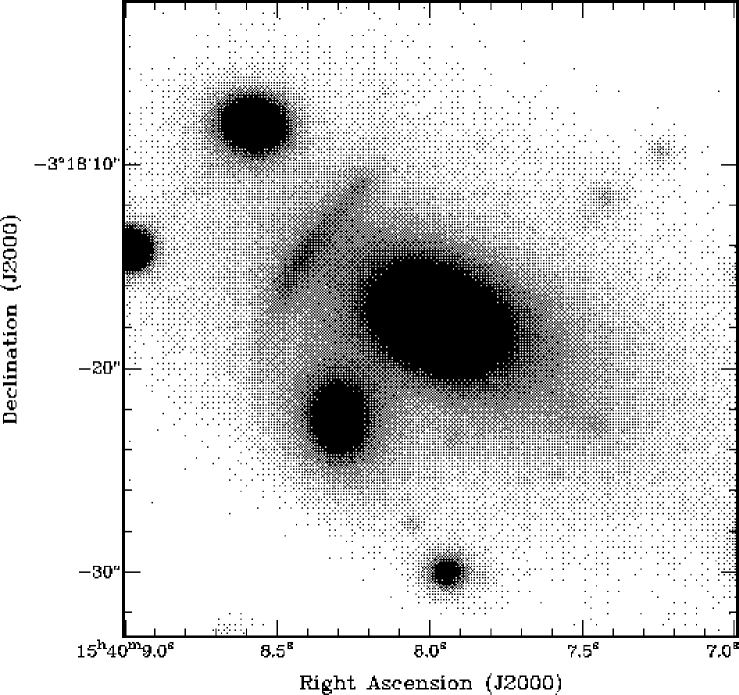
Abell~2104 is a rich cluster (richness class 2) at a redshift of 0.155 (Allen et al. 1992). It was found to have a high X-ray luminosity from the ROSAT all-sky survey data (Pierre et al. 1994). Subsequent optical followup observations with the CFHT revealed an arc embedded in the halo of the central cD galaxy $7\aas@@fstack{\prime\prime}2$ away from the centre (Pierre et al. 1994). The arc spans $10\arcsec$ in length and it is amongst the reddest known arcs. Fig. 2 shows a close up picture of the arc. Given the small arc radius, it is important to have a high resolution X-ray observation with an instrument such as the ROSAT/HRI to probe the gravitational potential within the arc radius.

The optical data including photometry and spectroscopy will be analysed in Sec. 2. The spatial and spectroscopic analysis of the X-ray data from ROSAT and ASCA will be given in Sec. 3. The independent mass estimates using different methods as well as a comparisons will be given Sec. 4.

Throughout the paper we adopt a cosmological model with $H_{0}=50$ km s^-1Mpc^-1, $\Omega_{0}=1$ and $\Lambda_{0}=0$. Celestial coordinates are in J2000.

2 Optical data

2.1 Observations

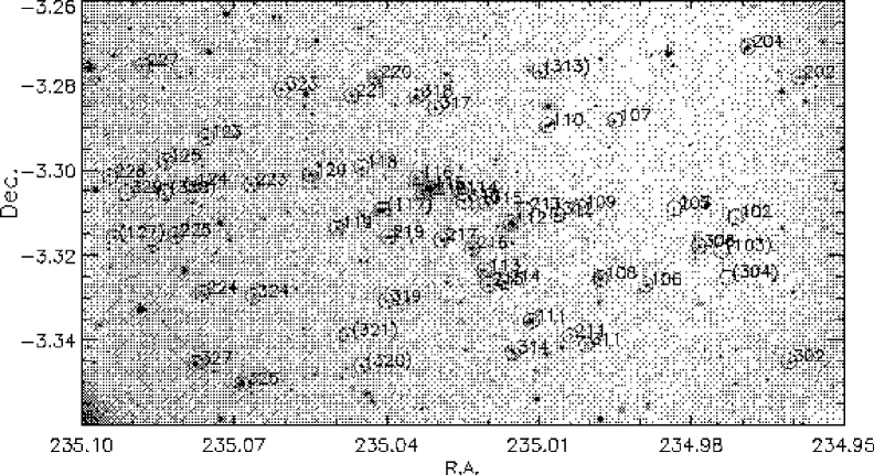
The data were collected in 4 nights at the 3.6 m CFHT Telescope in May 1993. Two 10 minutes exposures in B band and two 15 minutes exposures in R band were obtained. Exposures of 30 to 55 minutes per spectroscopic mask was obtained for 3 separate masks, each containing about 30 slits (Fig. 3). The focal reducer MOS/SIS together with CCD Lick2 ($2048\times 2048$ pixels of 15 $\mu$m) were used during the run. This CCD is a thick device having a quantum efficiency of $\sim 10\%$ in the blue. The observing configuration provides a pixel size of $0.314\arcsec$ over a field of view of about $10\arcmin\times 10\arcmin$. The overall image quality was good (stellar FWHM $\sim 0.9\arcsec$) although some optical distortions were conspicuous near the edges of the images due to the optics of the focal reducer.

Figure 1: Optical field of Abell~2104, observed at the CFHT in R band. Overlaid are the ROSAT HRI contours with levels $(1.7,2.0,2.6,3.2,3.8,4.3,4.6)\times 10^{-6}$ counts  s^-1 arcsec^-2. The X-ray image was rebinned into $2^{{}^{\prime\prime}}$ pixels and smoothed with a $10^{{}^{\prime\prime}}$ Gaussian.

Figure 2: A close up image of the central regions of Abell~2104 showing the giant arc.

Figure 3: Finding chart for galaxies with measured redshifts. The reference numbers are the same as in Table Probing the gravitational potential of a nearby lensing cluster Abell~2104. The non-member galaxies are marked with a bracket around their reference number.

2.2 Photometric analysis

The B and R frames were prepared using standard pre-reduction techniques. Since there were only 2 frames per filter, cosmic rays were removed by taking the lower pixel value in cases where a pixel in one frame is significantly higher than the corresponding pixel in the other frame. The photometric analysis was performed by means of the SExtractor package (Bertin & Arnouts, 1995) in the same way as Pierre et al. (1997), but adapted to our data. The images were first slightly smoothed to give the same PSF in B and R frames, then the background was estimated using a 64 $\times$ 64 pixel mesh. Source detections were claimed if at least 9 adjacent pixels were above a threshold corresponding to 1.5 times the local noise level. The CCD Sequence in M 92 (Christian et al., (1985)) observed during the same run was used for photometric calibration. Stars VCS1, A, B (probably variable) had to be removed because of obvious inconsistencies. Estimates of the photometric errors were taken directly from the SExtractor analysis, and are less than $\sim 0.1$ for R$<22.5$ and less than $\sim 0.2$ for B$<23.5$.

The catalogue is estimated to be complete to R = 22.5 and B = 23.5. On inspection of the detected objects above the completeness limit, we found those objects with a SExtractor classification $<0.15$ may be assumed to be galaxies, i.e., 275 objects. Changing the threshold does not affect the outcome significantly because most of the galaxies are well separated from stars (3/4 of the objects fall below 0.05 or above 0.95).

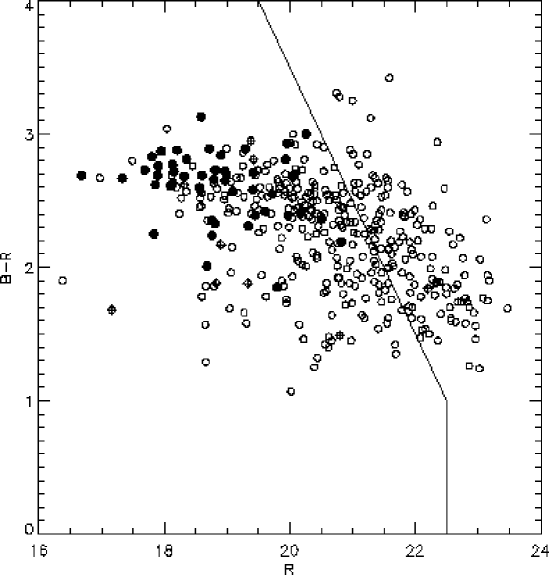
Fig. 4 shows the colour magnitude diagram for all the galaxies detected in the R-frame, and the corresponding magnitudes in the R and B bands were measured within the same apertures. The band of E/S0 sequence galaxies is discernable in Fig. 4; the spectroscopically confirmed cluster members are shown to fall mostly on the E/S0 sequence confirming that a large fraction of the galaxies on the E/S0 sequence belongs to the cluster. The mean error in B-R colour is $<0.08$.

Figure 4: A colour magnitude diagram for all galaxies detected in the R frame. The filled circles are for spectroscopically confirmed cluster members, and the crosses are for the non-members. The solid line gives the completeness limit.

2.3 Spectroscopy

Grism O300 was used for the spectroscopy. It has a zero deviation at 5900 Å, covers approximately 4700–7900 Å, and gives a dispersion of 3.59 Å$/$pixel ($0.314\arcsec$). The slit has a width of 2″, i.e. 6.4 pixels, yielding a resolution of $\sim$23 Å FWHM. Since there was only 1 frame per mask, cosmic rays were picked out individually by eye and replaced by the median of the surrounding pixels. The internal Helium and Argon lamps was used for wavelength calibration. The subsequent reduction was performed as described in Pierre et al. (1997). Redshifts were measured by a cross-correlation method implemented in the MIDAS environment following Tonry and Davis (1979). The cross-correlation results for each spectrum were checked independently by eye.

The results from the cross-correlation analysis for all spectra are presented in Table Probing the gravitational potential of a nearby lensing cluster Abell~2104. Heliocentric correction has not been applied, but is negligible at this resolution. The absolute error in the velocity calibration is $\sim 200$ km s^-1.

As a first guess, galaxies are considered to be cluster members if they lie within 3000 km s^-1 of the central cD galaxy, which selects 47 (the main sample) out of the 60 galaxies. This procedure eliminates most of the foreground and background galaxies without affecting the dispersion measurements significantly. If we relax the velocity constraint and apply the usual $3\sigma-$clipping technique then we have 51 cluster members (the extended sample). The cluster redshift distribution for both samples is displayed in Fig. 5. The histogram includes all galaxies in the redshift range $z\sim 0.135-0.175$ in Table Probing the gravitational potential of a nearby lensing cluster Abell~2104 and a Gaussian corresponding to the velocity distribution of the main sample. The bi-weighted mean and scale for the main sample are $z=0.1532^{+0.0004}_{-0.0006}$ and $\sigma=1148^{+190}_{-65}$ km s^-1 correspondingly; and $z=0.1538^{+0.0009}_{-0.0006}$ and $\sigma=1401^{+160}_{-130}$ km s^-1 for the extended sample. It is difficult to find an objective criterion for deciding which galaxies are cluster members. Even with the sophisticated weighting scheme employed by Carlberg et al. (1997), the determination of the weight for each galaxy is still subjective. In Table Probing the gravitational potential of a nearby lensing cluster Abell~2104, we have marked only the galaxies from the main sample as cluster members.

For the main sample we have enough redshifts to test whether or not the galaxy velocities are drawn from a Gaussian distribution applying various statistical tests for normality (e.g. D’Agostino & Stephens 1986; ROSTAT – Beers et al., 1990; Bird & Beers, 1993). As a result Anderson-Darling test (A²) accepts the hypothesis for normal distribution at 90% significance, the combined skewness and kurtosis test (B1 & B2 omnibus test) at 97% level and the alternative shape estimators, asymmetry index and tail index based on order statistics, were found to be $-0.21$ and $0.98$ respectively which also show that the velocity distribution is drawn from a Gaussian.

We can obtain a conservative estimate of the errors on the velocity dispersion by comparing the dispersion from the extended and main samples. When we take into account of the uncertainties in cluster membership, a more conservative estimate of the errors should give the velocity dispersion as $1200\pm 200$ km s^-1.

We also investigated the presence of substructures in ($\alpha$, $\delta$, $z$) space but no obvious signal was detected (see Fig. 6). More redshifts are required for a proper statistical analysis.

Figure 5: Cluster galaxy redshift histogram (bin size $\Delta z=0.0025$). The galaxies considered to be cluster members are marked as solid histogram while the dotted histogram are for the extended sample. The dashed curve is a Gaussian with parameters corresponding to the velocity distribution of the galaxies in the main sample.

Figure 6: Wedge diagrams showing the distribution of galaxies with measured redshifts.

3 X-ray Data

We have observed the cluster with the ROSAT HRI and the ASCA GIS and SIS detectors. The HRI has a high spatial resolution of $\sim 5\arcsec$, which provides a high resolution X-ray surface brightness profile, but it has no energy resolution. ASCA on the other hand has a low spatial resolution ($\sim 3\arcmin$) but relatively high energy resolution and high sensitivity in the energy range 1–10 keV, which provides a reliable gas temperature measurement for clusters of galaxies.

3.1 Spectral analysis

The cluster was observed with ASCA using both detectors of the Gas Scintillation Imaging Spectrometers (GIS) and Solid-state Imaging Spectrometers (SIS) in February 1996. The SIS detectors were operated in 1-CCD mode. The data was screened and cleaned according to the standard procedures recommended (The ABC guide to ASCA data reduction). The spectra were extracted from the central $\sim 6.5\arcmin$ radius from the GIS2 and GIS3 detectors, excluding one discrete source. Similarly, spectra were extracted from the central $\sim 3\arcmin$ radius from the SIS0 and SIS1 detectors. A standard blank-sky exposure screened and cleaned in the same way as the cluster field was used for background subtraction by extracting a background spectra from the same region on the detector as the cluster spectra. The spectra were grouped into energy bins such that the minimum number of counts before background subtraction was above 40, which ensures that $\chi^{2}$ statistics would still be valid. The 4 spectra from each detector were simultaneously fitted with a Raymond-Smith thermal spectra (Raymond & Smith 1977) with photoelectric absorption (Morrison & McCammon 1983) from the XSPEC package (Fig. 7). We adopted the abundance table with the relative abundance of the various elements from Feldman (1992). The free parameters were the gas temperature ($T_{g}$), Galactic neutral hydrogen absorption column density (N(H)), metal abundance (abund) and the emission integral. All 4 spectra were to have the same value for the free parameters except for the emission integral, since the GIS and SIS PSF were different and the extraction regions were smaller for the SIS spectra compared to that of the GIS. The two GIS spectra were assumed to have the same emission integral but different from the SIS emission integrals. Results of the best simultaneous fit to the 4 spectra along with fits to the individual spectra are tabulated in Table 1. Only data in the energy range where the effective area of the detectors are $>10$ cm² were used for the spectral fitting, i.e. 0.6–7.5 keV for SIS data and 0.85–10.0 keV for GIS data.

Figure 7: ASCA spectra from the 4 detectors GIS2, GIS3, SIS0, SIS1. The solid curves show the simultaneous fit to all 4 spectra using a Raymond-Smith model with photoelectric absorption. The model fits also take into account of the instrumental responses of the individual detectors.

Table 1: Results on spectral fit to ASCA data

	GIS	SIS	GIS+SIS	GIS*	SIS*	GIS+SIS*
kTg	$8.95^{+1.55}_{-1.24}$	$7.33^{+0.97}_{-0.71}$	$7.88^{+0.56}_{-0.52}$	$10.51^{+1.21}_{-1.12}$	$11.04^{+0.90}_{-1.21}$	$10.36^{+0.64}_{-0.65}$
abund	$0.21^{+0.11}_{0.12}$	$0.22^{+0.11}_{0.10}$	$0.32\pm 0.08$	$0.20\pm 0.13$	$0.23\pm 16$	$0.22\pm 0.07$
N(H)	$15.3\pm 4.7$	$22.5\pm 2.2$	$20.8\pm 1.6$	9.25	9.25	9.25
$\chi^{2}$	0.55	0.75	0.91	0.56	0.90	0.95

Notes:
kT_g - the gas temperature in keV;
abund - the fractional solar metal abundance;
N(H) - the neutral hydrogen column density in units of $10^{20}$ cm²;
$\chi^{2}$ - reduced $\chi^{2}$.
col. 2 - fit to the combined GIS data;
col. 3 - fit to the combined SIS data;
col. 4 - simultaneous fit to GIS2, GIS3, SIS0 & SIS1 spectra;
col. 5,6,7 - same as col. 2,3,4 respectively, but N(H) was fixed to the radio value and SIS data below 1 keV were not used.
The quoted errors for each parameter correspond to the 90% confidence range.

The neutral hydrogen column density derived from the ASCA data were 2 times larger than the N(H) ($=9.25\times 10^{20}$ cm²) measured from radio data by Starck (1992). If we try to fix N(H) to the value determined by Starck (1992), then there is obvious discrepancy between the model spectrum and the SIS data below 1 keV. Unfortunately, there is no PSPC data available for this cluster to place definitive constraints on the N(H) value. It is possible that there is a local over-density of absorbing neutral gas along the line-of-sight to the cluster, though it is more likely to be a calibration error for the SIS detector. Calibration of the low-energy part of the SIS detector is known to produce erroneous results such that it favours a high N(H) inconsistent with PSPC results (Schindler et al. 1998 & Liang et al. 2000). In view of the possible calibration error for the SIS, the data were also fitted with the above models with a fixed N(H) given by Starck (1992) by excluding the SIS data below 1 keV. The temperature thus deduced was significantly higher than before. In the following studies, we will adopt these parameters deduced from a simultaneous fit of data from the GIS detectors in the energy range 0.85 to 10 keV and the SIS detectors between 1 and 7.5 keV.

3.2 ROSAT HRI data

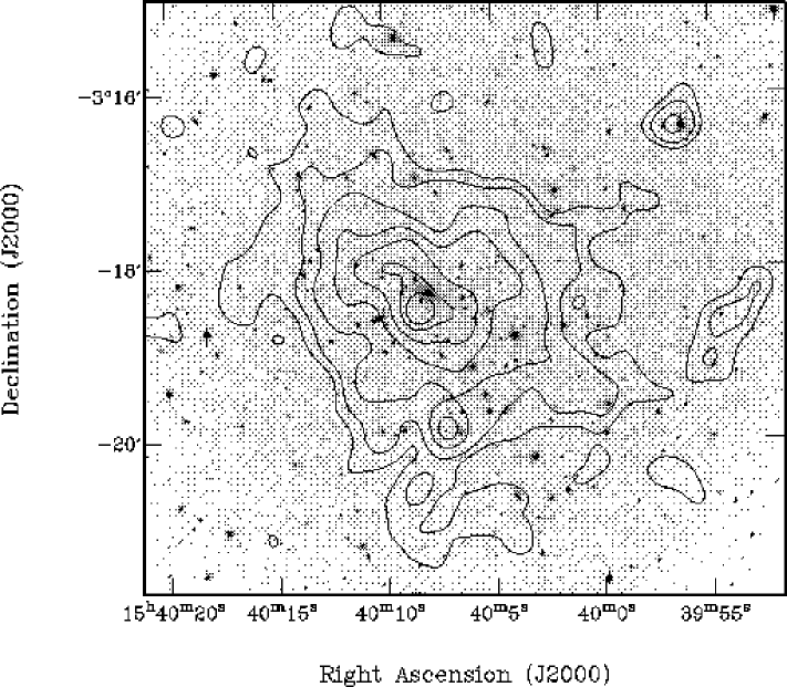
The cluster was observed by the ROSAT HRI in February (7.6ksec) and August (36ksec) 1996. The X-ray centroid was found to be 15:40:08.1 $-$03:18:17, which is $\sim 1\arcsec$ from the position of the cD galaxy 15:40:07.96 $-$03:18:16.7. The positional error for the X-ray centroid is $\sim 5\arcsec$, hence the small apparent displacement between the cD position and the X-ray centroid is insignificant. The X-ray surface brightness was obtained by extracting the photons in a radius of $7\arcmin$ and the background was extracted from an annulus of $8\arcmin-10\arcmin$ radius from the X-ray peak. Discrete X-ray sources were excluded from the extraction. There were 8 discrete X-ray sources in the HRI image. Fig. 1 shows the X-ray contours overlaid on the optical image of the cluster field. The X-ray image show significant substructure in the centre with an overall elliptical appearance. The discrete X-ray sources at 15:40:07.2 $-$03:19:53 is embedded in the cluster emission. The relative astrometry between X-ray and optical was checked using 4 of the discrete X-ray sources that had clear optical identification. The X-ray positions had a maximum displacement of $\sim 2\arcsec$ relative to the optical coordinates. The X-ray contours were adjusted to the optical coordinate system using the 4 discrete X-ray sources, which gave a relative astrometric accuracy of $\sim 0.5\arcsec$ between optical and X-ray coordinates.

A radial average of the X-ray surface brightness for the cluster is shown in Fig. 8. A best fit $\beta$ profile (Cavaliere and Fusco-Femiano 1976)

$$S_{x}(r)=S_{0}[1+(\frac{r}{r_{0}})^{2}]^{-3\beta+1/2}$$ (1)

convolved with the instrument PSF is shown as a solid curve superimposed on the data.

Figure 8: X-ray surface brightness from HRI data. The solid curve gives the best $\beta$ profile after convolution with the HRI PSF. The dashed horizontal line segment indicates the background level.

The best fit gave $\beta=0.50^{+0.02}_{-0.03}$ and $\theta=51^{+5}_{-6}\arcsec$. The uncertainties quoted are $1\sigma$. The total X-ray luminosity within the central $7\arcmin$ radius is $L_{x}\sim 8.95\times 10^{44}$ ergs s^-1 in the ROSAT band of 0.1–2.4 keV, assuming $N(H)=9.25\times 10^{20}$ cm², $kT_{g}=10.4$ keV (or $1.2\times 10^{8}$ K), and an abundance of 0.22. The X-ray luminosity thus deduced is consistent with that estimated from the ROSAT all-sky survey (Pierre et al. 1997). The corresponding bolometric X-ray luminosity is $L_{x}\sim 3\times 10^{45}$ ergs s^-1. The central electron density was thus derived to be $n_{e,0}\sim 5.92\times 10^{-3}$ cm^-3. The central cooling time for this cluster is $t_{cool}\sim 10^{10}$ yr, greater than a Hubble time.

4 Analysis

While the X-ray image show significant substructure in the cluster indicating deviations from hydrostatic equilibrium, the cluster total mass deduced from assumptions of dynamical equilibrium are still reliable, as is shown by numerical simulations (Evrard et al 1996 & Schindler 1996). Under the assumption of hydrostatic equilibrium and spherical symmetry, the cluster total mass is directly related to the intracluster gas properties as:

$$M_{tot}(r)=-\frac{rkT_{g}(r)}{\mu m_{p}G}(\frac{d\ln{n_{e}(r)}}{d\ln{r}}+\frac{d\ln{T_{g}(r)}}{d\ln{r}})$$ (2)

In general, a good fit can be found for the X-ray surface brightness distribution using the parametrisation given in Eqn. 1, which in turn gives the gas density as follows if the gas is isothermal:

$$\frac{n_{e}(r)}{n_{e,0}}=[1+(r/r_{0})^{2}]^{-3\beta/2}$$ (3)

Hence, the gravitational potential is given by

$$\phi(r)-\phi_{0}=\frac{3\sigma_{0}^{2}}{2}\ln{[1+(\frac{r}{r_{0}})^{2}]}$$ (4)

where $\sigma_{0}^{2}\equiv\beta kT_{g}/\mu m_{p}$ and the total mass is given by

$$M_{tot}(r)=(\frac{3\sigma_{0}^{2}r_{0}}{G})\frac{(r/r_{0})^{3}}{1+(r/r_{0})^{2}}$$ (5)

The lensing effects of the background galaxies by the cluster gravitational field is directly related to the 2-D projection of the total mass density. In this case, the projected total mass density is given by

$$\Sigma^{2D}_{tot}(r)=\frac{3\sigma_{0}^{2}}{4Gr_{0}}\frac{2+(r/r_{0})^{2}}{[1+(r/r_{0})^{2}]^{3/2}}.$$ (6)

If we consider galaxies as test particles in the cluster potential well, then Jean’s equation for a collisionless, steady state, non-rotating spherically symmetric system gives

$$M_{tot}(r)=-\frac{r\sigma_{r}^{2}(r)}{G}(\frac{d\ln{n_{gal}(r)}}{d\ln{r}}+\frac{d\ln{\sigma^{2}_{r}(r)}}{d\ln{r}}+2\beta_{t})$$ (7)

where $n_{gal}$ is the spatial galaxy number density, $\beta_{t}$ is the anisotropy index and $\sigma_{r}$ is the radial velocity dispersion. The spatial galaxy number density is related to the observed 2-D projection of the galaxy number density through the Abel inversion given by

$$n_{gal}(r)=-\frac{1}{2\pi}\int_{r}^{\infty}\frac{d\Sigma^{2D}_{gal}(R)}{dR}\frac{dR}{\sqrt{R^{2}-r^{2}}},$$ (8)

$\sigma_{r}$ and $\beta_{t}$ are related to the observed line-of-sight velocity dispersion $\sigma_{l}$ through

$$\Sigma^{2D}_{gal}(R)\sigma_{l}^{2}(R)=2\int_{R}^{\infty}n_{gal}(r)\sigma_{r}^{2}(r)[1-\frac{R^{2}}{r^{2}}\beta_{t}]\frac{rdr}{\sqrt{r^{2}-R^{2}}}$$ (9)

In the simple case, where the galaxy orbits are isotropic, Eqn. 7 is equivalent to Eqn. 2 with $\sigma_{r}^{2}$ replaced by $kT_{g}/\mu m_{p}$.

If we make a further simplification by assuming that not only the gas but also the galaxies are isothermal, i.e. $\sigma_{r}(r)$ is a constant, then we have

$$\frac{n_{e}(r)}{n_{e,0}}=(\frac{n_{gal}(r)}{n_{gal,0}})^{\beta_{s}}$$ (10)

where $\beta_{s}=\mu m_{p}\sigma_{r}^{2}/kT_{g}$. Given the above parametrisation for the X-ray surface brightness and the resultant expression for $n_{e}$ given by Eqn. 3, we deduce the spatial galaxy density distribution as

$$\frac{n_{gal}(r)}{n_{gal,0}}=[1+(r/r_{0})^{2}]^{-\alpha}$$ (11)

where $\alpha=3\beta/2\beta_{s}$. The observed line-of-sight velocity dispersion is trivially given by $\sigma_{obs}=\sigma_{r}$ and $\alpha=3\sigma^{2}_{0}/2\sigma^{2}_{obs}$.

Alternatively, if we simplify the case by assuming that the galaxy density distribution follows that of the total mass, i.e. mass-follows-light, then from Jean’s equation (Eqn. 7) we see that the galaxies can not be isothermal if the gas is isothermal and the X-ray surface brightness is parametrised as in Eqn 1. The radial velocity dispersion is given by

$$\sigma^{2}_{r}(r)=\frac{1+(r/r_{0})^{2}/2}{1+(r/r_{0})^{2}/3}\sigma^{2}_{0}$$ (12)

where again $\sigma^{2}_{0}\equiv\beta kT_{g}/\mu m_{p}$. The line-of-sight velocity dispersion $\sigma_{l}$ can be deduced from Eqn. 9. However, the measured velocity dispersion is an average of $\sigma_{l}$ within a certain radius:

$$\sigma_{obs}^{2}(<R)=\frac{3}{4}[\frac{1+2(R/r_{0})^{2}-\sqrt{1+(R/r_{0})^{2}}}{(R/r_{0})^{2}}]\sigma^{2}_{0}.$$ (13)

In the case of Abell~2104, we have the observables $S_{x}(R)$, $T_{g}$, $\Sigma_{gal}^{2D}(R)$, $\sigma_{obs}$. Since the ASCA PSF was too poor to deduce a meaningful temperature profile, we will assume that the gas is isothermal for the time being. In the following section we will study the cluster total mass deduced from the various methods and examine their consistency using the simple parametrised $\beta$-model given above.

4.1 Mass estimate from optical data

The projected galaxy density distribution is consistent with a wide range of models. The following family of parametrised functions

$$\Sigma_{gal}(r)=\Sigma_{gal,0}[1+(r/r_{0})^{2}]^{-k}$$ (14)

were fitted to the projected galaxy density distribution after background subtraction using the density of galaxies in the annulus $220\arcsec$ to $240\arcsec$ as background. If we fix the core radius to the X-ray determined value of $51\arcsec$, then we found the best fit to be $k=1$ ($\chi^{2}=9.3$ with 10 degrees of freedom), though $k=1/2$ to $3/2$ were also statistically consistent with the observed data. Note that $k=1/2,1,3/2$ corresponds to spatial galaxy distributions of the form given in Eqn. 11 with $\alpha=1,3/2,2$ respectively. The projected total mass density distribution given by Eqn. 6 was also statistically consistent with the projected galaxy density distribution ($\chi^{2}=9.66$ with 10 degrees of freedom), which means mass-follows-light is not excluded. The 2D projection of the functional form $(r/r0)^{-1}[1+(r/r0)]^{-2}$ (Navarro et al. 1996) was also found to be statistically consistent with the observed galaxy distribution. The projected galaxy distribution is shown in Fig. 9 along with the various model fits. The observed galaxy density distribution is still declining towards the edge of the image indicating a wider field is needed to reach the true “edge” of the cluster. The X-ray data show that the cluster extends at least out to a radius of $7\arcmin$ which is beyond the optical field of view for the current observation. A wider field of view would help to reject some of the above models.

Figure 9: The radially averaged galaxy number density distribution (with background). The curves show a number of statistically consistent model fits to the data points. The short-dashed, solid and long-dashed curves corresponds to the $k=1/2,1,3/2$ cases of the family of curves given by Eqn. 14. The dotted curve shows the 2D projection of the Navarro model (Navarro et al. 1996).

If we estimate the total mass distribution from the galaxy density distribution and velocity dispersion assuming that the galaxies are isothermal, then $\sigma^{2}_{0}=(2\alpha/3)\sigma^{2}_{obs}$ where the observed data give $\alpha\sim 1$ to $\sim 2$ and $\sigma_{obs}=1200\pm 200$ km s^-1, implying that $\sigma_{0}\sim 823$ to $\sim 1625$ km s^-1. Thus from Eqn. 5 the total mass is between $3.5\times 10^{14}M_{\sun}$ and $13.4\times 10^{14}M_{\sun}$ within a radius of $220\arcsec$ (or 0.76 Mpc), and between $6.8\times 10^{14}M_{\sun}$ and $2.6\times 10^{15}M_{\sun}$ extrapolating to $7\arcmin$ (or 1.46 Mpc). Note that optical data alone does not constrain the mass very well, even under assumptions such as isothermality of the galaxy distribution and isotropy of the orbits.

On the other hand, if the galaxy distribution is not isothermal but follows that of the mass then the measured velocity dispersion implies that $\sigma_{0}\sim 1010\pm 165$ km s^-1 from Eqn. 13 and the total mass is $\sim(10.2\pm 3.7)\times 10^{14}M_{\sun}$ within a radius of $7\arcmin$ (or 1.46 Mpc).

4.2 Mass estimate from X-ray data

The values of $\beta\sim 0.5^{+0.02}_{-0.03}$, $r_{0}\sim 51^{+5}_{-6}\arcsec$ and $T_{g}\sim 10.4\pm 0.6$ keV have been determined from spatial analysis of the HRI data and the spectro-analysis of the ASCA data respectively. Thus from the X-ray data, $\sigma_{0}^{2}\equiv\beta kT_{g}/\mu m_{p}$ implies a $\sigma_{0}\sim 895\pm 45$ km s^-1 and a X-ray deduced total mass of $\sim(8.0\pm 0.8)\times 10^{14}M_{\sun}$ out to a radius of $7\arcmin$ (or 1.46 Mpc).

Note that if the galaxies are isothermal, then the X-ray deduced mass is consistent with the optically deduced mass (or generalised “Virial” mass) if $\alpha\sim 1$. The X-ray and optical data are also marginally consistent if mass-follows-light.

The total gas mass within $7\arcmin$ was found to be $\sim 7.8\times 10^{13}M_{\sun}$ which gives a gas fraction of $\sim 10$% compared to the X-ray deduced mass, but 5–10% compared to the dynamically deduced mass. The gas fraction within a radius of $r_{500}=1.14$ Mpc (where the over-density is 500 times the critical density of the Universe) is $\sim 8$%, which is lower than the average gas fraction of $(20\pm 1.9)$% for nearby hot ($kT_{g}>4$ keV) non-cooling flow clusters (Arnaud & Evrard 1999). The gas fraction within a radius of 1.46 Mpc gives a lower limit to the baryonic fraction. Since the baryonic matter density predicted from the Big Bang nucleosynthesis gives $\Omega_{b}\sim 0.04-0.06$ (Walker et al. 1991) from the measured light element abundance, the lower limit of the baryonic fraction of this cluster is thus consistent with $\Omega_{M}\leq 1$.

5 Discussions

For the above simple models, we have shown that the X-ray deduced mass is consistent with that from the optical data over the scale of 1–3 Mpc under the assumptions of dynamic equilibrium. In a recent paper by Lewis et al. (1999), they also found the X-ray and dynamically deduced mass were consistent for a sample of CNOC clusters at $z\sim 0.3$.

On the other hand, in a study of a sample of clusters with giant arcs, Allen (1998) found that the X-ray deduced mass was consistent with the position of the giant arcs for cooling flow clusters but $2-3$ times smaller than the lensing mass for non-cooling flow clusters. This was then explained as a direct consequence of the theory that cooling flow clusters were dynamically more relaxed than non-cooling flow clusters since cluster mergers would certainly disrupt a cooling flow. The cooling time for Abell~2104 is $t_{cooling}\sim 10^{10}$ yr at the centre, thus there is no evidence for a cooling flow in this cluster. Pierre et al. (1994) found a red tangential arc $7\aas@@fstack{\prime\prime}2$ from the centre of the cD galaxy (see Fig. 2). They found that the projected mass within the arc to be $6\times 10^{12}M_{\sun}$. Here we examine if the arc feature is consistent with the simple cluster potential deduced from the X-ray data. Since the projected density must reach the critical value at $7\aas@@fstack{\prime\prime}2$, it requires $\sigma_{0}\sim 1380-1175$ km s^-1 for an arc redshift in the range $z_{arc}\sim 0.5-3$ assuming the potential is spherically symmetric. However, the X-ray data gave $\sigma_{0}\sim 895\pm 45$ km s^-1 apparently inconsistent with the lensing deduced value, indicating that in this very simplistic model the X-ray mass within the arc radius appears to be $\sim 1.5-2$ times smaller than needed to produce the giant arc. Our result appears to be consistent with the results of Allen (1998). However, since the model we have adopted so far is very simple and the arc radius is relatively small ($7\aas@@fstack{\prime\prime}2$), it is premature at this stage to suggest that the lensing results are inconsistent with the X-ray data under the assumptions of hydrostatic equilibrium and isothermal gas. As it was pointed out in Pierre et al. (1994), the small arc radius is an indication that the local cD potential is probably as important as the global cluster potential in forming the arc feature. Indeed for most clusters with giant arcs, the arc radii are barely larger than the PSPC resolution and probably a few times larger than the HRI resolution, hence an inconsistency between X-ray deduced mass from simple models and that of the strong lensing deduced mass are not sufficient to prove that the cluster is not in dynamic equilibrium. An alternative explanation for the results of Allen (1998) could be that the cooling flow clusters are well modelled by a cluster potential similar to the type given by Eqn. 4, but non-cooling flow clusters have a different shape of gravitational potential, e.g. a mass profile that has a broad component in the outer parts of the cluster (e.g. Gioia et al. 1998). It would be difficult for the HRI to reject a model of this kind since it has a high background level and it would be easy to “hide” faint diffuse emission at large radii. In our study of Abell 2104, the current optical image does not extend to the extent of the X-ray emission, thus we need wide-field imaging to find out the true extent of the cluster.

The X-ray emission in the centre of the cluster shows strong ellipticity, the effect such asphericity has on the mass estimates needs to be addressed since the mass estimates given above were calculated under the assumption of spherical symmetry. Neumann & Böhringer (1997), estimated the effects of asphericity on mass estimates of CL0016+16, and found that the total mass was only changed by $\sim 2\%$ when the ellipticity was taken into account. The ellipticity demonstrated in the X-ray image of Abell~2104 is no stronger than that of CL0016+16.

So far we have only considered the isothermal gas models, but the total mass given by Eqn. 2 is more sensitive to $T_{g}$ than $n_{e}$. It is necessary to explore models with a temperature gradient. Markevitch et al. (1998) found an almost universal decrease in temperature in the outer regions over a radius of 0.3 to 1.8 Mpc in a sample of 30 nearby clusters ($0.04<z<0.09$). They found that for a typical 7 keV cluster, the observed temperature profile can be approximated by a polytropic equation of state with $\gamma\sim 1.2-1.3$. If we assume that Abell~2104 has a similar large scale temperature profile, then we can quantify the mass ratio between the polytropic and isothermal models as

$$\frac{M^{poly}_{tot}(r)}{M^{iso}_{tot}(r)}=\gamma(\frac{n_{e}(r)}{n_{e,0}})^{\gamma-1}.$$ (15)

Since the X-ray emissivity has only a weak dependence on $T_{g}$ over the 1–10 keV range (only a 10% change), the X-ray surface brightness varies insignificantly with $T_{g}$. We can then safely take the gas distribution as determined from the isothermal case (i.e. Eqn. 3). Thus at $7\arcmin$ radius (1.46 Mpc), a model with such a temperature gradient would give a mass that is $\sim 0.6$ times smaller than the isothermal case. This would cause the X-ray deduced mass to be strongly inconsistent with the dynamically deduced mass unless $\sigma_{r}^{2}$ increases with radius in a similar manner as $T_{g}$. Note that a temperature profile that decreases with the radius would also increase the total mass in the inner cluster regions compared to the isothermal model, and thus alleviate the discrepancy between the X-ray mass within the arc radius and the position of the giant arc. Fig. 10 shows the range of mass profiles deduced from the various methods and models discussed in the paper.

Figure 10: A comparison of 3D total mass distribution derived by the various methods. The solid curves give the range of X-ray deduced mass for isothermal gas; the dotted curves give the range of mass for the polytropic model. The dashed curves give the range of dynamic mass derived from the galaxy density distribution and velocity dispersion. The curves are plotted only for regions were data is available. The two stars show the range of mass estimates deduced from the position of the lensing arc.

6 Conclusions and Future prospects

The rich cluster Abell~2104 at a redshift of $z=0.1533$ was found to have a high X-ray luminosity ($\sim 9.0\times 10^{44}$ ergs s^-1 in [0.1-2.4] keV) and temperature ($10.4\pm 0.6$ keV) from ROSAT HRI and ASCA data. The central cooling time, $t_{cool}\sim 10^{10}$ yr for this cluster indicates the absence of a cooling flow. The galaxy velocity distribution showed that the cD galaxy was at rest at the bottom of the cluster potential. The X-ray image shows significant substructure in the centre of the cluster and an overall elliptical appearance. It appears that the cluster has not yet reached dynamical equilibrium.

As shown in Evrard et al (1996) and Schindler et al. (1996), the total mass deduced from assumptions of dynamical equilibrium are not significantly different from the true values. The total mass deduced from the X-ray data assuming hydrostatic equilibrium is consistent with the dynamic mass deduced from Jean’s equation. However, the current data on the projected galaxy density distribution and our knowledge of the galaxy orbits are limited for studies of cluster dynamics, which allows a wide range of possible parametric functions for the spatial galaxy density distribution without even attempting the non-parametric methods of Merritt and Tremblay (1994) or considering any anisotropic orbits. This can be improved by a deep wide-field observation, to extend the galaxy number density distribution to a large radius (up to 3 Mpc) and to allow a direct measure of the cluster mass from a weak shear analysis. This would allow us to definitively address the issue of whether or not the cluster is in dynamical equilibrium and constrain the range of possible total mass distributions allowed by the wide-range of data from lensing effects to X-rays. In order not to bias the results and incorporate a wide-range of the possible total mass density distributions, a non-parametric method should also be employed. With the launch of XMM and Chandra, we will soon able to obtain a temperature profile and probe the X-ray emission at the edge of the cluster which is crucial to the improvement of the X-ray mass estimates.

Table 2: Spectral analysis of Abell~2104

ID	RA(J2000)	Dec(J2000)	$z$	$\Delta V$	Q	R	$\Delta$R	B	$\Delta$B	member
102	15:39:53.0	-03:18:45.0	0.1504(*)	216	1	19.80	0.02	21.65	0.03	Y
103	15:39:53.8	-03:19:13.4	0.0068	178	2	20.80	0.03	22.29	0.03	N
105	15:39:56.1	-03:18:36.7	0.1552	179	2	20.08	0.02	22.78	0.06	Y
106	15:39:57.5	-03:19:41.9	0.1663	195	1	19.09	0.01	21.66	0.03	Y
107	15:39:58.9	-03:17:20.0	0.1456	154	1	18.59	0.01	21.72	0.04	Y
108	15:39:59.7	-03:19:35.8	0.1664	137	2	18.13	0.01	20.76	0.03	Y
109	15:40:00.6	-03:18:34.2	0.1561	254	2	18.68	0.01	20.69	0.02	Y
110	15:40:02.2	-03:17:23.3	0.1496	126	2	17.90	0.01	20.66	0.02	Y
111	15:40:03.1	-03:20:11.0	0.1585	174	2	17.83	0.01	20.08	0.01	Y
112	15:40:04.0	-03:18:46.8	0.1557	123	2	17.33	0.01	20.00	0.02	Y
113	15:40:05.4	-03:19:27.1	0.1526	152	2	18.35	0.01	21.16	0.03	Y
114	15:40:06.4	-03:18:19.8	0.1498	211	2	19.42	0.01	22.13	0.05	Y
115	15:40:07.9	-03:18:15.8	0.1536	154	1	16.68	0.00	19.37	0.01	Y
116	15:40:08.5	-03:18:06.1	0.1499	126	2	18.57	0.01	21.15	0.03	Y
117	15:40:10.2	-03:18:33.5	0.0367(*)	296	2	17.16	0.00	18.84	0.01	N
118	15:40:11.2	-03:17:56.4	0.1544	108	1	18.99	0.01	21.69	0.03	Y
119	15:40:12.4	-03:18:48.6	0.1555	142	2	18.96	0.01	21.68	0.03	Y
120	15:40:13.7	-03:18:02.2	0.1545	120	2	18.13	0.01	20.90	0.03	Y
123	15:40:18.7	-03:17:28.0	0.1656	249	2	18.76	0.01	21.11	0.02	Y
124	15:40:19.4	-03:18:08.3	0.1648	143	2	18.31	0.01	20.99	0.03	Y
125	15:40:20.7	-03:17:48.1	0.1586	196	1	18.90	0.01	21.74	0.04	Y
127	15:40:23.3	-03:18:52.9	0.2413	249	2	19.42	0.01	22.23	0.05	N
202	15:39:49.8	-03:16:45.5	0.1467	232	1	18.72	0.01	21.61	0.04	Y
204	15:39:52.3	-03:16:18.5	0.1526	130	1	17.80	0.01	20.63	0.02	Y
207	15:39:56.1	-03:18:30.2	0.1502	259	2	20.08	0.02	22.78	0.06	Y
211	15:40:01.2	-03:20:24.7	0.1557	143	1	20.20	0.02	22.22	0.04	Y
213	15:40:03.3	-03:18:35.3	0.1505	102	2	20.19	0.02	22.61	0.05	Y
214	15:40:04.4	-03:19:37.2	0.1476(*)	219	2	18.97	0.01	21.62	0.03	Y
215	15:40:05.2	-03:19:39.0	0.1523	126	1	18.32	0.01	21.00	0.03	Y
216	15:40:05.9	-03:19:07.7	0.1531	124	2	17.89	0.01	20.58	0.02	Y
217	15:40:07.3	-03:18:59.8	0.1577	115	1	18.76	0.01	21.00	0.02	Y
218	15:40:08.3	-03:18:20.5	0.1059	199	2	18.32	0.01	20.94	0.03	N
219	15:40:09.9	-03:18:56.5	0.1624	159	1	18.56	0.01	21.16	0.02	Y
220	15:40:10.4	-03:16:39.0	0.1580	110	1	17.95	0.01	20.82	0.02	Y
221	15:40:11.6	-03:16:54.5	0.1489	106	2	19.41	0.01	21.99	0.04	Y
223	15:40:16.6	-03:18:09.4	0.1493	99	2	19.72	0.02	22.27	0.05	Y
224	15:40:19.1	-03:19:41.9	0.1490	198	1	18.79	0.01	21.45	0.03	Y
225	15:40:20.3	-03:18:52.2	0.1601	183	1	18.81	0.01	21.14	0.03	Y
227	15:40:21.8	-03:16:25.3	0.1449	171	2	20.05	0.02	22.73	0.06	Y
228	15:40:23.5	-03:18:00.4	0.1436	239	2	20.26	0.02	23.26	0.10	Y
302	15:39:50.5	-03:20:49.9	0.1522	204	1	19.45	0.01	21.84	0.04	Y
304	15:39:52.4	-03:19:33.2	0.0122	228	2	22.20	0.06	24.04	0.10	N
306	15:39:54.8	-03:19:09.5	0.1545	132	1	18.60	0.01	21.29	0.03	Y
311	15:40:00.4	-03:20:32.3	0.1516	196	2	19.61	0.02	22.03	0.04	Y
312	15:40:01.7	-03:18:40.0	0.1498	122	2	18.15	0.01	20.87	0.02	Y
313	15:40:02.5	-03:16:36.5	0.1084(*)	195	2	18.90	0.01	21.07	0.02	N
314	15:40:04.0	-03:20:38.4	0.1552	115	2	17.86	0.01	20.48	0.02	Y

ID	RA(J2000)	Dec(J2000)	$z$	$\Delta V$	Q	R	$\Delta$R	B	$\Delta$B	member
315	15:40:05.1	-03:18:29.5	0.1529	228	1	18.81	0.01	21.54	0.03	Y
316	15:40:06.2	-03:18:27.4	0.1577	216	2	19.95	0.02	22.88	0.07	Y
317	15:40:07.6	-03:17:06.7	0.1530	161	1	19.29	0.01	22.18	0.05	Y
318	15:40:08.5	-03:16:56.3	0.1577	132	1	18.20	0.01	21.08	0.03	Y
319	15:40:10.1	-03:19:52.0	0.1573	152	1	19.34	0.01	21.65	0.03	Y
320	15:40:11.4	-03:20:46.7	0.2004(*)	153	2	18.83	0.01	20.71	0.01	N
321	15:40:12.0	-03:20:21.1	0.0706	213	2	19.33	0.02	21.21	0.03	N
323	15:40:15.0	-03:16:48.0	0.1535	190	2	19.93	0.02	22.74	0.06	Y
324	15:40:16.6	-03:19:45.8	0.1635	154	1	19.97	0.02	22.36	0.05	Y
325	15:40:17.2	-03:21:00.7	0.1531	177	2	17.69	0.01	20.42	0.02	Y
327	15:40:19.4	-03:20:42.4	0.1503	173	1	18.10	0.01	20.71	0.03	Y
328	15:40:20.8	-03:18:15.1	0.2849	181	2	19.38	0.01	22.33	0.06	N
329	15:40:22.6	-03:18:14.8	0.1557	251	1	20.82	0.03	23.01	0.07	Y

Notes:
Column 1: internal reference number to Fig. 3.
Column 2 & 3: RA and Dec (J2000). Galaxy positions were determined from the R image and should have an accuracy of $\sim$ 0$\aas@@fstack{\prime\prime}$7 rms.
Column 4: redshift
(*) signifies the presence of emission lines:
     102: H$\beta$, H$\alpha$, [N ii], [S ii]
     117: H$\beta$, [O iii], H$\alpha$, [N ii], [S ii]
     214: H$\beta$, H$\alpha$
     313: H$\beta$, H$\alpha$, [N ii], [S ii]
     320: He i, H$\alpha$, [N ii], [S ii]
     214: [O ii], [O iii], H$\beta$ , H$\alpha$, [N ii], [S ii]
Column 5: $\Delta V$ is the internal measurement error and is related to the correlation coefficient $C_{corr}$ by the formula $\Delta V=k/(1+C_{corr})$ where $k\sim 870$ km s^-1 was determined by the Tonry and Davis (1979) method.
Column 6: redshift measurement quality:
     1: highest peak in the correlation function and checked by hand,
     2: highest peak in the correlation function but unable to be checked by hand.
Column 7, 8, 9 & 10: R, $\Delta$R, B and $\Delta$B magnitudes:
Column 11: Cluster member galaxy (within $\pm 3000$ km/s of the cD galaxy).