Fast CMB Analyses via Correlation Functions

Abstract

We propose and implement a fast, universally applicable method for extracting the angular power spectrum ${\cal C}_{\ell}$ from CMB temperature maps by first estimating the correlation function $\xi(\theta)$. Our procedure recovers the ${\cal C}_{\ell}$’s using $N^{2}$ (but potentially $N\log N$), operations, where $N$ is the number of pixels. This is in contrast with standard maximum likelihood techniques which require $N^{3}$ operations. Our method makes no special assumptions about the map, unlike present fast techniques which rely on symmetries of the underlying noise matrix, sky coverage, scanning strategy, and geometry. This enables for the first time the analysis of megapixel maps without symmetries. The key element of our technique is the accurate multipole decomposition of $\xi(\theta)$. The ${\cal C}_{\ell}$ error bars and cross-correlations are found by a Monte-Carlo approach. We applied our technique to a large number of simulated maps with Boomerang sky coverage in $81000$ pixels. We used a diagonal noise matrix, with approximately the same amplitude as Boomerang. These studies demonstrate that our technique provides an unbiased estimator of the ${\cal C}_{\ell}$’s. Even though our method is approximate, the error bars obtained are nearly optimal, and converged only after few tens of Monte-Carlo realizations. Our method is directly applicable for the non-diagonal noise matrix. This, and other generalizations, such as minimum variance weighting schemes, polarization, and higher order statistics are also discussed.

1. Introduction

Future missions of measuring the Cosmic Microwave Background (CMB) fluctuations will revolutionize our knowledge of cosmology. They will either confirm or refute the basic Big Bang paradigm, will reveal the values of most cosmological parameters within a few percent (e.g., Spergel 1994, Knox 1995, Hinshaw, Bennett, & Kogut 1995, Jungman et al. 1996, Zaldarriaga, Spergel, & Seljak 1997, Bond, Efstathiou, & Tegmark 1997). The large number of pixels contained in current and future experiments enable these exciting developments, but at the same time, present unprecedented challenges the data analysis. The mainstream maximum likelihood techniques are already pushed to their limits by the largest existing CMB maps, but they are clearly inadequate for future megapixel surveys. Therefore the most important near term task for CMB research is to find techniques which could perform the required analyses with realistic resources, thus fulfill the promise of the high precision experiments.

This Letter proposes a fast, universally applicable method for the estimation of $C_{l}$’s from any CMB pixel map, based on estimating correlation functions. The recovered errorbars are at most $10\%$ larger than the theoretically smallest possible ones imposed by cosmic variance and noise. Optimal methods could further decrease these errorbars only slightly, and at an unrealistic cost; thus they represent a case of diminishing returns. Our procedure scales as $N^{2}$, and more sophisticated algorithms will improve this to $N\log N$. This essentially solves the problem for two major upcoming space missions, MAP (Microwave Anisotropy Probe) and the Planck, and at the same time allows more detailed analyses of current and future balloon-borne and ground based experiments. The short analysis turn around time enables Monte-Carlo (MC) studies of systematics, foregrounds, errors, underlying models etc. These are essential to the interpretation of the data but inaccessible to present methods.

The standard maximum likelihood methods for analyses were developed and tested on COBE measurements (e.g., Górski 1994, Górski et al. 1994, 1996, Bond 1995, Tegmark & Bunn 1995, Hinshaw et al. 1996, Tegmark 1996, Bunn & White 1996, Bond, Jaffe, & Knox 1998, hereafter BJK98, 2000) which have only about $N\simeq 1000$ pixels. Balloon-borne experiments, such as Boomerang (de Bernardis et al. 2000), Maxima (Hanany et al. 2000), and Tophat (Martin et al. 1996), and ground based measurements e.g., TOCO (Miller et al. 1999) and Viper (Peterson et al. 2000) with up to $N\simeq 10^{5}$ are already pushing present day supercomputer technology. The future missions MAP and Planck with $N=10^{6}-10^{7}$ are estimated to require up to millions of years (Borrill 1999, Bond, Crittenden, Jaffe, & Knox 2000) for one iteration of the quadratic maximum likelihood estimator for $C_{l}$’s. The disk storage and memory usage of these algorithms are prohibitive as well.

To date fast algorithms were presented under two fairly restrictive assumptions: i) the noise is both temporally uncorrelated and spatially axially symmetric ii) the foregrounds can be exactly removed both from the map and the correlation matrix (Oh, Spergel, & Hinshaw 1999, Wandelt, Hivon & Gorski 1998, 2000). Our approach is significantly different from these, since it does not assume any symmetries.

2. Description of the Method

,

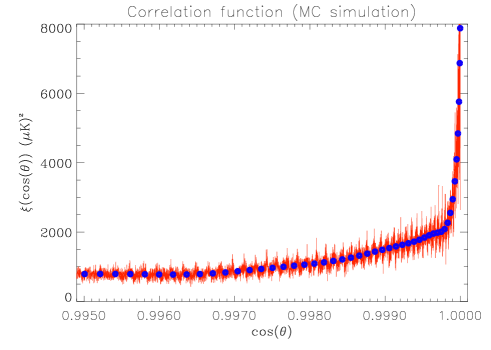
Figure 1.— The left panel displays a typical high resolution measurement of the two-point correlation function along with its Gaussian resampling at Legendre roots (large dots). The singular feature at around $1$ degree ($\cos\theta\simeq 0.9998$) condenses most of the information about the $C_{l}$’s. The right panel present a few examples of the inversion process. Individual $C_{l}$’s are calculated from the correlation function with the method described in the paper.

The basic steps of our recipe to extract $C_{l}$’s from a large CMB map are conceptually simple: first we measure the two-point correlation function in high resolution bins, next we smooth it with Gaussian kernels centered on the roots of Legendre polynomials, finally, we integrate to obtain the $C_{l}$’s. Each step is fine-tuned in order to arrive at a fast method, which is as precise as possible.

Let us denote the temperature fluctuations at a sky vector $q$, a unit vector pointing to a pixel on the sky, with $T(q)$. In isotropic universes the two-point correlation function is a function only of the angle between the two vectors and can expanded into a Legendre series,

$$\xi_{12}=\langle{T(q_{1})T(q_{2})}\rangle=\sum_{\ell}\frac{\ell+1/2}{\ell(\ell+1)}{\cal C}_{\ell}P_{\ell}(\cos\theta),$$ (1)

where $\cos\theta=q_{1}.q_{2}$, the dot product of the two unit vectors, $P_{\ell}(x)$ is the $\ell$-th Legendre polynomial, and the ${\cal C}_{\ell}$ coefficients realize the angular power spectrum of fluctuations. If the CMB anisotropy is Gaussian, which is expected to be an excellent approximation, the correlation function, or the ${\cal C}_{\ell}$’s yield full statistical description.

In reality each pixel value, $\Delta_{i}$, contains contributions from the CMB and noise; the latter is also assumed to be Gaussian with a correlation matrix (the noise matrix) $N_{ij}$, determined during map-making. The full pixel-pixel correlation matrix is $C_{ij}=\xi_{ij}+N_{ij}.$ We adopted the edge and noise corrected estimator of Szapudi & Szalay (1998),

$$\tilde{\xi}(\cos\theta)=\sum_{ij}f_{ij}(\Delta_{i}\Delta_{j}-N_{ij}),$$ (2)

where $f_{ij}=0$ unless the pair of pixels belong to a particular bin in $\cos\theta$, and $\sum_{ij}f_{ij}=1$. The above estimator is unbiased, i.e. $\langle{\tilde{\xi}(\cos\theta)}\rangle=\xi(\cos\theta)$. A complex pair weighting might be required in surveys with uneven coverage, and to optimize the performance of the estimator (see discussions in §4). For this Letter we used a straightforward $N^{2}$ program to estimate the above quantity in a large number of bins linear in $\theta$ massively oversampling the pixel separation. The results are robust against the exact number of bins used, for the measurements presented here we have placed $300,000$ bins in the range of $0-\pi$.

The raw correlation function is then resampled with a Gaussian filter with additional weighting proportional to the number of pairs in each bin. The centers of the filters are determined by the roots of the Legendre polynomial $P_{\ell_{max}}$ of the highest $\ell_{max}$ to be measured; their widths is about half the pixel size. This procedure allows accurate centering of the filters, suppresses any high frequency sub-beam measurement noise due to the massive oversampling. The Gaussian convolution translates into a simple multiplication in $\ell$-space, thus easy to correct for. We verified that, after this correction, the final result is robust against varying the size of the filter; we have used $4^{\prime}$. For small surveys, a smooth cut-off of the correlation function is necessary on large angles to suppress noise from edge effects. We checked that the ${\cal C}_{\ell}$’s are robust against changing the scale and sharpness of the cut-off (up to a corresponding smoothing in $\ell$-space); we have used exponential tapering above $18^{\circ}$. The left panel of Figure 1 shows an example of a measured correlation functions along with its resampled version (large dots). The ${\cal C}_{\ell}$’s are determined from the resampled correlation function by Legendre-Gauss integration (e.g., Press et al. 1992). Since this is exact up to $2\ell_{max}+1$, the ${\cal C}_{\ell}$’s are as accurately recovered as the correlation function. The right panel of Figure 1 shows examples of ${\cal C}_{\ell}$’s inverted from two-point correlation function measurements in simulations.

The full correlation matrix of the above estimator can be calculated analytically as well. Under Gaussian assumption, the cross-correlation between two bins denoted with $1$ and $2$, respectively is $\langle{\delta\xi_{1}\delta\xi_{2}}\rangle=\sum_{ijkl}f^{1}_{ij}f^{2}_{kl}[\xi_{ik}(\xi_{jl}+N_{jl})+k\leftrightarrow l)].$ The straightforward calculation of the above expression takes $N^{4}$ operations, thus infeasible for a megapixel survey. While this scaling is likely to be improved to $N(\log N)^{3}$ with the advanced algorithms in the near future, in this Letter we propose an entirely different approach: high volume MC simulations. Certain systematics can only be taken into account this way, and the speed of our method makes such computations possible.

3. Simulations

,

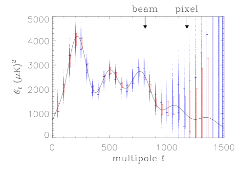
Figure 2.— The left panel displays the main results of this Letter: ${\cal C}_{\ell}$’s calculated in 1298 Boomerang-like simulations and then rebinned into flat ${\cal C}_{\ell}$-bands with width of $50$. The small points show the individual measurements with errorbars representing the standard deviations in each band. Theoretical errorbars of Equation 3 are displayed shifted to the right for clarity. The comparison shows that our method is unbiased, and has nearly optimal variance. The arrows point to the effective beam and pixel scales. The right panel shows the distribution of measurements in selected bands. Shifted lognormal (dash) and Gaussian curves are fitted to the histogram. Except for the $\ell=50$ band, the two are indistinguishable. Horizontal lines display optimal FWHM dispersion for comparison.

To illustrate the method, we generated $1298$ MC realizations of CMB maps with a standard CDM power spectrum and typical instrumental noise. The sky coverage used to create the maps ($\sim 1000\,{\rm deg}^{2}$), the noise level ($\sim 45\,\mu{\rm K}$ per pixel), and the Gaussian beam size ($10^{\prime}$ FWHM) were comparable to the BOOMERanG experiment (de Bernardis et al. 2000). Full sky maps in $\sim 7^{\prime}$ pixels were generated by the HEALPix (Gorski et al. 1998) synfast routine. Then maps were reduced to the desired coverage, and uniform white noise has been added.

The angular power spectra have then been extracted, corrected for beam, pixelization, and the additional $4^{\prime}$ smoothing of the correlation function, and finally averaged into flat band-powers ${\cal C}_{\bar{\ell}}$ with widths $\Delta\ell=50$ and positions $\bar{\ell}$ that of de Bernardis et al. (2000). Figure 2 shows ${\cal C}_{\bar{\ell}}$ for all realizations, together with the corresponding error bars. They are to be compared with the optimal error bars computed from the approximate formula

$$\Delta{\cal C}_{\ell}=\sqrt{\frac{2}{(2\ell+1)f_{sky}}}\left({\cal C}_{\ell}+w^{-1}\ell(\ell+1)W^{-2}_{\ell}/2\pi\right),$$ (3)

where $f_{sky}$ is fraction of the sky observed, $w^{-1}$ is the noise variance and $W_{\ell}$ is the beam of the experiment. According to Figure 2, our estimator is nearly optimal and unbiased. In any given $\bar{\ell}$-band, the differences between the measured and theoretical mean and variance are at most $10\%$ of the optimal variance. The MC method for determining the errorbars converges remarkably fast: a few tens of realizations give an accurate estimate of both the mean and variance. For real data, the smoothed measured ${\cal C}_{\ell}$’s themselves should be taken for generating MC realizations.

In addition, we have estimated the cross-correlations between bands, and found them to be consistent with zero, decreasing as $\simeq 3/\sqrt{N_{r}}$ with the number of realizations $N_{r}$. These experiments show that our method does not induce spurious correlations into the measurements.

The right panel of Figure 2 displays distributions of several recovered band-powers, illustrating different regimes of signal or noise domination of the total variance. We found that the distribution in all bands is well fitted with an offset lognormal probability density (BJK98), although it is indistinguishable from a Gaussian in most bands.

In summary, our method has nearly identical mean, variance, cross-correlations, and distribution as one would expect from standard maximum likelihood methods. The present implementation of the above pipeline takes about 25 minutes of serial CPU on a small workstation, including artificial map generation, measurement of the correlation function, and estimating the $C_{l}$’s individually, and finally summarizing them into band-powers. The required time is dominated by the measurement of the two-point correlation function (about 20 minutes); obtaining the $C_{l}$’s from it is negligible (few seconds).

These measurements illustrate that pairwise estimators with heuristic weights are feasible, their speed is far superior to maximum likelihood techniques, and they can be rendered nearly optimal. While details of the above recipe are subject to honing for future practical applications, our present code is capable of analyzing MAP on a sub-supercomputer class CPU without explicit reliance on symmetries; a feat no other method could claim.

4. Discussion

We presented a novel method to extract ${\cal C}_{\ell}$’s from large CMB maps via two-point correlation functions. We have cast our determination of ${\cal C}_{\ell}$ into 3 steps: fine-grained $C(\theta)$ estimation, the pixel-related $4^{\prime}$ Gaussian smoothing of it, followed by $P_{\ell}$ multiplication and Gauss-Legendre integration. The resulting expression for ${\cal C}_{\ell}$ can be itself understood as a sum over pixel pairs, with a pair-weighting proportional to the Gaussian smoothing of $P_{\ell}$. In this respect our estimator belongs to the class of quadratic estimators for ${\cal C}_{\ell}$, of which other examples (e.g., BJK98) have been used in the past and are expected to give similar results.

In the present example the measured errorbars were at most $10$% larger then the theoretically minimal ones; this negligible suboptimality allowed the reduction of the CPU time from months (Borrill 1999, Table 3) to hours. For future large missions the difference will be even more dramatic: optimal methods would improve the errorbars only slightly at a prohibitive cost.

Our new approach has several advantages in comparison to previous techniques. It scales as $N^{2}$ even in its most straightforward implementation, compared to typical quadratic estimators which scale as $N^{3}$. This scaling can be further improved up to $N\log N$. While in the present implementation we used diagonal noise, no other (e.g., asymuthal) symmetries were assumed about noise, or geometry of the map. Cut out holes around bright sources, galactic cut, any irregularity in the sampling, make no difference in the speed or performance of the algorithm. To illustrate this, Equation 2 was used to determine the correlation function from COBE DMR data, which has inhomogeneous noise. The recovered $C_{l}$’s are consistent with those obtained from implementations of quadratic estimators discussed in BJK98. In contrast with any other previous attempt, our approach is straightforward to generalize for non-diagonal noise matrix (see below).

While our method in its present form is already practical for analyzing megapixel CMB maps, it has the potential for further generalizations. General non-diagonal noise appears to pose a serious problem. Fast iterative map making methods (Wright et al. 1996, Prunet et al. 2000) capable of handling large data sets only furnish the weight matrix, $w_{ij}=N_{ij}^{-1}$. Since inversion of the noise matrix is again an $N^{3}$ problem, our estimator of Equation 2 might not be directly applicable. Instead, we propose a new estimator using MC realizations of artificial noise

$$\tilde{\xi}(\cos\theta)=\sum_{ij}f_{ij}(\Delta_{i}\Delta_{j}-\frac{1}{M}\sum_{k=1}^{M}n_{i}^{k}n_{j}^{k}),$$ (4)

where $n_{i}^{k}$ is one of $M$ realizations of the noise for pixel $k$. This plays the role of a MC inversion of the weight matrix $w_{ij}=N_{ij}^{-1}$. Generation of $n_{i}^{k}$ in the time domain, where it has simple correlation structure, is straightforward. Its iterative projection into pixel space is equivalent to map-making. This is feasible even when storing the noise-matrix would be prohibitive, as for Planck.

To further improve the performance of our method, we will implement a minimum variance weighting scheme (Feldman Kaiser, & Peacock 1994, and Colombi, Szapudi, & Szalay 1998). This corresponds to down-weighting measurements with their variance, and might be important in maps, where various pairs contributing to the correlation function have widely differing errors. Otherwise, the uniform weighting scheme is nearly optimal (Colombi, Szapudi, & Szalay 1998). The present simple weighting scheme can be improved heuristically via individual pixel weighting reflecting differences in sky coverage. More complex pair weighting can be defined iteratively, using the MC estimates of the variances.

The present Letter used a simple $N^{2}$ code to calculate the correlation function, and this is perfectly adequate for LDB surveys with $N\simeq 10^{5}$ pixels, and, with supercomputers, even for MAP. Nevertheless, the development of an $N\log N$ code is under way (Szapudi & Colombi 2000, Connolly, Nichol, Moore, & Szapudi 2000).

Our technique has reestablished the utility of correlation functions for CMB studies. This approach has further potential applications: it is naturally generalizable for the assessment of non-Gaussianity in CMB maps via $k$-point correlation functions, with implementations as fast as $N(\log N)^{k-1}$ (Sunyaev-Zeldovich effect, lensing of CMB); it is equally useful for polarization correlation functions and for obtaining the appropriate $C_{l}$’s from them. We have found that the statistical information is condensed into singular features of the correlation function, (see also Bashlinsky & Bertschinger, in prep.). This suggests that direct parameter estimation from the CMB two-point correlation function might be fruitful as well.

Other applications include correlations of the infrared (SCUBA, BLAST, SIRTIF, FIRST) and optical background, and weak gravitational lensing.

References

- (1) Bond J.R., 1995, Phys. Rev. Lett., 74, 4369
- (2) Bond, J.R., Efstathiou, G., & Tegmark, M. 1997, MNRAS, 291, L33
- (3) Bond, J.R., Jaffe, A.H. & Knox, L. 1998, Phys. Rev. D, 57, 2117
- (4) Bond, J.R., Jaffe, A.H. & Knox, L. 2000, ApJ, in press
- (5) Bond, J.R., Crittenden, G.C., Jaffe, A.H. & Knox, L. 2000, ApJ, in press
- (6) Borrill, J. 1999, in Proc. 3k Cosmology EC-TMR Conf. (eds Langlois, D., Ansari, R., & Vittorio, N.), 277, (American Institute of Physics Conf. Proc. Vol 476, Woodbury, New York)
- (7) Bunn, E.F, & White, M. 1997, ApJ, 480, 6
- (8) Colombi S., Szapudi I., Szalay A.S., 1998, MNRAS, 296, 253
- (9) Connolly A.J., Moore, A., Nichol, R.C., Szapudi, I., 2000, in prep.
- (10) de Bernardis, et al. 2000, Nature, 404, 955
- (11) Feldman, H.A., Kaiser, N., & Peacock, J.A. 1994, ApJ, 426, 23
- (12) Górski, K.M. 1994, ApJ, 430, L85
- (13) Górski, K.M et al. & 1994, ApJ, 430, L89
- (14) Górski, K.M et al. & 1996, ApJ, 464, L11
- (15) Górski, K.M, Hivon, E. & Wandelt, B.D. 1998 in Proc. MPA/ESO Conf. (eds. Banday, A.J., Sheth, R.K., & Da Costa, L.) (ESO, Garching)
- (16) Hanany, S. et al. , (2000) ApJ, submitted (astro-ph/0005123)
- (17) Hinshaw, G., Bennett, C.L., & Kogut, A. 1995, ApJ, 441, L1
- (18) Jungman, G., Kaminonkowski, M., Kosowski, A., & Spergel, D.N. 1996, Phys. Rev. D, 54, 1332 Szapudi, I., Szalay, A.S. 2000, ApJ, in press
- (19) Knox 1995, Phys. Rev. D, 52, 4307 1993, ApJ, 412, 64
- (20) Martin, N., et al. 1996, in Space Telescopes and Instruments IV Proc. SPIE (eds. P. Y. Bely and J. B. Breckinridge), 2807, 86
- (21) Miller, A.D., et al. 1999, ApJ, 524, 1
- (22) Oh, S.P., Spergel, D.N., & Hinshaw, G. 1999, ApJ, 510, 551
- (23) Peterson, J.B., et al. 2000, ApJ, 532, 83
- (24) Press,W.H., Teukolsky,S.A., Vetterling,V.T. & Flannary,B.P. 1992, Numerical Recipes in C, (Cambridge: Cambridge University Press)
- (25) Prunet et al. 2000, in prep
- (26) Tegmark, M. & Bunn, E.F. 1996, ApJ, 464, L35
- (27) Spergel, D.N. 1994, Warner Prize Lecture, BAAS, 185.7301
- Szapudi & Szalay (1998) Szapudi, I. & Szalay, A.S. 1998, ApJ, 494, L41 (SS)
- (29) Szapudi I., Colombi S. 2000, in prep.
- (30) Zaldarriaga, M., Spergel, D.N., & Seljak, U. 1997, ApJ, 488, 1
- (31) Wandelt, B.D., Hivon, E. & Górski, K.M 1998, (astro-ph/9808292)
- (32) Wandelt, B.D., Hivon, E. & Górski, K.M 2000, preprint, (astro-ph/0008111)
- (33) Wright, E.L., Hinshaw, G. & Bennett, C.L. 1996, ApJ, 458, L53