Origin and Destiny of Dark Matter Halos:
Cosmological Matter Exchange and Metal Enrichment

Abstract

We analyze the exchange of dark matter between halos, subhalos, and their environments in a high-resolution cosmological $N$-body simulation of a $\Lambda$CDM cosmology. At each analyzed redshift $z$ we divide the dark matter particles into 4 components: (i) isolated galactic halos, (ii) subhalos, (iii) the diffuse medium of group and cluster halos, and (iv) the background outside of virialized halos. We follow the time evolution of the mass distribution and flows between these components and provide fitting functions for the exchange rates.

The exchange rates show gradual evolution as $z$ decreases to 2, and become more steady thereafter. For $z\mathrel{\mathchoice{\vbox{\offinterlineskip\halign{\hfil$\reset@font\displaystyle#$\hfil\cr<\cr\sim\cr}}}{\vbox{\offinterlineskip\halign{\hfil$\reset@font\textstyle#$\hfil\cr<\cr\sim\cr}}}{\vbox{\offinterlineskip\halign{\hfil$\reset@font\scriptstyle#$\hfil\cr<\cr\sim\cr}}}{\vbox{\offinterlineskip\halign{\hfil$\reset@font\scriptscriptstyle#$\hfil\cr<\cr\sim\cr}}}}2$ about $15\%$ of the isolated galactic halos cluster per Gyr to become subhalos and a similar fraction of their mass returns to the unvirialized background. Mass accumulation onto subhalos is equally shared between previously isolated halos and unvirialized matter, and is dominated by accretion from the host’s diffuse matter beyond $z\simeq 1$. This accumulation is balanced for $z\simeq 0.5$ by subhalo disruption at a rate of about half of their mass per Gyr. The diffuse component in host halos is built by accreting isolated halos and un-virialized material in mass shares of 40% and 60%, respectively, and at $z<0.5$ also by disruption of subhalos. The unvirialized IGM is enriched mostly by stripping of isolated halos, and at $z<1$ also by mass loss from groups and clusters.

We go on to use our derived exchange rates together with a simple recipe for metal production to gauge the importance of metal redistribution in the universe due solely to gravity-induced interactions. This crude model predicts some trends regarding metallicity ratios. The diffuse metallicity in clusters is predicted to be $\sim 40\%$ that in isolated galaxies ($\sim 55\%$ of groups) at $z=0$, and should be lower only slightly by $z=1$, consistent with observations. The metallicity of the diffuse media in large galaxy halos and poor groups is expected to be lower by about a factor of $5$ by $z\sim 2$, in agreement with the observed metallicity of damped Ly$\alpha$ systems. The metallicity of the background IGM is predicted to be $(1-3)\times 10^{-4}$ that of $z=0$ clusters, also consistent with observations. The agreement of predicted and observed trends indicates that gravitational interaction alone may play an important role in metal enrichment of the intra-cluster and intergalactic media.

1 Introduction

Under the standard assumption of hierarchical galaxy formation, galaxies reside within virialized dark-matter (DM) halos. In this picture, field galaxies can be identified with “isolated” galaxy-size halos, while cluster, group galaxies, and even satellites of massive galaxies, can be identified with “subhalos” embedded in the background of a larger ($\mathrel{\mathchoice{\vbox{\offinterlineskip\halign{\hfil$\reset@font\displaystyle#$\hfil\cr>\cr\sim\cr}}}{\vbox{\offinterlineskip\halign{\hfil$\reset@font\textstyle#$\hfil\cr>\cr\sim\cr}}}{\vbox{\offinterlineskip\halign{\hfil$\reset@font\scriptstyle#$\hfil\cr>\cr\sim\cr}}}{\vbox{\offinterlineskip\halign{\hfil$\reset@font\scriptscriptstyle#$\hfil\cr>\cr\sim\cr}}}}10^{13}h^{-1}M_{\odot}$) “host” halo.

We can make a further association by identifying the intra-cluster medium with the diffuse matter of massive “host halos” — the mass between the subhalos, and the low-density intergalactic medium (IGM) with matter located outside of any (galactic-sized or bigger) halo .

Several phenomena suggest that matter is continuously exchanged between grouped galaxies, field galaxies, and different regions of the IGM. These include cooling flows in clusters, groups and elliptical galaxies [Fabian (1994), Fabian & Nulsen (1994)], and galaxy interactions [Barnes & Hernquist (1992)]. This interchange of matter between different populations is qualitatively expected within the CDM scenario, where halos are continuously interacting and merging into larger halos. However, the analytic descriptions of this process, such as the Press-Schechter formalism (PS) and its variants [Press & Schechter (1974), Lacey & Cole (1993), Lacey & Cole (1994)], fail to match the observed phenomena in two important ways: (1) they do not follow the halos as distinct entities once they are incorporated in larger halos, and (2) they treat accretion into halos as a one-way process, ignoring expulsion back into the diffuse media due to heating and tidal forces. Evidence for the existence of such phenomena and the survival of subhalos is provided, for example, by cluster galaxies’ velocity profiles (e.g., [Amram et al. (1994)]) and halo truncation observed via high-resolution density reconstructions by gravitational lensing in clusters [Natarajan et al. (1998), Tyson et al. (1998)]. Another indication for expulsion of matter from subhalos comes from the relatively high metallicity observed in the hot diffuse matter in clusters.

One way to improve analytic treatments is by semi-analytic modeling, in which complex processes (such as gas cooling, star formation, and supernova feedback) in galaxies within merging dark matter halos are followed via simplified recipes. As argued below, there are several limitations to current semi-analytic models. In particular, the nonlinear substructure can be properly resolved only via full-scale cosmological simulations, which also provide the spatial information missing in semi-analytic models.

The usual semi-analytic approach (e.g., [Kauffmann et al. (1993), Cole et al. (1994), Somerville & Primack (1999)]) using extended PS merging trees does not take into account mass loss and exchange between interacting halos. Certain aspects of galaxy formation may be severely affected by these missing features. For example, different accretion rates onto clustered galaxies and field galaxies should affect their relative star formation rates. In addition, the transfer of material that has been “processed” in galaxies into the diffuse media may act to transfer metals and heat into the unvirialized IGM (see below.)

Only recently has the dynamic range of $N$-body  simulations become wide enough to allow resolution of halo sub-structure in a cosmological statistical sample (e.g., [Klypin et al. (1999)]). By utilizing such $N$-body  experiments it is possible to investigate the properties of the hierarchy of halos and diffuse matter [Kolatt et al. (1999), Bullock (1999), Bullock et al. (2000)]. For example, we present elsewhere ([Kolatt et al. (2000)]) an analysis of collision rates of sub-structure.

In this paper, we study the exchange of matter using such a simulation. We quantify the flow of dark matter among four components: isolated halos, subhalos, the diffuse media of host halos, and the unvirialized background. These categories roughly correspond to field galaxies, grouped galaxies, the intra-cluster medium, and the background IGM. The aim is to add a solid quantitative result to the general expectation of matter exchange in the hierarchical picture, and also to identify the important exchange processes which might provide input for future modeling.

An important example of a process where our results are relevant is the large-scale redistribution of metals in the universe caused solely by gravitational interactions. In the second half of the paper we demonstrate how our derived exchange rates shed light on this issue using a crude but explicit model for metal enrichment. Our model assumes that supernova winds spread processed galactic gas from the disk uniformly throughout galactic halos (galaxy-mass subhalos and halos). We associate a fraction of each unit of dark mass with gas and assign to it a metallicity in proportion to the time it spends inside a galactic halo. By following the flow of this “enriched gas”, we estimate the effect of gravitational exchange on enriching the IGM and the diffuse media of clusters, groups, and massive galaxy halos. We make predictions for the relative abundance of these populations and study how the metallicities should evolve with redshift.

In §2 we provide a brief description of the simulation, the halo finder, and the construction of the halo hierarchy. In §3 we quantify statistically the matter exchange rates between the four components and discuss the origin and destiny of the matter in each component. In §4 we address the evolution of metallicity in the different components and compare to observational measurements. We discuss our results and conclude in §5.

2 Simulated Halos

We used the ART code [Kravtsov et al. (1997)] to simulate the evolution of collisionless DM in the “standard” $\Lambda$CDM model ($\Omega_{\rm m}=1-\Omega_{\Lambda}=0.3$; $H_{0}=100h=70$ km s^-1 Mpc^-1; $\sigma_{8}=1.0$). This model universe has a present age $t_{0}=13.5$ Gyr. The simulation followed the trajectories of $256^{3}$ particles within a cosmological periodic box of size $L=60\ h^{-1}{\rm Mpc}$ from redshift $z=40$ to the present. A basic $512^{3}$ uniform grid was used, and six refinement levels were introduced in the regions of highest density, implying a dynamic range of $\sim 32,000$. The formal resolution of the simulation is thus $f_{\rm res}\approx 2{\rm h^{-1}kpc}$, and the mass per DM particle is $m_{p}\approx 1\times 10^{9}h^{-1}M_{\odot}$. We analyze 15 saved outputs at times between $z=5$ and $z=0$.

The identification of halos is a key feature of the analysis; we try to make it objective and self-consistent, following the evolution involving halo interactions and mergers. Traditional halo finders utilize either friends-of-friends algorithms or overdensities in spheres or ellipsoids to identify virialized halos. These algorithms fail to identify sub-structure with well-defined attributes and errors. We therefore have designed a new hierarchical halo finder, based on the bound density maxima (BDM) algorithm [Klypin et al. (1999)]. The details of the halo finder are described elsewhere [Bullock (1999), Bullock et al. (2000)], and we summarize below only its main relevant features.

After finding all density maxima in the simulation, we unify overlapping maxima, define a minimum number of particles per halo ($N_{\rm p}^{\rm min}$), and iteratively find the center of mass of a sphere about each of the remaining maxima. We compute the spherical density profile about each center and identify the halo virial radius $R_{\rm vir}$ inside which the mean overdensity has dropped to a value $\Delta_{\rm vir}$, based on the spherical infall model. For the family of flat cosmologies ($\Omega_{\rm m}+\Omega_{\Lambda}=1$), the value of $\Delta_{\rm vir}$ can be approximated by ([Bryan & Norman (1998)]) $\Delta_{\rm vir}\simeq(18\pi^{2}+82x-39x^{2})/(1+x)$, where $x\equiv\Omega(z)-1$. In the $\Lambda$CDM model used in the current paper, $\Delta_{\rm vir}$ varies from about 180 at $z\gg 1$ to $\Delta_{\rm vir}\simeq 340$ at $z=0$. If an upturn occurs in the density profile inside $R_{\rm vir}$, we define there a truncation radius $R_{\rm t}$.

An important step of our procedure is the fit of the density profile out to the radius $\min(R_{\rm vir},\,R_{\rm t})$ with a universal functional form. We adopt the NFW profile [Navarro et al. (1995)],

$$\rho_{\rm{NFW}}(r)=\frac{\rho_{s}}{(r/R_{\rm s})\left(1+r/R_{\rm s}\right)^{2}},$$ (1)

with the two free parameters $R_{\rm s}$ and $\rho_{s}$ — a characteristic scale radius and a characteristic density. This pair of parameters could be equivalently replaced by other pairs, such as $R_{\rm s}$ and $R_{\rm vir}$. Using this fit, we iteratively remove unbound particles from each modeled halo and unify every two halos that overlap in their $R_{\rm s}$ and are gravitationally bound. Finally, we look for virialized regions within $R_{\rm s}$ of big halos to identify subhalos near the centers of big host halos, e.g., mimicking cD galaxies in clusters. The minimum halo mass corresponding to $N_{\rm p}^{\rm min}=50$ particles is $\sim 5\times 10^{10}h^{-1}M_{\odot}$. At this minimum mass though, the finder is incomplete and fails to identify some halos. Completeness (i.e., $100\%$ halo identification) is reached at $M\sim 1.5\times 10^{11}h^{-1}M_{\odot}$ (cf. Sigad et al. 2000). The modeling of the halos with a given functional form allows us to assign to them characteristics such as a virial mass and radius, and to estimate sensible errors for these quantities.

The classification scheme used in the rest of the paper is as follows. A subhalo is a halo whose its center lies within the virial radius of a larger halo . A host is a halo that contains at least one subhalo. An isolated halo is any halo that is not a subhalo and is also not a host. Finally, in § 4, the combined set of subhalos and isolated halos are identified as galactic halos. All of the mass that is not contained within any identified halo is referred to as unvirialized. Note that in the PS formalism subhalos are not taken to be independent quantities, and that without a lower mass cutoff for halos, the unvirialized component is not well defined.

3 Matter exchange rates

At any given output time, we assign each mass particle to one of four components, and label each of them as follows:

1. Isolated halos (I)

2. Subhalos (S)

3. Diffuse matter in host halos (D)

4. “Unvirialized” diffuse matter (U)

In the next section we will relate the first two components to galaxies and the last two (diffuse components) to intergalactic gas, but in this section we simply study the exchange rates of mass among the four components.

The division into components clearly depends on the details of the halo finder, and in particular on the minimum mass imposed. For example, had this mass been set to be as small as the particle mass, all the particles would have been associated with “virialized halos.” Possible incompleteness of our halo finder near the minimum mass may slightly affect the subhalo population but this is not a major concern here because the subhalo mass function is somewhat flatter than the distinct halo mass function [Sigad et al. (2000)] such that most of the mass is in subhalos more massive than the completeness limit of $10^{11}h^{-1}M_{\odot}$.

At every output time, we compute the total mass in each component as well as the rates of mass exchange between the components, all per unit volume. We denote the average density corresponding to component $x$ by $\rho_{x}$, and the rate of density flow from component $x$ to component $y$ by $\dot{\rho}_{xy}$. The net flow between the two components is thus $\dot{\rho}_{xy}-\dot{\rho}_{yx}$. The exchange rate is estimated by counting the amount of mass gained and lost between each component and dividing by the elapsed proper time between outputs. The timesteps are selected to be typically separated by $\sim$1 Gyr. In the following, the mean densities are referred to in comoving units of $10^{-2}\langle\rho\rangle$, where $\langle\rho\rangle=8.3\times 10^{10}h^{-1}M_{\odot}(\ h^{-1}{\rm Mpc})^{-3}$ is the mean comoving density of the simulated cosmological model. The flows are referred to correspondingly in units of $10^{-2}\langle\rho\rangle{\rm Gyr}^{-1}$.

Figure 2 is a schematic diagram showing the distribution of mass among the 4 components and the flows between them, at two different times, $z=0$ and 3. The area associated with each component is proportional to the mass in that component, and the thickness of the arrows is a monotonic function of the flow. Figure 4 depicts the redshift evolution of the fractional density in each one of the components.

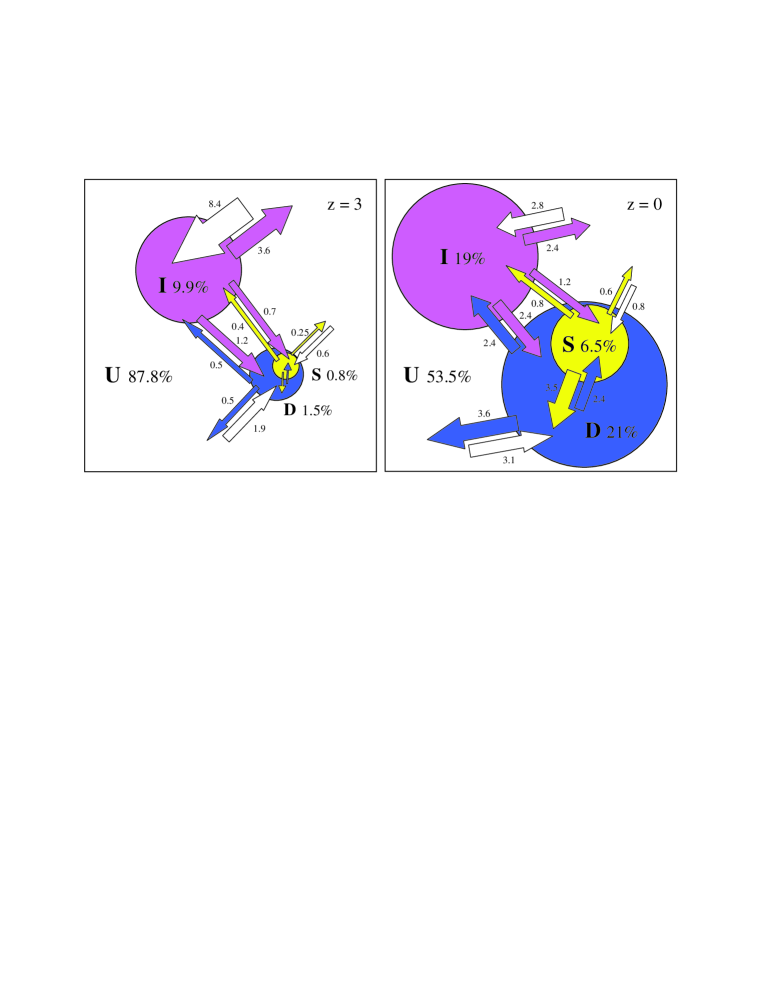
Figure 2: Mass distribution among the four components and exchange rates. U=unvirialized background, I=isolated halos, D=diffuse in host halos, S=subhalos. Mean densities are quoted in percentiles (i.e., units of $10^{-2}\langle\rho\rangle$), and flows in $10^{-2}\langle\rho\rangle$ Gyr^-1. The areas are proportional to the mass in the corresponding component. The thickness of the arrows is monotonic with the flow. Left: $z=3$. Right: $z=0$.

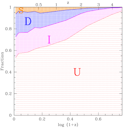
Figure 4: Fractional density of each one of the four components U,I,D,S (cf. Fig. 2) as function of redshift.

In presenting the exchange rates we can either focus on the origin of the incoming mass to each component or on the destiny of the outgoing mass from each component. The information content is redundant, because the $x$ origin of $y$ is the same as the $y$ destiny of $x$ in the previous time-step, but they allow two different angles of view. Figures 6 and 8 summarize the exchange rates in these two ways. They show the evolution of total mass density in each of the four components, and the flow rate into (from) each component from (into) each of the other components. We note that the general variation in time of many of the rates is slow. We fit this weak time dependence of the measured rates with a quadratic function in $\tilde{z}\equiv\log(1+z)$,

$$\log\dot{\rho}=\log(\dot{\rho}_{0})+b\tilde{z}+a\tilde{z}^{2}\,.$$ (2)

Table 1
Density fit coefficients ($\log{\rho_{0}}$),b,a∗
I	D	S	U
10.132	10.154	9.591	10.439
0.906	0.656	0.497	0.092
-2.287	-4.218	-3.220	-0.013
$\tilde{z}=\log(1+z)$
${}^{*}\log({\rho}_{x})=\log(\rho_{0})+b\tilde{z}+a\tilde{z}^{2}$
[${\rho}$]=h${}^{-1}M_{\odot}$(h-1Mpc)-3

We assign equal weights to the measured rates in the different time steps; this is under the assumption that the errors are dominated by cosmic variance, which we are not trying to model in detail. Table 1 displays the parameters for the quadratic functional fits to the density evolution of each component, $\rho(\tilde{z})$, the fits are accurate to $10-15\%$, and Table 2 displays the parameters for the functional fits to the whole matrix of flows, $\dot{\rho}_{xy}$. For example, from I to D, $\log\dot{\rho}_{ID}(\tilde{z})=9.306+0.043\tilde{z}-1.242\tilde{z}^{2}$, which equals 8.88 at $z=3$; thus $\dot{\rho}_{ID}=2.02\times 10^{9}$ at $z=0$ and $7.6\times 10^{8}$ at $z=3$, in units of $h^{-1}M_{\odot}(h^{-1}{\rm Mpc})^{-3}$ Gyr^-1. In general, the evolution slows down with time because of the $\Lambda$CDM cosmology; with $\Omega_{\rm m}=0.3$, the characteristic epoch for loitering is $z\sim 0.7$.

Table 2
Rate fit coefficients ($\log{\dot{\rho}_{0}}$),b,a∗
	I	D	S	U
		9.306	9.027	9.347
I	-	0.043	-0.872	-0.615
		-1.242	0.694	1.225
	9.367		9.305	9.408
D	-1.621	-	-1.673	-0.621
	0.776		-0.349	-1.212
	8.961	9.580		8.682
S	-1.589	-2.965	-	-0.462
	1.436	0.957		-0.258
	9.390	9.492	8.925
U	0.109	0.233	-0.842	-
	1.086	-1.277	0.830
$\tilde{z}=\log(1+z)$
${}^{*}\log({\dot{\rho}}_{xy})=\log(\dot{\rho}_{0})+b\tilde{z}+a\tilde{z}^{2}$
[${\dot{\rho}}$]=h${}^{-1}M_{\odot}$(h-1Mpc)-3Gyr-1

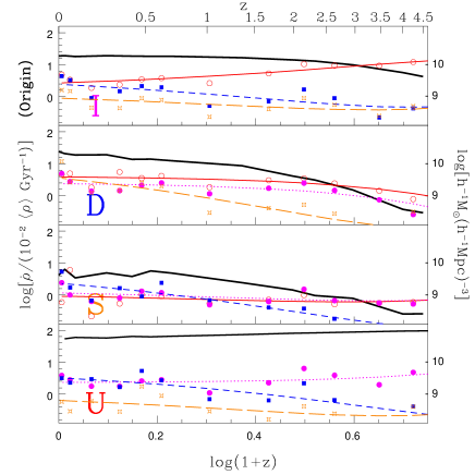
Figure 6: Time evolution of the mass density in each of the 4 components (thick black curve in each panel) in units of $h^{-1}M_{\odot}(\ h^{-1}{\rm Mpc})^{-3}$ (right axis) or equivalently $10^{-2}\times\langle\rho\rangle$, the comoving average density of the simulated cosmology (left axis, dropping the “Gyr^-1”). Also plotted are the incoming flow rate into each component from each of the other components (“Origin”) in units of $10^{-2}\times\langle\rho\rangle$Gyr^-1 (left axis). The symbols are the measured flow in the given time interval, and the curves are quadratic fits. Isolated halos I=filled circles, dotted lines, magenta; diffuse matter in host halos D=filled squares, short-dashed lines, blue; subhalos S=empty stars, long-dashed lines, orange; unvirialized matter U=open squares, solid lines, red.

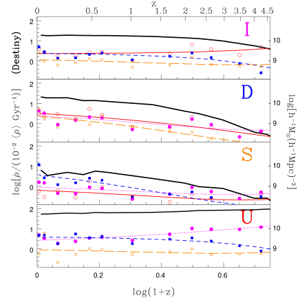
Figure 8: Destiny: same as Fig. 6, but showing the outgoing flow rate from each component into each of the other components.

3.1 Total mass distributions

The main features of the total mass evolution in each component in the redshift interval $z=4.5$ to 0 are as follows:

1. The isolated component, I, grows from 5 to 19, with most of the relative growth occurring at $z>2$.

2. The diffuse component, D, grows continuously from 0.2 to 19. The growth continues to be significant down to $z\sim 1$, long past the time when I component growth stagnates.

3. The subhalo component S grows at roughly a constant rate until $z\sim 1$, from 0.2 to 3.6, and then becomes rather constant.

4. The background U is depleted slowly, from a density of 87 before $z=3$ to 53 at $z=0$.

3.2 Origin and Destiny

The main characteristics of the origin of each component are as follows:

1. The origin of I (isolated halos) is dominated by accretion from U (unvirialized component) at a gradually decreasing rate, from 12 to 2.6 (recall that the flow units are $10^{-2}\langle\rho\rangle$Gyr^-1). About 100% of I is being added every Gyr at $z\sim 3$, while this fraction drops to $\sim 20\%$ at $z=0$. (Note also that $\sim$10% of I comes from D and S; this is mostly a consequence of small host halos turning into simple halos because of the disruption of all their subhalos).

2. The main source of D (diffuse matter in host halos) is accretion from U, at a slowly varying rate, from 1.1 to 3.6. In parallel, there is an important supply to D from infalling I, which is always about 1/3 of the total incoming flow. About 100% of D is being added every Gyr at $z\sim 2.5$, dropping to 40% at $z=0$. The expulsion rate from S into D, corresponding to the disruption of subhalos, grows continuously after $z\sim 3$, and becomes higher than the infall rate from I into D at $z<0.4$, and comparable to the accretion from U at $z=0$.

3. The origin of S at $z>1$ is divided about equally between I and U, at roughly a constant rate of $\sim 1$ each. At $z<1$, the origin of S becomes dominated by accretion from D, reaching a rate of 2.5 at $z=0$. The input to S is about 100% of S per Gyr at $z\sim 2.5$, and 70% after $z=2$. It is likely that fraction of the accretion to S from U is due to halos that formed outside of a host and subsequently fell in, however the time resolution of the simulation outputs analyzed did not allow the identification of the intermediate I component. The same applies to the fraction of matter that went to S through a D phase.

4. The little input to U comes mostly from expulsion of I, and at $z<0.5$ also from D, at the level of a few percent of U per Gyr.

The main features of the destiny of each component are as follows:

1. Isolated halos, I expel mass mostly into U, at roughly a constant rate of 2.5-3.5. I also turns into D at a growing rate that becomes comparable to 2.5 at $z<1$. The latter is likely due to I halos falling into groups and clusters and then being disrupted into D within a single timestep, without ever being identified as S subhalos. At $z\sim 4.5$, about 100% of I is being lost (to U) per Gyr, while after $z=2$ the outgoing rate (to U and D) is about a 1/3 of I. This is as expected from the relative masses of the isolated halos at the two redshifts [Sigad et al. (2000)], less concentrated density profiles at higher redshift [Bullock et al. (2000)], and a higher merger rate before $z\simeq 2$ [Kolatt et al. (1999)].

2. The diffuse component D outputs mass in roughly equal parts to U and I (the latter being mostly D+S turning into I). At $z<1$, a significant part of the outgoing mass goes also to S. The output rate from D to U grows from 0.3 to 3. The total output rate is about 250% of D per Gyr at $z\sim 4.5$, and about 1/3 of D after $z=2$.

3. The disruption of subhalos causes S to lose roughly a constant $\sim$40% of its total mass every Gyr to D, with a rate growing from 0.1 to 3. There is also some outflow from S to U at roughly a constant rate of 0.36-0.6, and transition from S to I at a rate 0.7-1.0.

4. The main destiny of U is I. The accretion from U to D becomes comparable after $z=1$, at a total accretion rate into halos of 6, which is $\sim 10\%$ of U per Gyr.

The largest absolute flow at $z>2$ is accretion from U to I, at a rate of $\sim 10$, partly balanced by a flow back from I to U at a rate of $\sim 4$. They reach a near balance by $z=0$, at a rate of $\sim 2.5$. At $z<1$, the dominant flow is the accretion from U to D, at a rate of $\sim 4$, which is approaching a balance with the back-flow from D to U only near $z=0$.

At $z>2$, all the halo components (especially I and D) absorb mass at a relative rate comparable to their own mass every Gyr, and lose mass at a lower rate. At $z<2$ the fractional mass inflow is typically 10 to 50% of each halo component per Gyr, and the outflow rate is only slightly lower. The S component exchanges mass at a high rate of 40-70% of its own mass every Gyr.

3.3 Net mass exchange rates

The evolution of the net  mass transfer rate between every two components ($\dot{\rho}_{xy}-\dot{\rho}_{yx}$) is shown in Fig. 10. Of course, the net transfer can be very different from the actual flows in each of the opposite directions. For example, when the flows in the opposite directions are equal, the net transfer is zero even when the entire population of each component has been exchanged. The main lessons from the net transfer rates are as follows:

1. The net exchange U-I at high $z$ is dominated by the accretion from U to I; it slows down in time while the expulsion from I to U increases. At $z\simeq 0.3$ the backflow becomes comparable to the build-up of I from U.

2. The net flows from U to S and from I to S are pretty constant at $\sim 0.25-0.35$.

3. There is always a significant net flow from U to D, at the level of $\sim 1$. It exceeds the net flow from U to I at $z\leq 1$. At $z<0.5$, the evaporation of D to U competes effectively with the slowly increasing accretion from U to D, resulting in the decreasing net flow.

4. The net flow from I to D starts low at early times due to the near absence of D material at $z>3.5$. It increases gradually until $z\simeq 0.5$ by the clustering of I accompanied by tidal stripping. At lower $z$ the signal is dominated by artificial fluctuations.

5. The net exchange between D and S is very low at $z>1$, where the accretion from D to S is only slightly higher than the tidal stripping from S to D. At later epochs, the tidal stripping becomes dominant causing the net exchange to reverse its sign and grow to $\sim 1$ at $z=0$.

In summary, we have presented the mass exchange rates between several components of cosmological matter in our simulations. We confirm the generally expected trend that the mass fraction of “unvirialized” background material (i.e., all mass outside of any identified halo) falls steadily as a function of time, directly or indirectly fueling the mass accumulation in isolated halos, subhalos, and the diffuse media of host halos. Although the flow of mass is dominated by the accumulation of unvirialized background material into and onto isolated halos and host halos, we find that there is a significant amount of mass loss from halos back to the unvirialized component and to the diffuse component of large host halos. In the next section we explore one possible implication of our derived mass exchange rates.

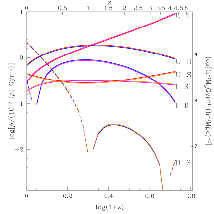
Figure 10: Net exchange rate between every two levels (x,y), i.e., $X-Y=\dot{\rho}_{xy}-\dot{\rho}_{yx}$, as calculated from the fits of Table $2$. Solid segments are for positive exchange rate while dashed segments represent redshift zones where $\dot{\rho}_{xy}<\dot{\rho}_{yx}$.

4 Integrated History: Metallicity

4.1 Model Predictions

Interesting astrophysical implications may be extracted from the integrated history of the mass in the different components. As an example, we describe an attempt to learn about the possible role of gravitational effects in determining the metallicity of the gas in the different components. We make the crude assumption that the baryons trace the mass distribution everywhere and at all times, and that the star formation rate per unit mass and the resulting metallicity yield are the same in all galactic halos at all times. This is based on a scenario in which supernova-driven winds are sufficiently energetic to drive the gas out of the galactic disks and distribute it in quasi-static equilibrium in the galactic halos (e.g., [Mac Low & Ferrara (1999)]), but that this feedback is not strong enough to drive the processed material out of galactic halos (e.g., [Vader (1986), Ferrara et al. (2000)]). The hypothesis we try to evaluate is that gravitational interaction is sufficient to strip the enriched matter from galactic halos and distribute it in the diffuse components [David et al. (1991), Gnedin (1998)].

This is of course an extreme hypothesis. Because star formation rates grow with the baryon density, the baryons that become stars are highly concentrated due to gas cooling in the centers of halos; and supernova-driven winds may not be able to distribute the metals produced by those stars throughout the halos. Doubtless in the real universe there is a mixture of the purely gravitational processes considered here, on the one hand, and the effects of baryonic physics (gas cooling, star formation, supernovae), on the other. In order to estimate the relative importance of gravitational vs. baryonic processes, however, it is simplest to consider extreme cases first.

Based on these simplifying assumptions, we virtually assign a fixed fraction of gas to each mass particle of the simulation, and associate with it a metallicity which grows in time in proportion to the time the particle has spent in a galactic halo. As defined above, the galactic halos are all of the subhalos plus all of the isolated halos.

We focus first on the diffuse component in host halos (D). We identify host halos more massive than $10^{13.6}h^{-1}M_{\odot}=4\times 10^{13}h^{-1}M_{\odot}$ with “clusters”, and those in the range $10^{12}-10^{13.6}h^{-1}M_{\odot}$ with “groups”. Although we use the term “groups” for this second component, these objects, especially those in the lower half of the mass range. are probably better associated with massive galaxies hosting satellites than the halos of what are typically referred to as galaxy groups. This should be kept in mind when comparing our predictions to observations, as discussed in §4.2.

For each host halo, we keep track of the fraction of the diffuse mass that spent less than a given amount of time in galactic halos. These fractions are averaged over all the host halos of each of the two mass classes. Fig. 12 shows the average time distributions at two different epochs. At $z=0.7$, when the $\Lambda$CDM universe considered here had an age of $\sim 7$ Gyr, the time distributions for the two mass classes are very similar; about half of the diffuse component has not spent any time in galaxies, namely it has been accreted directly from the unvirialized background. About 5% has spent more than 4.5 Gyr (similar to the solar age) inside galaxies. At $z=0$, the distributions become quite different. First, while for the massive hosts the fraction of D material that has not spent any time in galaxies is still $\sim 50\%$, this fraction is only $\sim 20\%$ for the less massive hosts. Second, while the D faction of massive hosts that has spent more than 4.5 Gyr inside galaxies is $\sim 10\%$, the corresponding fraction of less massive hosts is $\sim 60\%$. Thus, the diffuse component in “clusters” has not been enriched significantly by processed material since $z=0.7$, while in “groups” it has been enriched significantly during this recent epoch. This difference hints at a different metallicity enrichment history in clusters versus groups.

Figure 12: The distribution of time spent by the diffuse components in “galaxies”, at $z=0$ (thin) and $z=0.7$ (thick). The host halos are divided by mass into “clusters” and “groups”.

Figure 14 shows the overall metallicity production rate in our scheme as a function of redshift. This is estimated as the time derivative of the average metallicity, mass weighted in all halos. The general behavior of the metal production rate is a rise of about an order of magnitude between $z\simeq 4$ to $z\simeq 1-1.5$, followed by a gentler decline of about a factor of $3$ to the rate value at $z=0$. The interpretation of such a trend in light of observations will be further discussed in the last section (§5).

Figure 14: Metallicity production rate versus redshift. The symbols represent time derivatives of the halo mass weighted metallicities while the solid line is a parabolic fit to the equally weighted points (relative units).

Next, we consider the integrated metallicity in the different components defined above: the galactic halos I and S, the diffuse component D divided by host-halo mass into “clusters” and “groups”, and U, the unvirialized IGM. Since the absolute values of the yield and the gas fraction are unknown, we focus on the measurement of relative abundances, between different epochs or different environments. Figure 16 shows the computed evolution of metallicity $Z_{x}$ in each of these components, in units of the metallicity in clusters at $z=0$, $Z_{\rm cl}(0)$.

The average metallicity values of the different virialized components grow roughly in proportion to time for $z\sim 4$. In more detail, they all grow between $z=4$ and $2$ at a similar rate of about $\Delta Z/Z_{\rm cl}(0)=0.08\,{\rm Gyr}^{-1}$. After $z\simeq 2$ (namely, during the last 10 Gyr), the growth rate in clusters continues at a similar pace, but the growth rate in the other components speeds up somewhat, to $\Delta Z/Z_{\rm cl}(0)=0.17,0.20,0.24{\rm Gyr}^{-1}$ for the diffuse component in groups, field galaxies (I), and clustered galaxies (S) respectively.

The average metallicity in the diffuse component in clusters and groups (D) is about one half that in the galaxies (I and S). This is in agreement with our finding in § 3 that the (enriched) flow from I and S to D is roughly comparable to the (fresh) flow from U to D.

The metallicity in clustered galaxies (S) is higher than that of field galaxies (I), by about one third. This is because most S halos are old; they formed early as I halos, then fell into groups and clusters, and thus typically had a long time to produce metals. Many of the current I halos are relatively young, and therefore less metal rich.

The faster growth rate in groups versus clusters at $z<2$ leads to a present metallicity in groups almost twice the metallicity in clusters. This is in general agreement with the difference in the time distribution seen in Fig. 12.

The average metallicity in the unvirialized (U) background is roughly constant since $z\sim 4$, at a level of $Z_{\rm IGM}/Z_{\rm cl}(0)\simeq 10^{-4}-10^{-3}$.

4.2 Comparison with observations

In order to compare our predictions with observations we have to consider in some more detail the association of the simulated halo components with observed objects. The association of the most massive host halos with galaxy clusters is natural at all redshifts. At low redshift, the low mass range of host halos fits well the mass range of galaxy groups [Hwang et al. (1999), Davis et al. (1999)] or even massive galaxies with satellite companions. It is less obvious what observations to associate with the low mass host halos at high redshift. The choice might be damped Ly$\alpha$ systems (DLAS), or even Lyman-limit systems and high column density ($\sim 10^{17}$cm^-2) Lyman-forest clouds. At high redshift, the unvirialized IGM can be identified with Ly$\alpha$ systems of very low column densities, $\sim 10^{14}$cm^-2, which are shown by simulations ([Davé et al. (1998), Lu et al. (1998)]) to correspond to the mean mass density at that time.

For clusters today the observational estimate is $\bar{Z}_{\rm cl}(0)=(0.29\pm 0.01)Z_{\odot}$, with a relatively small true intrinsic variance between clusters of order $0.06Z_{\odot}$ [Edge & Stewart (1991), Yamashita (1992)]. We show in Fig. 16 three data points with error bars based on measurements of Fe relative abundance by ?) (at ${\bar{z}}\simeq 0.2,0.4$), and ?) (at ${\bar{z}}\simeq 0.8$). Thus, the observed metallicity in the diffuse component of clusters does not seem to vary significantly between $z=0$ and 0.4, and not to change by more than a factor of two out to $z\sim 0.8$. This is in agreement with the model predictions. An even weaker evolution rate is predicted by our model for the most massive clusters in the simulation, $M>10^{14}h^{-1}M_{\odot}$ (not shown in the figure); this improves the agreement with the observations, for which massive clusters were preferentially selected, especially at high redshift.

The observational estimates of the $z=0$ metallicity in groups and massive galaxies with satellites are less secure, and one cannot yet confirm or refute the predicted trend of $Z_{\rm gr}(0)\sim 1.8Z_{\rm cl}(0)\sim 0.5Z_{\odot}$. The average metallicity of the diffuse component in rich galaxy groups is measured locally to be $\bar{Z}_{\rm gr}(0)\simeq 0.35Z_{\odot}$ [Hwang et al. (1999)] with the scatter being dominated by an intrinsic variance between groups of at least $0.1$, partly due to Poisson noise and the small number of galaxies per group. ?) studied 17 poor groups and found metallicities of $\sim 0.1Z_{\odot}$ for $0.7-1$ keV groups ($\sim 5-8\times 10^{13}h^{-1}M_{\odot}$) and $\sim 0.2-0.5Z_{\odot}$ for more massive groups. These values are smaller than our results.

However recently ?) showed that for $12$ bright groups, much higher metallicities are obtained if two-temperature models are applied with or without cooling flows. The group metallicities increased from ${\bar{Z}}_{\rm gr}=0.29Z_{\odot}$ using a single temperature model to $0.65-0.75Z_{\odot}$ depending on the details of the two temperature models. These values are much more consistent with the values presented here. Perhaps, though, a better comparison with our small-mass hosts is the metallicity estimates of hot gas in massive elliptical galaxies at $z=0$. The measured values [Matsumoto et al. (1997), Buote & Fabian (1998)] range all the way from ${\bar{Z}}=(0.19\pm 0.12)Z_{\odot}$ (when single-temperature models are invoked) through ${\bar{Z}}=(0.6\pm 0.5)Z_{\odot}$ (when better fits of two-temperature models are considered), and up to ${\bar{Z}}=0.9Z_{\odot}$ for the galaxies of best signal-to-noise ratio [Buote & Fabian (1998)]. The estimate for the metallicity of the Galactic halo interstellar gas, however is lower [Savage & Sembach (1996)] and stands on about $0.1$ solar for most elements. The observed metallicities would be consistent with our predictions for ${\bar{Z}}_{\rm gr}(0)/{\bar{Z}}_{\rm cl}(0)$ if a substantial fraction of the less massive host halos which we classified as “groups” actually correspond to the massive galaxies of $Z\sim 0.6-0.9Z_{\odot}$.

If DLAS are the counterparts of our “group” halos at high redshift, then the relevant metallicity measurements [Lu et al. (1996), Prochaska & Wolfe (1999)] give ${\bar{Z}}_{\rm DLA}\simeq 0.07Z_{\odot}$ at $z\mathrel{\mathchoice{\vbox{\offinterlineskip\halign{\hfil$\reset@font\displaystyle#$\hfil\cr>\cr\sim\cr}}}{\vbox{\offinterlineskip\halign{\hfil$\reset@font\textstyle#$\hfil\cr>\cr\sim\cr}}}{\vbox{\offinterlineskip\halign{\hfil$\reset@font\scriptstyle#$\hfil\cr>\cr\sim\cr}}}{\vbox{\offinterlineskip\halign{\hfil$\reset@font\scriptscriptstyle#$\hfil\cr>\cr\sim\cr}}}}1.5$. The measurement for a sample of DLAS with $z\mathrel{\mathchoice{\vbox{\offinterlineskip\halign{\hfil$\reset@font\displaystyle#$\hfil\cr<\cr\sim\cr}}}{\vbox{\offinterlineskip\halign{\hfil$\reset@font\textstyle#$\hfil\cr<\cr\sim\cr}}}{\vbox{\offinterlineskip\halign{\hfil$\reset@font\scriptstyle#$\hfil\cr<\cr\sim\cr}}}{\vbox{\offinterlineskip\halign{\hfil$\reset@font\scriptscriptstyle#$\hfil\cr<\cr\sim\cr}}}}1.5$ [Pettini et al. (1999)] is ${\bar{Z}}\simeq 0.1Z_{\odot}$. These data points are shown in Fig. 16. When compared to today’s cluster metallicity, the observed values correspond to $\bar{Z}_{\rm gr}(z\sim 1.5)/\bar{Z}_{\rm cl}(0)\sim 0.2$, in surprisingly good agreement with the model predictions. If, alternatively, we associate DLAS at high $z$ with groups and very massive galaxies with satellites at $z=0$ (both have similar hydrogen column densities in the range $10^{20}-10^{21}$ atoms cm^-2), we obtain a ratio $\bar{Z}_{\rm gr}(z\sim 1.5)/\bar{Z}_{\rm gr}(0)\sim 0.26$, also in agreement with the model predictions. However, there are certain caveats associated with this comparison. For example, unlike the measurements in groups at $z=0$, the observed metallicities at high $z$ were not evaluated by Fe abundance. Also, these abundances refer in large to the cold gas component, and are relevant to our model predictions only if the assumption of proper mixing between the cold disk and the hot halo is valid. Finally, the large scatter in these measurements at high $z$ weakens any conclusion drawn on the basis of the mean values.

The predicted metallicity of the unvirialized IGM may be compared to the very low column density Ly$\alpha$ clouds. Data for abundances of these exist only for $z\simeq 2.2-4$ [Savaglio (1997), Davé et al. (1998), Lu et al. (1998)]. These results show metallicities in the range $0.3-3\times 10^{-4}$. Since no significant systematic evolution in metallicity is observed in this redshift range, these values may be indicative of lower redshift values as well. The simulation analysis shows little evolution in the metallicity of the U component, and fluctuations in the range $Z_{\rm IGM}=0.3-1\times 10^{-3}Z_{\rm cl}(0)\sim 1-3\times 10^{-4}Z_{\odot}$. This agrees well with the observed values.

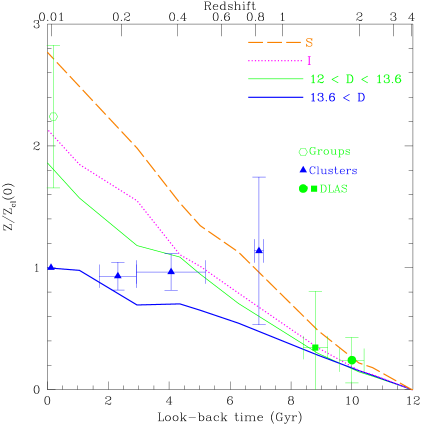
Figure 16: Metallicity of the different components as function of look-back time relative to the cluster metallicity at $z=0$. Here those halos whose mass lies between $10^{12}$ and $4\times 10^{13}h^{-1}M_{\odot}$ are called “groups,” (thin solid) while those with higher mass are called “clusters” (thick solid). The three data points for clusters are from the observed Fe abundance in clusters from Mushotzky & Loewenstein (1997) ($z\simeq 0.2$ and 0.4) and Donahue et al. (1999) ($z\simeq 0.8$). The data point for groups (empty hexagon) at $z=0$ (shifted for clarity) is from Buote (2000) cooling flow model. The two data points for DLAS at $z=1-2$ are from Prochaska & Wolfe (1998) (circle, higher $z$) and Pettini et al. (1999) (square, lower $z$). The IGM (U) component metallicity is not shown.

5 Conclusion and Discussion

We have learned that the role of gravity does not end when a virialized halo is formed. Gravity is responsible for a continuous and substantial exchange of matter among the different components of halos and diffuse media. This exchange may affect the formation and evolution of luminous galaxies inside the halos and their feedback into the environment. It should therefore be included in the modeling of structure formation. We have analyzed this exchange between 4 basic components of DM halos and diffuse media, and provided quantitative exchange rates to be used in further investigations. We then showed, in particular, that gravitational interaction and stripping may provide the mechanism which produces a significant part of the relatively high metallicities observed in the diffuse hot gas of big galaxies, groups and clusters as well as the unvirialized background IGM.

A summary of the matter division and exchange rates is as follows. Most of the mass within identified halos ($\mathrel{\mathchoice{\vbox{\offinterlineskip\halign{\hfil$\reset@font\displaystyle#$\hfil\cr>\cr\sim\cr}}}{\vbox{\offinterlineskip\halign{\hfil$\reset@font\textstyle#$\hfil\cr>\cr\sim\cr}}}{\vbox{\offinterlineskip\halign{\hfil$\reset@font\scriptstyle#$\hfil\cr>\cr\sim\cr}}}{\vbox{\offinterlineskip\halign{\hfil$\reset@font\scriptscriptstyle#$\hfil\cr>\cr\sim\cr}}}}10^{11}h^{-1}M_{\odot}$) is located in “isolated” galactic halos before $z\sim 2$. Then about 15% of their mass accumulates in groups and clusters per Gyr, while a similar fraction is expelled back to the unvirialized background. Subhalos tend to form later, mostly by a constant-rate accretion from outside the clusters, but at $z\leq 1$ they also accrete from the cluster diffuse medium. The subhalos are constantly disrupted such that about one half the subhalo mass is being exchanged every Gyr. The diffuse medium in clusters is built by accreting extra-cluster material, composed on average of 40% halos and 60% unvirialized matter. The disruption of subhalos becomes a significant source after $z\sim 0.5$. Finally, the unvirialized IGM is enriched mostly by mass loss from isolated galactic halos, and at late epochs, $z<1$, also by expulsion from clusters.

The results summarized above highlight important limitations of the recipes used by current semi-analytic models [Kauffmann et al. (1993), Cole et al. (1994), Somerville & Primack (1999)], and offer possible routes for improvement. In particular,

• Matter expulsion from isolated halos, which is found here to be quite significant, is completely ignored in the semi-analytic models because they are based on a hierarchical clustering formalism which does not take into account such a process. Tidal stripping and gravitational heating in collisions are known to be more effective in denser environments and at higher redshifts [Kolatt et al. (2000)]. While the time dependence can be incorporated in semi-analytic models quite straightforwardly, the environment dependence is harder to mimic.

• We notice that “fresh” matter from the unvirialized component (U) finds its way to subhalos (S), while current semi-analytic models stop the supply of DM and fresh gas to halos as soon as they are incorporated in bigger halos, even when the subhalo and the host are of comparable masses.

• We find that accretion from diffuse matter in halos (D) onto subhalos (S) becomes the main source of matter for S at low redshift, while this process is completely ignored in semi-analytic models. Some semi-analytic models do allow for tidal stripping of subhalos, but the matter exchange between subhalos and their hosts seems to be a two-way process that should be treated as such in the semi-analytic models.

• The fitting formulae Eq. (2) and Table 1 describing the exchange rates as a function of time can be used as a first attempt to improve semi-analytic treatment of matter exchange. Since we only provide average exchange rates without specifying their dependence on halo mass, a sensible utilization of these formulae is via the implied fractional exchange rates rather than the absolute rates.

A convenient use of these formulae may be a direct integration to yield the density of each component at an arbitrary time. Integrations of the rate equations in the redshift range of $[4-0]$ yield results accurate to about $20\%$ in comparison to the actual densities at the upper limit of the integration time. The initial conditions were taken to be the actual density of the relevant component at the lower limit of the integral (higher redshift). Both the upper and lower limits of the integrals can be read directly from Table $1$.

The second part of this paper is a more speculative attempt to demonstrate how the matter exchange may affect measurable quantities. This is an attempt to predict metallicities from simulations that do not include explicitly any gas, by simply assuming the metallicity of the different components is proportional to the time this matter spent in galactic halos. We effectively assume that supernova winds expel processed matter from the disk out into each halo, so that this processed matter spreads uniformly in it. However we assume that the SN winds are not powerful enough to drive the matter all the way out of individual halos. We address whether gravitational interactions could have acted to provide the missing energy and thus to enrich the IGM with this material. We avoided any calibration of the specific star formation rate and yield in absolute terms, and instead addressed relative metallicities, comparing different times or different environments.

We found that the relative metallicities, compared to that of galaxies, obtained by gravitational processes in the diffuse components of groups, clusters, and the IGM are in the same ball park as the observed metallicities at $z=0$. This scenario seems to predict an anti-correlation between the metallicity and the mass of the host halo, which is yet to be tested against observations. For example, it may be possible to measure halo masses at high z from line profiles [Prochaska & Wolfe (1997), Prochaska & Wolfe (1998), Haehnelt et al. (1997), Maller et al. (2000)] and thus allow a direct confrontation of prediction and observation. The predicted slow evolution of metallicity in clusters from $z=1$ to 0 is consistent with observations. Matching the simulated halos with real objects at high redshifts is more ambiguous; if DLAS or Ly$\alpha$ systems are the high-redshift counterparts of local groups and very massive galaxies with satellites, then the predictions agree with the observed metallicity evolution. Our tentative conclusion is that gravitational effects could indeed be largely responsible for bringing the metals from galactic halos into the diffuse media.

The process of a gravitational merger mechanism for gravitational enrichment has already been addressed by Gnedin (1998), in the context of interacting field galaxies and the IGM, using $\leq 3\ h^{-1}{\rm Mpc}$ simulations in which sub-cell physics was added “by hand”. Our N-body results in a cosmological volume confirm the feasibility of this general idea and demonstrate that gravity may be responsible for the redistribution of metals in the diffuse component of clusters and groups as well. The very low metallicity predicted by our analysis for the unvirialized IGM compared to the virialized components is in agreement with the predictions based on the abovementioned simulations.

A more elaborate model for the hot gas and metal redistribution in clusters, groups, and massive ellipticals [Mathews & Brighenti (1998), Brighenti & Mathews (1999a), Brighenti & Mathews (1999b)] have demonstrated some of the difficulties in combining a mixture of supernovae as the source of metals and enrichment of the diffuse media. While these models succeed in reproducing the observed abundances of hot gas in elliptical galaxies, the straight sum of the predicted enrichment from the member galaxies fails to account for the observed metallicity of the diffuse media in groups and clusters. However, close encounters of galactic halos and the associated harassment ([Moore et al. (1999)]) are more frequent in the crowded environment of groups and clusters [Kolatt et al. (2000)] and may thus provide the missing ingredient in these models.

While we mainly addressed the average metallicity in the different environments, the scatter about the mean may also be of interest. A large scatter in metallicity at a given density has been stressed by ?), but the mass bins used here can be more easily identified with real objects, and thus allow a more direct comparison with observations.

Of course, our attempt to estimate metallicities is extremely simplified and it ignores many complexities involving gas dynamics and feedback that should be properly addressed in more detailed studies.

For example, the gas cannot be uniform and cannot trace perfectly the dark-matter distribution. The cooling time is in fact different at different positions in the halo and at different times, and it is likely to develop the two phases of cold clouds in a hot medium. The feedback may not be strong and persistent enough to keep the expelled gas hot and transported to large radii in the galactic halos, where most of the stripping is expected to occur.

In reality, the metallicity yield must vary in time and in space. A specific worry is associated with the fact that the star-formation rate (SFR) is known to drop at late epochs, $z<1$ [Madau et al. (1997), Somerville et al. (2000)]. This is largely a result of the gas processes, such as cooling, that determine the characteristic upper limit of galactic masses, which we do not explicitly simulate. Furthermore, we do not explicitly take into account the effect of gas depletion in old halos on the SFR. Two features of our analysis ease this problem. First, our analysis does mimic a moderate drop in the SFR at late times, if SFR is taken to be the net flow rate (time derivative of the density) to each galactic component. This drop is due to the combination of three effects: (a) the slow down in the growth of fluctuations due to the $\Lambda$CDM cosmology, (b) the imposed minimum on the halo masses, and (c) the identification of only simple halos with galactic halos. Second, the yield of metals is expected to vary slower than the SFR because it results from stars of different ages.

A related, interesting comparison to observations can be made by the examination of the overall metallicity production rate in view of the SFR diagrams as obtained from observations (the “Madau diagrams”). A direct comparison between the metallicity production rate in our recipe (Fig. 14) and recent versions of SFR diagrams (see Somerville et al. 2000 for references) indicate two distinct differences: (i) The SFR peak is obtained at a higher redshift ($z\simeq 2.5-3$) than in our recipe for the metal production ($z\simeq 1-2$) (ii) the drop from the SFR peak value to its $z=0$ value is slightly bigger ($\sim 3-4$) than our value ($\sim 2-3$). However the link between an SFR diagram and metallicity production diagrams involves the assumption that all metals are produced by type II supernovae which closely trace the SFR. If in contrast, a large fraction of metals (especially Iron, from which the cluster metallicity is calculated) is produced in type Ia supernovae then the one to one mapping between SFR and metallicity production becomes less clear. Such SNIa contribution to the metal production is now favored by observations (cf. [Renzini (2000)]). In a scenario where combined contributions from different SN types dictate the metallicity production rate, the observational SFR diagrams can be easily reconciled with the metallicity production rate as derived by the proposed recipe of this paper.

Our comparison with metallicity observations is also very simplified. For example, our simple model provides the volume-average metallicity within the host halos, but in reality one may expect spatial gradients in metallicity. The observations, which are sometimes directed to different positions in the halos, e.g., to cluster centers, may therefore yield different metallicities. Another complication is that the metals may be shared between (at least) two phases of gas, cold and hot, as well as the stellar and dust components.

Our crude treatment of one single “metallicity” is an over-simplification, because actual metallicity measurements refer to a variety of elements, usually different elements at different redshifts depending on the detectability of the corresponding spectral lines. Moreover, since different elements in different abundances are produced through a variety of mechanisms [Mathews & Brighenti (1998), Brighenti & Mathews (1999a), Brighenti & Mathews (1999b)], the detailed history of various processes may be relevant for the metal production. A similar difficulty arises due to the (sometimes unknown) ionization state of the medium in which metallicities are observed, because in our simple model we cannot determine the gas temperature.

Our metallicity estimates should therefore be considered very crude and serve only as an encouraging indication for the possible important role of gravity in the large-scale exchange of metals.

It will be very interesting to see how important “nature” (dark matter physics) is compared to “nurture” (baryonic physics). The fact that the Madau-like plot (Figure 14), based on including only gravitational effects, looks reasonably similar to the observationally based plot is encouraging. Semi-analytic modelers should accept the challenge to disentangle the relative roles of “nature” vs. “nurture.”

References

- Amram et al. (1994) Amram P., Marcelin M., Balkowski C., Cayatte V., Sullivan W. T., Le Coarer E., 1994, AAPS, 103, 5
- Barnes & Hernquist (1992) Barnes J. E., Hernquist L., 1992, ARA&A, 30, 705
- Brighenti & Mathews (1999a) Brighenti F., Mathews W. G., 1999a, ApJ, 515, 542
- Brighenti & Mathews (1999b) Brighenti F., Mathews W. G., 1999b, ApJ, 512, 65
- Bryan & Norman (1998) Bryan G., Norman M., 1998, ApJ, 495, 80
- Bullock (1999) Bullock J., 1999, Ph.D. thesis, University of California, Santa Cruz
- Bullock et al. (2000) Bullock J., Kolatt T., Sigad Y., Primack J., Dekel A., Kravtsov A., Klypin A., 2000, MNRAS, in press (BKS+)
- Buote (2000) Buote D. A., 2000, MNRAS, 311, 176
- Buote & Fabian (1998) Buote D. A., Fabian A. C., 1998, MNRAS, 296, 977
- Cen & Ostriker (1999) Cen R., Ostriker J., 1999, ApJ, astro-ph/9903207
- Cole et al. (1994) Cole S., Aragón-Salamanca A., Frenk C., Navarro J., Zepf S., 1994, MNRAS, 271, 781
- Davé et al. (1998) Davé R., Hellsten U., Hernquist L., Katz N., Weinberg D. H., 1998, ApJ, 509, 661
- David et al. (1991) David L. P., Forman W., Jones C., 1991, ApJ, 380, 39
- Davis et al. (1999) Davis D. S., Mulchaey J. S., Mushotzky R. F., 1999, ApJ, 511, 34
- Donahue & et al. (2000) Donahue , et al. , 2000, ApJ, submitted
- Edge & Stewart (1991) Edge A. C., Stewart G. C., 1991, MNRAS, 252, 428
- Fabian (1994) Fabian A. C., 1994, ARA&A, 32, 277
- Fabian & Nulsen (1994) Fabian A. C., Nulsen P. E. J., 1994, MNRAS, 269, L33
- Ferrara et al. (2000) Ferrara A., Pettini M., Shechekinov Y., 2000, MNRAS, in press, astro-ph/0004349
- Gnedin (1998) Gnedin N. Y., 1998, MNRAS, 294, 407
- Haehnelt et al. (1997) Haehnelt M., Steinmetz M., Rauch M., 1997, ApJ, 495, 64
- Hwang et al. (1999) Hwang U., Mushotzky R., Burns J., Fukazawa Y., White R., 1999, ApJ, 516, 604
- Kauffmann et al. (1993) Kauffmann G., White S., Guiderdoni B., 1993, MNRAS, 264, 201
- Klypin et al. (1999) Klypin A., Gottlöber S., Kravtsov A., Khokhlov A., 1999, ApJ, 516, 530
- Kolatt et al. (2000) Kolatt T., Bullock J., Sigad Y., Primack J., Dekel A., Kravtsov A., Klypin A., 2000, MNRAS
- Kolatt et al. (1999) Kolatt T. et al., 1999, ApJ, 523, L109
- Kravtsov et al. (1997) Kravtsov A. V., Klypin A. A., Khokhlov A. M., 1997, ApJS, 111, 73
- Lacey & Cole (1993) Lacey C., Cole S., 1993, MNRAS, 262, 627
- Lacey & Cole (1994) Lacey C., Cole S., 1994, MNRAS, 271, 676
- Lu et al. (1996) Lu L., Sargent W., Barlow T., Churchill C., Vogt S., 1996, ApJS, 107, 475
- Lu et al. (1998) Lu L., Sargent W., Barlow T., Rauch M., 1998, preprint, astro-ph/9802189
- Mac Low & Ferrara (1999) Mac Low M.-M., Ferrara A., 1999, ApJ, 513, 142
- Madau et al. (1997) Madau P., Pozzetti L., Dickinson M., 1997, ApJ, 498, 106
- Maller et al. (2000) Maller A., Prochaska J., Somerville R., Primack J., 2000, MNRAS, submitted
- Mathews & Brighenti (1998) Mathews W. G., Brighenti F., 1998, ApJ, 503, L15
- Matsumoto et al. (1997) Matsumoto H., Koyama K., Awaki H., Tsuru T., Loewenstein M., Matsushita K., 1997, ApJ, 482, 133
- Moore et al. (1999) Moore B., Lake G., Quinn T., Stadel J., 1999, MNRAS, 304, 465
- Mushotzky & Loewenstein (1997) Mushotzky R., Loewenstein M., 1997, ApJ, 481
- Natarajan et al. (1998) Natarajan P., Kneib J. P., Smail I., Ellis R. S., 1998, ApJ, 499, 600
- Navarro et al. (1995) Navarro J., Frenk C., White S., 1995, MNRAS, 275, 56
- Pettini et al. (1999) Pettini M., Ellison S. L., Steidel C. C., Bowen D. V., 1999, ApJ, 510, 576
- Press & Schechter (1974) Press W. H., Schechter P., 1974, ApJ, 187, 425
- Prochaska & Wolfe (1999) Prochaska J. X., Wolfe A., 1999, ApJS, 121, 369
- Prochaska & Wolfe (1997) Prochaska J. X., Wolfe A. M., 1997, ApJ, 487, 73
- Prochaska & Wolfe (1998) Prochaska J. X., Wolfe A. M., 1998, ApJ, 507, 113
- Renzini (2000) Renzini A., 2000, in Walsh J., Rosa M., ed, Chemical evolution from zero to high redshift, Springer, Berlin, astro-ph/9902361
- Savage & Sembach (1996) Savage B. D., Sembach K. R., 1996, ApJ, 470, 893
- Savaglio (1997) Savaglio S., 1997, in P. Petitjean S. C., ed, IAP colloquium: Structure and Evolution of the IGM from QSO Absorption Lines
- Sigad et al. (2000) Sigad Y., Kolatt T., Bullock J., Dekel A., Primack J., Kravtsov A., Klypin A., 2000, MNRAS, submitted
- Somerville & Primack (1999) Somerville R., Primack J., 1999, MNRAS, 310, 108
- Somerville et al. (2000) Somerville R., Primack J., Faber S., 2000, MNRAS, in press, astro-ph/0006364
- Tyson et al. (1998) Tyson J. A., Kochanski G. P., Dell’Antonio I. P., 1998, ApJ, 498, L107
- Vader (1986) Vader J. P., 1986, ApJ, 305, 669
- Yamashita (1992) Yamashita K., 1992, in Tanaka Y., Koyama K., ed, Frontiers of X-ray Astronomy. Tokyo: Universal Academy Press