The Friedmann-Lemaître models in perspective

Abstract

I show that all FRW models (four dimensional pseudo-Riemannian manifolds with maximally symmetric space) can be embedded in a flat Minkowski manifold with 5 dimensions. The pseudo Riemannian metric of space-time  is induced by the flat metric. This generalizes the usual embedding widely used for the de Sitter models. I give the coordinate transformations for the embedding. Taking into account the spatial isotropy, one can reduce space-time to a two-dimensional surface, embedded in a three-dimensional Minkowski space. This allows to give exact graphic representations of the FRW models, and in particular of their curvature.

1 Introduction

Although immediate experience indicates that our space-time has four dimensions, modern physics evocates additional dimensions in various occasions. Gauge theories involve (principal) fiber bundles where the fibers may be seen as additional (internal) dimensions where the gauge fields live, usually not considered as physical, since they do not mix with the space-time  dimensions. However, the simplest gauge theory, namely the electromagnetism, has been tentatively described by a five dimensional theory (Kaluza, Kaluza (1921); Klein, 1926, (1927); Thiry, Thiry (1947)). It is not clear, in this case, that the 5 th dimension may be seen as a physical one, but Souriau (Souriau (1963)) has proposed a genuine 5 dimensional theory of this type.

More recently, string theories, M-theory, branes are formulated in a multidimensional space-time. Although most often compactified, the additional dimensions are considered as physical, in the sense that some interactions are able to propagate through them.

An appealing property of the Kaluza – Klein theories is the fact that the five-dimensional space-time, in which the Einstein equations are solved, is Ricci flat (and thus devoid of matter), although the embedded 4 dimensional manifold  corresponding to space-time, our world, is curved according to the four-dimensional Einstein equations with sources.

In this paper, I show that all the Friedmann-Robertson-Walker cosmological models can be embedded in a flat (Minkowskian) five-dimensional space-time ${\cal M}_{5}$. Such an embedding is known for a long time for the de Sitter space-time, which appears so as an hyperboloid ${\cal H}$ in ${\cal M}_{5}$. This embedding is widely used, mainly for pedagogical and illustrative purposes (see, e.g., Hawking and Ellis Hawking (1973)), and presents interesting properties for cosmological calculations. Recently, it has for instance been used to explore the quantification on de Sitter space-time (Bertola et al., Bertola (2000)). Also it is well known that a three dimensional space with maximal symmetry can be embedded in a flat Euclidean or Lorentzian manifold, also allowing interesting possibilities for calculations (see, e.g., Triay et al., Triay (1996)).

This work can be seen as a generalization of such embeddings to space-times with less symmetries (in fact with maximal spatial symmetry only). All embeddings are in a flat five-dimensional space ${\cal M}_{5}$ with Lorentzian signature (because of this signature, a flat space does not appear as a plane, as can be seen below). This generalizes also some work made by Wesson (Wesson (1994)) for some peculiar big bang models. The potential applications are the same than for the de Sitter case. First, this allows to visualize the arbitrary and varying curvature of space-time, in the same way that de Sitter space-time is visualized under the form of a hyperboloid embedded in ${\cal M}_{5}$. I emphasize that this makes the space-time curvature visible, not only its spatial part (which is very simple in all cases, of the three well known types, flat, spherical or hyperbolic), the temporal part being not given by the curve $R(t)$. In Section 2, I give explicitly the embedding formulae for an arbitrary space-time  with maximal spatial curvature, distinguishing three cases according to its sign. In Section 3, I consider the cosmic dynamics which, by the Friedmann equations, restricts the geometrical possibilities. I consider in more details some cosmological models.

2 Cosmology in 5 dimensions

I recall the metric of a Friedmann-Robertson-Walker model ${\cal M}_{k}$ ,

$$g_{AB}=dt^{2}-R(t)^{2}\leavevmode\nobreak\ d\sigma_{k}^{2},\leavevmode\nobreak\ \leavevmode\nobreak\ \leavevmode\nobreak\ \leavevmode\nobreak\ \leavevmode\nobreak\ \leavevmode\nobreak\ \leavevmode\nobreak\ \leavevmode\nobreak\ \leavevmode\nobreak\ \leavevmode\nobreak\ A,B=0,1,2,3$$

where $d\sigma_{k}^{2}$ is the metric of a maximally symmetric 3-d space with curvature $k=-1,0,1$,

$$d\sigma_{k}^{2}=d\chi^{2}+S_{k}^{2}(\chi)\leavevmode\nobreak\ d\omega^{2},$$

where $S_{-1}(\chi):=\sinh\chi$, $S_{0}(\chi):=\chi$, $S_{1}(\chi):=\sin\chi$. The function $R(t)$ is given by the dynamics (see 3). In this section, it will remain arbitrary, so that the geometrical embedding appears very general.

I call ${\cal M}_{5}$ the Minkowski space-time in five dimensions with the flat metric

$$ds^{2}=\eta_{\mu\nu}\leavevmode\nobreak\ dx^{\mu}\leavevmode\nobreak\ dx^{\nu},\leavevmode\nobreak\ \mu,\nu=0,1,2,3,4.$$ (1)

I will show that every Friedmann-Lemaître model can be seen as a four dimensional submanifold (hypersurface) of ${\cal M}_{5}$.

In the Friedmann-Lemaître models, space has maximal symmetry and is, in particular, isotropic. This isotropy is expressed by the action of the group SO(3) of the spatial rotations $R^{+}(\theta,\phi)$, which coincides with the subgroup $G_{(123)}$ of rotations in the three-dimensional subspace ${\cal M}_{3}$ of ${\cal M}_{5}$ described by the coordinates $x^{1},x^{2},x^{3}$. Thus, any point of ${\cal M}_{k}$ may be written

$$(x^{0},x^{1},x^{2},x^{3},x^{4})=R^{+}(\theta,\phi)\leavevmode\nobreak\ (x^{0},y,0,0,x^{4}),$$

so that

$$x^{1}=y\leavevmode\nobreak\ \cos\phi,$$

$$x^{2}=y\leavevmode\nobreak\ \sin\phi\leavevmode\nobreak\ \cos\theta,$$

and

$$x^{3}=y\leavevmode\nobreak\ \sin\phi\leavevmode\nobreak\ \sin\theta.$$

Thus, in the following, I will simply consider the three dimensional flat manifold ${\cal M}_{3}$ as embedding space, with the three coordinates $x^{0},x^{1}=y$ and $x^{4}$ (putting $\phi=\theta=0$), since the others can be trivially reconstructed by action of the spatial rotations. Thus, any point in ${\cal M}_{3}$ represents a two-sphere in ${\cal M}_{5}$. Space and time are measured in arbitrary identical units (I impose $c=1$). In the next sections, I will use $H_{0}^{-1}$, the Hubble time, as a common unit.

2.1 Negative curvature :

I consider ${\cal M}_{-}$ defined parametrically in ${\cal M}_{5}$ through the equations

$$x^{0}=R(t)\leavevmode\nobreak\ \cosh\chi$$ (2)

$$x^{1}=R(t)\leavevmode\nobreak\ \sinh\chi\leavevmode\nobreak\ \cos\phi$$

$$x^{2}=R(t)\leavevmode\nobreak\ \sinh\chi\leavevmode\nobreak\ \sin\phi\leavevmode\nobreak\ \cos\theta$$

$$x^{3}=R(t)\leavevmode\nobreak\ \sinh\chi\leavevmode\nobreak\ \sin\phi\leavevmode\nobreak\ \sin\theta$$

$$x^{4}=\int^{t}dt^{\prime}\leavevmode\nobreak\ \sqrt{\dot{R}^{2}-1}.$$

In this case, I have written explicitly the five equations to give insights to the geometry. In ${\cal M}_{3}$, they reduce to

$$x^{0}=R(t)\leavevmode\nobreak\ \cosh\chi$$

$$x^{1}:=y=R(t)\leavevmode\nobreak\ \sinh\chi$$

$$x^{4}=\int^{t}dt^{\prime}\leavevmode\nobreak\ \sqrt{\dot{R}^{2}-1},$$

which can be inverted as $t=R^{-1}[\sqrt{(x^{0})^{2}-y^{2}}]$ and $\chi=\sinh^{-1}\frac{y}{\sqrt{(x^{0})^{2}-y^{2}}},$ where $R^{-1}$ and $\sinh^{-1}$ are the inverse functions of $R$ and $\sinh$, respectively.

The whole space-time  ${\cal M}_{-}$ is obtained by the action of the hyperbolic rotations $R^{-}(x^{4},\chi)$ around the $x^{4}$ axis, with angle $\chi$ (followed by the $SO(3)$ spherical rotations $R^{+}(\theta,\phi)$, as indicated above), on the world line $\chi=\phi=\theta=0$. The latter illustrates the temporal part of the curvature. It is defined by its equations

$$x^{0}=R(t)$$

$$x^{1}=x^{2}=x^{3}=0$$

$$x^{4}=\int^{t}dt^{\prime}\leavevmode\nobreak\ \sqrt{\dot{R}^{2}-1}.$$

2.1.1 The metric

Differentiation of the equations (2) leads to

$$dx^{0}=\dot{R}\leavevmode\nobreak\ \cosh\chi\leavevmode\nobreak\ dt+R\leavevmode\nobreak\ \sinh\chi\leavevmode\nobreak\ d\chi$$ (3)

$$dx^{1}=(\dot{R}\leavevmode\nobreak\ \sinh\chi\leavevmode\nobreak\ dt+R\leavevmode\nobreak\ \cosh\chi\leavevmode\nobreak\ d\chi)\leavevmode\nobreak\ \cos\phi-R(t)\leavevmode\nobreak\ \sinh\chi\leavevmode\nobreak\ \sin\phi\leavevmode\nobreak\ d\phi$$

$$dx^{2}=(\dot{R}\leavevmode\nobreak\ \sinh\chi\leavevmode\nobreak\ dt+R\leavevmode\nobreak\ \cosh\chi\leavevmode\nobreak\ d\chi)\leavevmode\nobreak\ \sin\phi\leavevmode\nobreak\ \cos\theta\\ +R(t)\leavevmode\nobreak\ \sinh\chi\leavevmode\nobreak\ \cos\phi\leavevmode\nobreak\ \cos\theta\leavevmode\nobreak\ d\phi-R(t)\leavevmode\nobreak\ \sinh\chi\leavevmode\nobreak\ \sin\phi\leavevmode\nobreak\ \sin\theta\leavevmode\nobreak\ d\theta$$

$$dx^{3}=(\dot{R}\leavevmode\nobreak\ \sinh\chi\leavevmode\nobreak\ dt+R\leavevmode\nobreak\ \cosh\chi\leavevmode\nobreak\ d\chi)\leavevmode\nobreak\ \sin\phi\leavevmode\nobreak\ \sin\theta\\ +R(t)\leavevmode\nobreak\ \sinh\chi\leavevmode\nobreak\ \cos\phi\leavevmode\nobreak\ \sin\theta\leavevmode\nobreak\ d\phi+R(t)\leavevmode\nobreak\ \sinh\chi\leavevmode\nobreak\ \sin\phi\leavevmode\nobreak\ \cos\theta\leavevmode\nobreak\ d\theta.$$

$$dx^{4}=\sqrt{\dot{R}^{2}-1}\leavevmode\nobreak\ dt.$$

Inserting in (1) leads to the metric induced onto the surface

$$ds^{2}=dt^{2}-R(t)^{2}\leavevmode\nobreak\ d\sigma_{-}^{2},$$

i.e., that of a $k=-1$ Friedmann-Lemaître model.

2.2 Positive curvature :

I consider ${\cal M}_{+}$ defined parametrically through the equations

$$x^{0}=\int^{t}dt^{\prime}\leavevmode\nobreak\ \sqrt{\dot{R}^{2}+1}$$ (4)

$$x^{1}=R(t)\leavevmode\nobreak\ \sin\chi$$

$$x^{4}=R(t)\leavevmode\nobreak\ \cos\chi.$$

Their inversion leads to $t=R^{-1}[\sqrt{(x^{4})^{2}+y^{2}}]$ and $\chi=\sin^{-1}\frac{y}{\sqrt{(x^{4})^{2}+y^{2}}}.$

The whole space-time  ${\cal M}_{+}$ is obtained by the action of the spherical rotations $R^{+}(x^{0},\chi)$, around the $x^{0}$ axis, with angle $\chi$ [followed by the $SO(3)$ spherical rotations $R^{+}(\theta,\phi)$], on the world line $\chi=\phi=\theta=0$, which has the parametric equations

$$x^{0}=\int^{t}dt^{\prime}\leavevmode\nobreak\ \sqrt{\dot{R}^{2}+1}$$

$$x^{1}=0$$

$$x^{4}=R(t).$$

2.2.1 Metric

Differentiation of Eq.(4) leads to

$$dx^{0}=\sqrt{\dot{R}^{2}+1}\leavevmode\nobreak\ dt$$ (5)

$$dx^{1}=(\dot{R}\leavevmode\nobreak\ \sin\chi\leavevmode\nobreak\ dt+R\leavevmode\nobreak\ \cos\chi\leavevmode\nobreak\ d\chi)$$

$$dx^{4}=\dot{R}\leavevmode\nobreak\ \cos\chi\leavevmode\nobreak\ dt-R\leavevmode\nobreak\ \sin\chi\leavevmode\nobreak\ d\chi.$$

2.3 Zero spatial curvature :

I consider ${\cal M}_{0}$ defined parametrically through the equations

$$x^{0}=[R(t)+\int^{t}dt^{\prime}/\dot{R}+R(t)\leavevmode\nobreak\ r^{2}]/2$$ (6)

$$x^{1}=R(t)\leavevmode\nobreak\ r$$

$$x^{4}=[R(t)-\int^{t}dt^{\prime}/\dot{R}-R(t)\leavevmode\nobreak\ r^{2}]/2.$$

Their inversion gives $t=R^{-1}(x^{0}+x^{4})$ and $r=\frac{y}{x^{0}+x^{4}}$.

2.3.1 Metric

Differentiation of Eq.(6) leads to

$$dx^{0}=[\dot{R}+1/\dot{R}+\dot{R}\leavevmode\nobreak\ r^{2}]\leavevmode\nobreak\ dt/2+R\leavevmode\nobreak\ r\leavevmode\nobreak\ dr$$

$$dx^{1}=\dot{R}\leavevmode\nobreak\ r\leavevmode\nobreak\ dt+R\leavevmode\nobreak\ dr$$ (7)

$$dx^{4}=[\dot{R}-1/\dot{R}-\dot{R}\leavevmode\nobreak\ r^{2}]\leavevmode\nobreak\ dt/2-R\leavevmode\nobreak\ r\leavevmode\nobreak\ dr.$$

It may be easily verified that, on the four-dimensional hypersurface ${\cal M}_{0}$, this leads to

$$ds^{2}=dt^{2}-R(t)^{2}\leavevmode\nobreak\ d\sigma_{0}^{2}.$$

It is advantageous to introduce the new system of coordinates:

$$v:=x^{0}+x^{4}=R(t),\leavevmode\nobreak\ x^{1}=R(t)\leavevmode\nobreak\ r,$$ (8)

and  $w:=x^{0}-x^{4}=\int^{t}dt^{\prime}/\dot{R}+R(t)\leavevmode\nobreak\ r^{2}$.
This makes apparent the fact that the whole space-time  ${\cal M}_{0}$ is obtained by the action of parabolic rotations $R^{0}(v,r)$, of angle $r$, around the $v=x^{0}+x^{4}$ axis, of the world-line $r=\phi=\theta=0$ (followed by the spatial SO(3) rotations). The latter [see an illustration in Fig. (4)] is defined parametrically by

$$x^{0}=[R(t)+\int^{t}dt^{\prime}/\dot{R}]/2$$

$$x^{1}=x^{2}=x^{3}=0$$

$$x^{4}=[R(t)-\int^{t}dt^{\prime}/\dot{R}]/2.$$

The rotation $R^{0}(v,r)$ preserves the value of the coordinate $v$, transforms $x^{1}=0$ to $x^{1}=R\leavevmode\nobreak\ r=v\leavevmode\nobreak\ r$ and $w=\int^{t}dt^{\prime}/\dot{R}$ to $w=\int^{t}dt^{\prime}/\dot{R}+R\leavevmode\nobreak\ r^{2}.$

In this representation, (flat) space is represented in ${\cal M}_{3}$ by the parabola of parametric equations (8), where $t$ remains fixed, or a paraboloid in ${\cal M}_{5}$: Fig(2) shows this flat space (reduced to two dimensions), in the subspace of $M_{5}$ described by the coordinates $x^{1},x^{2},w$. This (flat) hypersurface at constant time appears as the revolution paraboloid obtained by the action of the (spherical) rotation around $w$, of angle $\theta$, of the parabolic section seen above.

It may appear curious that a flat space is represented by a parabola (or a paraboloid), rather than by a straight line (or an hyperplane). This is due to the Lorentzian (rather than Euclidean) nature of the embedding space ${\cal M}_{3}$ (or ${\cal M}_{5}$). Because of the signature of the metric, any curve in ${\cal M}_{3}$, with parametric equations $x^{0}=f(r),y=A\leavevmode\nobreak\ r,x^{4}=B-f(r)$, represents a flat space, with $f$ an arbitrary function, and $A$ and $B$ two arbitrary constants. In other words, this curve lies in the plane of equation $x^{0}+x^{4}=Ct$, inclined by 45$\deg$ with respect to the ” vertical ” axis. The flat character is expressed by the fact that an arc of such a curve corresponding to a range $\Delta y=A\leavevmode\nobreak\ \Delta r$ of the coordinate $y$ has precisely $\Delta y$ for length: the contributions due to the other coordinates cancel exactly. However, for the Friedmann-Lemaître models, the form (2.3.1) is the unique one which gives the complete Robertson-Walker metric.

2.4 The de Sitter case

A peculiar case is the de Sitter space-time, with the topology $S^{3}\times\Re$. Space-time is the hyperboloid ${\cal H}=SO(4,1)/SO(3,1)$ in ${\cal M}_{5}$ but, as it is well known, different cosmological models may be adjusted to it, depending on how the time coordinate is chosen. This gives the opportunity to illustrate the previous cases (all these formulae are standard and may be found, for instance, in Hawking and Ellis, Hawking (1973)).

• Negative spatial curvature : $R(t)=\lambda^{-1}\leavevmode\nobreak\ \sinh\lambda\leavevmode\nobreak\ t$.

  $$x^{0}=\lambda^{-1}\leavevmode\nobreak\ \sinh\lambda\leavevmode\nobreak\ t\leavevmode\nobreak\ \cosh\chi$$

  $$x^{1}=\lambda^{-1}\leavevmode\nobreak\ \sinh\lambda\leavevmode\nobreak\ t\leavevmode\nobreak\ \sinh\chi$$

  $$x^{4}=\lambda^{-1}\leavevmode\nobreak\ \cosh\lambda\leavevmode\nobreak\ t$$

• Positive spatial curvature : $R(t)=\lambda^{-1}\leavevmode\nobreak\ \cosh\lambda\leavevmode\nobreak\ t$.

  $$x^{0}=\lambda^{-1}\leavevmode\nobreak\ \sinh\lambda\leavevmode\nobreak\ t$$

  $$x^{1}=\lambda^{-1}\leavevmode\nobreak\ \cosh\lambda\leavevmode\nobreak\ t\leavevmode\nobreak\ \sin\chi$$

  $$x^{4}=\lambda^{-1}\leavevmode\nobreak\ \cosh\lambda\leavevmode\nobreak\ t\leavevmode\nobreak\ \cos\chi.$$

• Zero spatial curvature : $R(t)=\lambda^{-1}\leavevmode\nobreak\ \exp(\lambda\leavevmode\nobreak\ t)$.

  $$x^{0}=\lambda^{-1}\leavevmode\nobreak\ \sinh\lambda\leavevmode\nobreak\ t+\lambda^{-1}\leavevmode\nobreak\ (\lambda\leavevmode\nobreak\ r)^{2}\leavevmode\nobreak\ \exp(\lambda\leavevmode\nobreak\ t)/2$$

  $$x^{1}=\lambda^{-1}\leavevmode\nobreak\ \exp(\lambda\leavevmode\nobreak\ t)\leavevmode\nobreak\ (\lambda\leavevmode\nobreak\ r)$$

  $$x^{4}=\lambda^{-1}\leavevmode\nobreak\ \cosh\lambda\leavevmode\nobreak\ t-\lambda^{-1}\leavevmode\nobreak\ (\lambda\leavevmode\nobreak\ r)^{2}\leavevmode\nobreak\ \exp(\lambda\leavevmode\nobreak\ t)/2.$$

  Also, for this case,

  $$v:=x^{0}+x^{4}=\lambda^{-1}\leavevmode\nobreak\ \exp(\lambda\leavevmode\nobreak\ t),$$

  $$x^{1}=\lambda^{-1}\leavevmode\nobreak\ \exp(\lambda\leavevmode\nobreak\ t)\leavevmode\nobreak\ (\lambda\leavevmode\nobreak\ r)$$

  $$w:=x^{0}-x^{4}=-\lambda^{-1}\leavevmode\nobreak\ \cosh(-\lambda\leavevmode\nobreak\ t)+\lambda^{-1}\leavevmode\nobreak\ (\lambda\leavevmode\nobreak\ r)^{2}\leavevmode\nobreak\ \exp(\lambda\leavevmode\nobreak\ t)/2.$$

  Inversion gives

  $$t=\lambda^{-1}\leavevmode\nobreak\ \ln[\lambda^{-1}\leavevmode\nobreak\ (x^{0}+x^{4})],$$

  and

  $$r=\frac{\lambda^{-1}\leavevmode\nobreak\ x^{-1}}{x^{0}+x^{4}}.$$

  These coordinates cover half of the hyperboloid ($x^{0}+x^{4}>0$). The metric takes the form $ds^{2}=dt^{2}-\leavevmode\nobreak\ \exp(2\lambda\leavevmode\nobreak\ t)\leavevmode\nobreak\ (d\lambda\leavevmode\nobreak\ r)^{2}$, that of a static universe.

Only in the second case (negative spatial curvature), the space-time corresponds to the whole hyperboloid, that I consider now.

2.4.1 Radial light rays

Light rays are null geodesics with respect to the metric of ${\cal H}$. For a point $y$ describing a light ray passing through a point $x$, we have $x\leavevmode\nobreak\ y=(y_{0}-x_{0})^{2}-(y_{0}-x_{1})^{1}-(y_{2}-x_{2})^{2}=0$, and the constraints that both $x$ and $y$ belong to $M$. For a de Sitter universe, this implies

$$x_{0}^{2}+1=x_{1}^{2}+x_{2}^{2}$$

$$y_{0}^{2}+1=y_{1}^{2}+y_{2}^{2}.$$

After some algebra, this leads to the relations

$$x_{0}\leavevmode\nobreak\ y_{0}+1=x_{1}\leavevmode\nobreak\ y_{1}+x_{2}\leavevmode\nobreak\ y_{2}$$

and

$$x_{0}\leavevmode\nobreak\ y_{0}+1=x_{1}\leavevmode\nobreak\ y_{2}+x_{2}\leavevmode\nobreak\ y_{1}$$

$$y_{0}-x_{0}=x_{1}\leavevmode\nobreak\ y_{2}-x_{2}\leavevmode\nobreak\ y_{1}.$$

They describe a straight line in ${\cal M}_{5}$, which proves that the light rays of the (ruled) hyperboloid are straight lines in ${\cal M}_{5}$. In particular, the light rays through the origin $(0,0,1)$ are described by $x_{4}=1$ and $x_{0}=\pm x_{1}$. A similar treatment shows that, in the general (non de Sitter) case, the light rays are not, in general, straight lines in ${\cal M}_{5}$.

3 Friedmann equations

The Friedmann-Robertson-Walker universe models obey the Friedmann equation (I use units where $c=1$, and $x:=R/R_{0}$)

$$\frac{\dot{x}^{2}}{{x}^{2}\leavevmode\nobreak\ H_{0}^{2}}=\rho(x)-\frac{k}{R_{0}^{2}\leavevmode\nobreak\ H_{0}^{2}\leavevmode\nobreak\ x^{2}}.$$ (9)

A peculiar model is defined by the $R$-dependence of the (dimensionless) density

$$\rho(x)=\Omega_{m}\leavevmode\nobreak\ x^{-3}+\Omega_{r}\leavevmode\nobreak\ x^{-2}+\lambda\leavevmode\nobreak\ x^{2},$$ (10)

where $\Omega_{m}=8\pi\leavevmode\nobreak\ G\leavevmode\nobreak\ \rho_{0,m}/3H_{0}^{2}$, $\Omega_{r}=8\pi\leavevmode\nobreak\ G\leavevmode\nobreak\ \rho_{0,r}/3H_{0}^{2}$, and $\lambda=\Lambda/3H_{0}^{2}$ are the present matter density, radiation density and cosmological constant (that I include in the density for convenience), in units of the critical density $\frac{3\leavevmode\nobreak\ H_{0}^{2}}{8\leavevmode\nobreak\ \pi\leavevmode\nobreak\ G}$, respectively (additional terms would be necessary to represent quintessence). The dimensionless quantity $\frac{k}{R_{0}^{2}\leavevmode\nobreak\ H_{0}^{2}}=\Omega_{m}+\Omega_{r}+\lambda-1$.

3.1 The spatially flat case

As an example I consider the case of the spatially flat models ($k=0$), where radiation can be neglected ($\Omega_{m}+\lambda=1$). The Friedmann equation takes the simple form

$$\dot{x}^{2}=H_{0}^{2}\leavevmode\nobreak\ (\Omega_{m}\leavevmode\nobreak\ x^{-1}+\lambda\leavevmode\nobreak\ x^{2}).$$ (11)

Since $R_{0}$ is arbitrary in this case, I will chose $R_{0}=H_{0}^{-1}$. I first distinguish two peculiar cases, namely

• Empty model with cosmological constant : $\Omega_{m}=0$, $\lambda=1$ : the solution is $x=\exp[H_{0}\leavevmode\nobreak\ (t-t_{0})]$.

• The Einstein – de Sitter model, with $\Omega_{m}=1$ and $\lambda=0$. The solution is $x=[3\leavevmode\nobreak\ H_{0}\leavevmode\nobreak\ t/2]^{2/3}$, with $\dot{x}=(2/3)\leavevmode\nobreak\ [3\leavevmode\nobreak\ H_{0}/2]^{2/3}\leavevmode\nobreak\ t^{-1/3}$, $H=2/(3t)$, and $t_{U}=2/(3\leavevmode\nobreak\ H_{0})$. It follows that

  $$\int dt/\dot{R}=(9/8)\leavevmode\nobreak\ [2/(3\leavevmode\nobreak\ H_{0})]^{2/3}\leavevmode\nobreak\ t^{4/3}.$$

  I show in Fig.(2) a spatial cut of this space-time. The section of space-time in the plane $r=0$ is an inertial world line: this is the parabola $w=v^{2}/(2H_{0}^{2})$ shown by Fig(1). A perspective of the whole Einstein – de Sitter space-time in M5 is given by Fig(3).

  

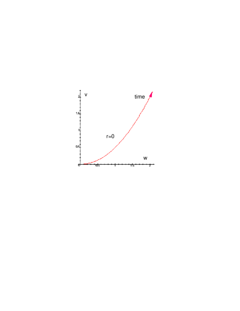
  Figure 1: An inertial world line, i.e., a section $r=0$ of Einstein – de Sitter space-time, embedded in $M_{5}$

  

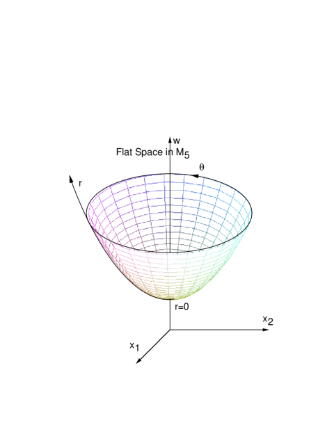
  Figure 2: Flat Euclidean space, embedded in the three-dimensional manifold of $M_{5}$ described by the coordinates $x^{1}$, $x^{1}$, $w$.

  

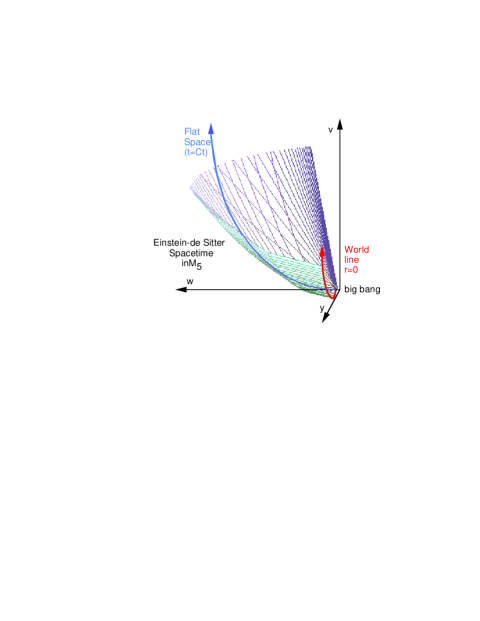
  Figure 3: The Einstein - de Sitter model (with flat spatial sections) embedded in a flat Lorentzian space. Both spatial sections ($t=Ct$) and inertial world lines ($r=Ct$) are parabolas.

Now I consider the general case (spatially flat, assuming $\lambda>0$), that I solve by defining $z:=\sqrt{\Omega_{m}/\lambda}\leavevmode\nobreak\ x^{3/2}$: the equation takes the form $dz^{2}=\alpha^{2}\leavevmode\nobreak\ (1+z^{2})\leavevmode\nobreak\ dt^{2}$, where $\alpha^{2}:=\frac{9\leavevmode\nobreak\ H_{0}^{2}\leavevmode\nobreak\ \lambda}{4}$, with the solution $z=\sinh(\alpha\leavevmode\nobreak\ t)$. Finally, the general solution is

$$x=(\Omega_{m}/\lambda)^{1/3}\leavevmode\nobreak\ [\sinh(\alpha\leavevmode\nobreak\ t)]^{2/3}.$$ (12)

All these models have a Big Bang, and I have chosen the integration constant so that $x=0$ at $t=0$. From this, we derive easily

$$\dot{x}=(\Omega_{m}/\lambda)^{1/3}\leavevmode\nobreak\ \frac{2\alpha}{3}\leavevmode\nobreak\ [\sinh(\alpha\leavevmode\nobreak\ t)]^{-1/3}\leavevmode\nobreak\ \cosh(\alpha\leavevmode\nobreak\ t),$$ (13)

and the Hubble parameter $H(t)=\frac{2\alpha}{3}\leavevmode\nobreak\ \coth(\alpha\leavevmode\nobreak\ t)$. The present period $t_{U}$ corresponds to $x=1$, or $H(t_{U})=H_{0}$, so that $\sinh\alpha\leavevmode\nobreak\ t_{U}=\sqrt{\lambda/(1-\lambda)}$.

The $r=0$ section of space-time is given by

$$x^{0}=[R(t)+S(t)]/2$$

$$x^{1}=0$$

$$x^{4}=[R(t)-S(t)]/2,$$

where $S(t):=\int^{t}\leavevmode\nobreak\ dt^{\prime}/\dot{R}(t^{\prime})$ has unfortunately no analytical expression.

I recall

$$v:=x^{0}+x^{4}=R(t)$$

$$x^{1}=R(t)\leavevmode\nobreak\ r$$

$$w:=x^{0}-x^{4}=S(t)+R(t)\leavevmode\nobreak\ r^{2}.$$

To be more specific, I illustrate (Fig. 4, 5) the case where $\Omega_{m}=\lambda/2=1/3$, which seems now favored by observational results. Then $\alpha^{2}:=\frac{3\leavevmode\nobreak\ H_{0}^{2}}{2}$, with the solution

$$x=(1/2)^{1/3}\leavevmode\nobreak\ [\sinh(\alpha\leavevmode\nobreak\ t)]^{2/3},$$ (14)

$$\dot{x}=(1/2)^{1/3}\leavevmode\nobreak\ \frac{2\alpha}{3}\leavevmode\nobreak\ [\sinh(\alpha\leavevmode\nobreak\ t)]^{-1/3}\leavevmode\nobreak\ \cosh(\alpha\leavevmode\nobreak\ t),$$ (15)

and the Hubble parameter

$$H(t)=\frac{2\alpha}{3}\leavevmode\nobreak\ \coth(\alpha\leavevmode\nobreak\ t).$$ (16)

The present period $t_{U}$ corresponds to $\sinh(\alpha\leavevmode\nobreak\ t_{U})=\sqrt{2}$.

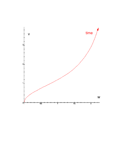
Figure 4: A world line of the $\lambda=2,\leavevmode\nobreak\ \Omega=2/3$ RW model, embedded in a flat Lorentzian two-dimensional space

Figure 5: RW model with $\lambda=2\omega=2/3$, embedded in a flat Lorentzian space

3.1.1 The matter dominated universes

As an other example, I consider the models where only non-relativistic matter governs the cosmic evolution, $\rho(x)=\Omega_{m}\leavevmode\nobreak\ x^{-3}$, so that

$$\frac{\dot{x}^{2}}{H_{0}^{2}}=\Omega_{m}\leavevmode\nobreak\ x^{-1}+1-\Omega_{m}.$$ (17)

More specifically, I illustrate (Fig.7) a spatially closed model, with $\Omega_{m}=2$. This model (hardly compatible with cosmic observations) has a Big Bang, a maximal expansion at $R=2/H_{0}$ and a Big Crunch. It appears advantageous to use $x^{0}$ as a parameter, with values 0, $R=4/H_{0}$ and $R=8/H_{0}$, respectively, for the three events. The parametric equations (4) take the form

$$x^{0}$$

$$x^{1}=\sin r\leavevmode\nobreak\ [2-2\leavevmode\nobreak\ (x^{0}/4-1)^{2}],$$

$$x^{4}=\cos r\leavevmode\nobreak\ [2-2\leavevmode\nobreak\ (x^{0}/4-1)^{2}].$$

In our representation, the space-time is represented by a revolution surface of an arc of parabola [Fig. (6)]. Spatial sections ($t=Ct$) are circles (3-spheres in ${\cal M}_{5}$). The world lines for inertial particles are the arcs of parabola between the Big Bang and the Big Crunch.

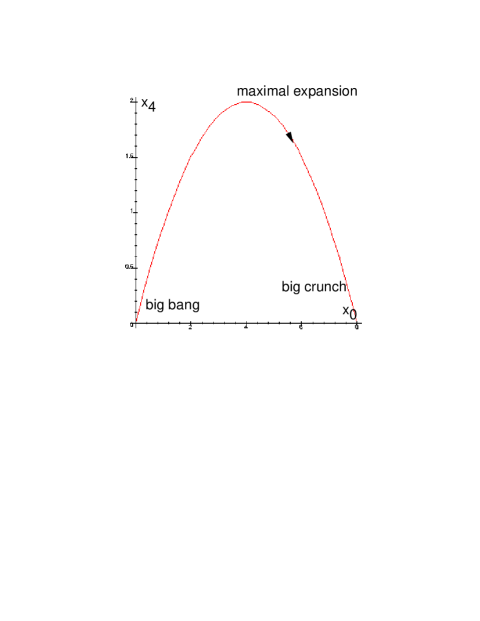
Figure 6: An inertial world line of a closed RW model, purely matter dominated, with $\Omega=2$, is an arc of a parabola.

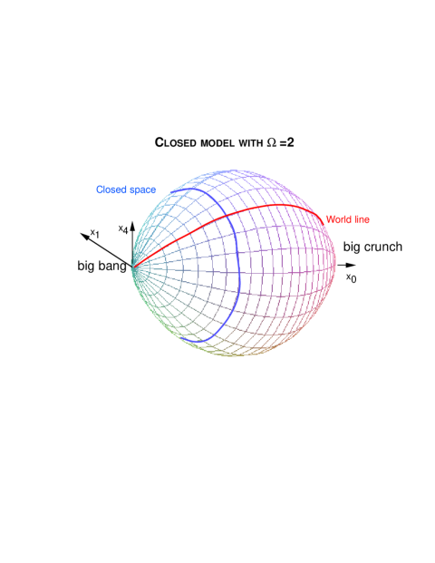
Figure 7: Closed RW model (purely matter dominated, with $\Omega=2$) embedded in a flat Lorentzian space. Spatial sections ($t=Ct$) are circles. Inertial world lines ($r=Ct$) are the arcs of a parabola illustrated in Fig(6).

4 Conclusion

These calculations generalize, to arbitrary Friedmann-Robertson-Walker models, the embedding usually used for the de Sitter models. The fact that the embedding space is flat offers a very good convenience to illustrate in an intuitive way the geometrical properties of these models. For instance, time durations, or lengths between events could be obtained by measuring (Lorentzian) lengths of the corresponding curves with a ruler in ${\cal M}_{5}$ or ${\cal M}_{3}$. Also, the curvature coefficients would be those obtained for the hypersurface in ${\cal M}_{5}$. Care must be taken, however, in this case, that the signature of the embedding space is Lorentzian. Many text books have illustrated this fact for the de Sitter case. Here we observe the curious fact that a flat space appears as a parabola (or a paraboloid in more dimensions). However, a correct measure of the curvature would confirm the flatness of the corresponding surface.

Beside their pedagogical interest, these representations could be of great help for various calculations. I mention for instance the calculation of cosmic distances or time intervals (generalizing those of Triay et al. (Triay (1996)) for the case of spatial distances). This would be also of great help to gain intuition in any theory with more than five dimensions.

Among other speculative ideas, it would be tempting to consider dynamics (here cosmic dynamics) as a geometrical effect in a manifold with 5 (or more) dimensions, which is flat (like here) or Ricci flat (this track is being explored by Wesson, Wesson (1994), and references therein).

This suggest prolongations of the present work in the spirit of the old Kaluza – Klein attempts: consider other solutions of general relativity (Wesson and Liu WessonLiu (2000)), consider solutions of gravitation theories other than general relativity, consider embeddings in Ricci-flat (rather than flat) manifolds, embeddings in manifolds with more dimensions, etc. For instance, Darabi et al. (Darabi (2000), see also references therein) suggest that this may offer a starting point for quantum cosmology. This may also offer an angle of attack for quantization in curved space time, following the work already done in de Sitter space-time. This is motivated by recent work (see, e.g., Bertola et al. 2000 and references therein) which have shown interesting relations between quantum field theories in different dimensions (for instance, they suggest the idea that ‘ a thermal effect on a curved manifold can be looked at as an Unruh effect in a higher dimensional flat spacetime ‘).

References

• (1) Bertola M., Gorini V., Moschella U., Schaeffer R. 2000, hep-th/ 9906035 v2
• (2) Darabi F., Sajko W. N. and Wesson P. S. 2000, gr-qc/ 0005036
• (3) Hawking S. W. and Ellis G. F. R., The large scale structure of space-time, Cambridge University Press1973
• (4) Kaluza Th. Sitz. Preus. Akad., 966, 1921
• 1926, (1927) Klein O., Zeits. F r Phys., 37, 895, 1926 ; Nature, 118, 516, 1927
• (6) Souriau J. - M., Nuovo cimento, XXX, 2, 1963
• (7) Thiry Y., Journal Math. Pures et Apppl., 9, 1 (1947)
• (8) Triay R., Spinelli L. and Lafaye R. 1996, MNRAS 279, 564-570
• (9) Wesson, P. S. 1994, Ap.J., 436, 547-550
• (10) Wesson P. S. and Liu H. 2000, gr- qc/ 0003012