Spiral and irregular galaxies in the Hubble Deep Field North

Abstract

We analyze a morphologically-selected complete sample of 52 late-type (spiral and irregular) galaxies in the Hubble Deep Field North with total K-magnitudes brighter than K=20.47 and typical redshifts $z\sim 0.5$ to 1.4. This sample exploits in particular the ultimate imaging quality achieved by HST in this field, allowing us to clearly disentangle the early- from late-type galaxy morphologies, based on accurate profiles of the surface brightness distributions. Our purpose was to investigate systematic differences between the two classes, as for colours, redshift distributions and ages of the dominant stellar populations. Our analysis makes also use of an exhaustive set of modellistic spectra accounting for a variety of physical and geometrical situations for the stellar populations, the dusty Interstellar Medium (ISM), and relative assemblies. The high photometric quality and wide spectral coverage allow to estimate accurate photometric redshifts for 16 objects lacking a spectroscopic measurement, and allow a careful evaluation of all systematics of the selection [e.g. that due to the surface-brightness limit]. This sample appears to miss significantly galaxies above $z=1.4$ (in a similar way as an early-type galaxy sample previously studied by us), a fact which may be explained as a global decline of the underlying mass function for galaxies at these high redshifts. Differences between early- and late-types are apparent – particularly in the colour distributions and the evolutionary star-formation (SF) rates per unit volume –, although the complication in spectro-photometric modelling introduced by dust-extinction in the gas-rich systems prevents us to reach conclusive results on the single sources (only future long-wavelength IR observations will allow to break the age/extinction degeneracy). However, we find that an integrated quantity like the comoving star-formation rate density as a function of redshift $\Psi(z)$ is much less affected by these uncertainties: by combining this with the previously studied early-type galaxy sample, we find a shallower dependence of $\Psi(z)$ on $z$ between $z=0.2$ and $z=1.5$ than found by Lilly et al. (lilly (1995)). Our present results, based on a careful modelling of the UV-optical-NIR SED of a complete galaxy sample – exploiting the observed time-dependent baryonic mass function in stars as a constraint and attempting a first-order correction for dust extinction – support a revision of the Lilly-Madau plot at low-redshifts for both UV- and K-band selected samples, as suggested by independent authors (Cowie et al. cowie (1999)).

1 INTRODUCTION

Cosmogonic models, in particular those based on the hierarchical clustering of cold dark matter halos, now including detailed physical descriptions of gas cooling, star-formation and feed-back processes in the baryonic component, make specific predictions about the evolutionary history of galaxy populations as a function of their morphology.

Basically, in the hierarchical scheme, forming galaxies acquire angular momentum from tidal interactions with the surrounding structure and then dissipate and collapse preferentially along the rotation vector and tend to form flattened rotational-supported structures (disk galaxies). There are indeed indications of a substantial population of large structures of this kind up to the highest redshifts from absorption-line studies in the distant quasar spectra (e.g. Wolfe A.M. wolfe (1999)). The pressure-supported stellar bulges dominating E/S0 galaxies, in this scheme, would originate from the violent relaxation and dynamical evolution following strong interactions and mergers of primordial disk galaxies. At the zero-th order, these models predict that spheroidal galaxies are assembled somewhat later than spirals, although their stellar populations might not differ much if the merger occurs among gas-poor systems. One such extreme case has been discussed by Kauffmann & Charlot (kauffmannb (1998)) based on the $\Omega=1$ standard CDM cosmology, predicting a substantial dearth of spheroidal galaxies already by z=1, most of them being formed at lower z.

More recently it has been pointed out that, within this scheme, the morphological appearence of a galaxy may repeatedly change with cosmic time not only from a late- to an early-type following a merging event, but also from a spheroidal to a disk configuration following the acquisition of new infalling gas from the environment (e.g. Ellis R.S. ellis (1997)). This may reflect in long-wavelength (V to K) colour distributions un-distinguishable between early- and late-types, while shorter-wavelength (U to V) colours would be dominated by the on-going SF in disks.

An opposite pattern is contemplated by the ”traditional” models of galaxy formation, assuming that massive galaxies, in particular elliptical and S0’s, originated first at high redshifts as single entities from rapid homologous collapse of primordial gas. Gas-rich systems, in this view, form instead more quiescently from progressive inflow of gas into the dark matter halos during most of the Hubble time. This formation scenario then predicts a marked differentiation in colours and ages for the stellar populations of the two classes of galaxies, late-type galaxies containing much younger stellar populations on average than the early-types. Also a substantial population of massive spheroids would be expected to be visible at $z\sim 2$ in this case.

The ultra-deep integrations at various wavelengths performed by the Hubble Space Telescope in the Hubble Deep Field (Williams et al. williams (1996); we consider here only the survey in the North area) offer an extremely valuable dataset to study morphological properties of high-redshift galaxies. Furthermore, the very accurate photometry achievable in such deep images allows accurate estimates of the photometric redshifts for vast numbers of faint galaxies in the field.

We have recently exploited these data to study the colours, masses, age distributions, and the star-formation history of a sample of elliptical-S0 galaxies (Franceschini et al. franceschini (1998), FA98 hereafter). The basic result was to find colours indicative of wide ranges of ages for the stellar populations and a remarkable absence of objects at $z>1.3$, both facts telling against the predictions of the ”traditional” monolithic formation scenario.

As a natural complement, we present in this paper an analysis of late-type and irregular galaxies in the HDF. Similarly to what we did there, our primary selection is in the K-band, obtained from a deep KPNO image, to minimize the biases in the sample due to the effects of K- and evolutionary corrections. The completion of our previous analysis of E/S0 to account for the complementary set of late-type systems is also needed for a global evaluation of the star-formation history as a function of redshift. The advantage of our approach over previous attempts (Lilly et al. lillyb (1996), Cowie et al. cowie (1999)) is in our careful treatment of dust extinction from a detailed fitting of the UV-optical-NIR spectral energy distributions (SED). In addition, the detailed knlowledge of the near-IR (NIR) spectrum for sources at the relevant redshifts is informative on the baryonic mass function in stars, which provides an essential constraint on the cumulative star-formation rate as a function of time.

In Section 2 we discuss the selection scheme and photometric corrections used to construct a complete K-band flux limited sample of late–type galaxies. In Section 3 we describe the population synthesis code that we used to model the optical-NIR SEDs of our sample objects, taking into full account the effects of a dusty interstellar medium in the galaxy spectra. Our main results are then reported in Section 4, where we perform detailed analyses of the space distributions, colours and ages of the stellar populations of field spiral and irregular galaxies, compared with ellipticals and S0. We discuss the difficulties inherent in the spectral modelling of gas-rich systems affected by dust extinction. We finally attempt to construct the global star formation histories of field galaxies (E/S0+spiral/irregulars). In Section 5 we summarize our main conclusions.

We anticipate that the results of the present analysis, based on a survey over a very small sky field, are to be considered as only tentative, untill larger areas will be surveyed to similarly deep limits.

We adopt $H_{0}=50\leavevmode\nobreak\ Km\leavevmode\nobreak\ s^{-1}\leavevmode\nobreak\ Mpc^{-1}$ throughout the paper. For consistency with FA98 the analysis is made assuming $q_{0}=0.5$, and zero cosmological constant $\Lambda$.

2 SAMPLE SELECTION AND PHOTOMETRY

The Hubble Deep Field North has been observed in 4 broad bands (F300W, F450W, F606W, F814W) for a total of 150 HST orbits by Williams et al. (1996), and constitutes the deepest ever exposure on a small sky area. Accurate photometric data in the four bands have been published for thousands of faint galaxies by the authors.

Dickinson et al. (dickinson (1997)) observed the HDF–North in the near-IR with the IRIM camera on the KPNO 4 m telescope. The camera employs a 256 $\times$ 256 NICMOS-3 array with 0”.16 pixel^-1, but the released images were geometrically transformed and rebinned into a 1024 $\times$ 1024 format. IRIM exposures have been secured in the $J$, $H$ and $K$ filters, for a total of 12, 11.5 and 23 hours, respectively. Formal 5 $\sigma$ limiting magnitudes for the HDF/IRIM images, computed from the measured sky noise within a 2” diameter circular aperture, are 23.45 mag at $J$, 22.29 mag at $H$, and 21.92 mag at $K$, whereas the image quality is $\sim$ 1”.0 FWHM.

Our sample of galaxies has been extracted from the HDF/IRIM $K$-band image through a preliminary selection based on the automatic photometry provided by SExtractor (Bertin $\&$ Arnouts bertin (1996)). It is flux limited in the $K$ band and it excludes early–type galaxies, i.e. objects whose surface brightness distribution is dominated by a de Vaucouleurs profile.

To determine the limit of completeness in the $K$ band (hereafter $K_{L}$) for inclusion in our sample, we followed the same empirical procedure described in FA98. Briefly, a large number of toy galaxies with exponential profiles (produced with the IRAF-MKOBJECTS tool) have been used to check the performances of Sextractor in estimating the K-band magnitudes ($K_{SEx}$) of late-type galaxies. This allowed us to determine the magnitude $K_{lim}$ below which the scatter $\sigma_{K_{SEx}}$ of the measured magnitudes turns out to be lower than some given value $\sigma_{max}$ (the vertical line in Figure 1a corresponds to $K_{lim}=21$ and $\sigma_{max}=0.18$). Moreover, using only galaxies with $<K_{SEx}>\leq K_{lim}$, we have derived the following empirical relation between the bias $\Delta K=<K_{SEx}>-K_{true}$ and the effective surface brightness $<\mu_{e}^{K}(SEx)>$ (see Figure 1b):

$$\log\Delta K=-1.059+0.188<\mu_{*}^{K}>+0.061<\mu_{*}^{K}>^{2}$$

$$+0.006<\mu_{*}^{K}>^{3},$$ (1)

where $<\mu_{*}^{K}>=<\mu_{e}^{K}(SEx)>-21$. This relation provides the true total $K$ magnitudes from the SExtractor measured flux. Then simulations have shown that the K-band image has a surface brightness limit of $<\mu_{e}^{K}(SEx)>=23.$

Figure 1: Left panel: standard deviation of the SExtractor magnitude estimates as a function of the average magnitude for galaxies in the simulated images: the standard deviation is very small for $<K_{SEx}>\leq 21^{m}.0$. Right panel: difference between true flux and the SExtractor flux as a function of the average surface brightness for the subsample of simulated galaxies with $<K_{SEx}>\leq 21^{m}.0$.

By analogy with FA98, we have first produced a catalog of morphologically selected late-type objects with $K_{SEx}\leq K_{lim}=21.0$; then we have used effective radius estimates from high resolution (HST) optical imaging to derive the effective surface brightness of galaxies ($<\mu_{e}^{K}>$); finally, we have applied to the $K_{SEx}$ magnitudes the statistical corrections given by equation [1] and we have included in the final sample only galaxies with corrected magnitudes less than or equal to $K_{L}=K_{lim}-\Delta K_{max}-\sigma_{max}=20.47$ mag (we assume $\Delta K_{max}\sim 0.35$ from Figure 1b).

Figure 2: Observed broadband spectra for sixteen galaxies in our sample, fitted with the synthetic models described in Section 3.

A total of 176 objects with $K_{SEx}\leq 21$ mag were detected by SExtractor in the IRIM $K$-band image. After carefull inspection of the high resolution HST images, we rejected all elliptical and S0 galaxies (including the 35 early-type objects identified in FA98) and the stars. A few objects were also rejected from the sample due to their position in the frame (at the edges of the image the noise is higher and the magnitude estimate is likely to be uncertain). We then produced a first preliminary, incomplete sample of late–type galaxies.

The effective radii $r_{e}$ were estimated running SExtractor on the WFPC2 $V_{606}$ frame with the parameter $FLUX\_RADIUS$, providing the radius containing half of the total emitted flux. The surface brightness $<\mu_{e}^{K}(SEx)>$ was evaluated for each galaxy and the statistical corrections $\Delta K$ were computed using the eq (1).

The final complete sample of late-type galaxies with $K_{corr}<20.47$ consists of 52 objects over the HDF area of 5.7 square arcmin. For 36 objects we have the spectroscopic redshift (Cohen et al. cohen (1996), Cowie et al. cowie (1999), Fernandez-Soto et al. soto (1998)), while for the remaining 16 we measured it from our photometric analysis as described below.

A procedure analogous to that outlined for the K band was used to derive, for each object of the selected sample, the corrected magnitudes in the J and H bands.

The optical magnitudes in the F300W, F450W, F606W and F814W bands (U, B, V and I in Table 1, respectively) have been computed again with SExtractor on the high resolution WFPC2 images (no corrections being applied in this case). Magnitudes are in the AB system, defined by the relation (Oke $\&$ Gunn oke (1983)):

$$AB=-2.5\log F_{\nu}-48.60$$ (2)

where $F_{\nu}$ is the flux in $erg\leavevmode\nobreak\ cm^{-2}\leavevmode\nobreak\ Hz^{-1}$, the constant beeing choosen so that $AB=V$ for an object with flat spectrum.

Some data on the sample are listed in Table 1. Column 1: our identification; column 2-4: coordinates $\alpha$ and $\delta$ (at J2000). To these must be added 12 hours 36 minutes (RA) and 62 degrees (Dec); column 5: $r_{e}$ is the effective radius, in arcsec, derived from HST images; column 6-9: optical U, B, V, I magnitudes in the AB system (see above); column 10-12: near-infrared J, H, K corrected magnitudes in the standard system; column 13: redshift of each object. Values in brackets are photometric redshifts, while the other are all spectroscopic.

3 MODELLING GALAXY SEDs IN THE PRESENCE OF A DUSTY ISM

The optical-NIR SEDs of our sample objects have been modelled using the population synthesis code GRASIL (Silva et al. silva (1998)), taking into full account the effects (optical extinction and thermal reprocessing) of a dusty interstellar medium in galaxy spectra. We defer the reader to that paper for a through description of this model and for precise definitions of the parameter, while for convenience we summarize the main features below.

3.1 The GRASIL code

The code provides a self-consistent description of the formation and evolution of a galactic system in its various stellar and ISM components, including its secular evolution during the Hubble time and episods of enhanced star-formation possibly following interactions and mergers.

As a preliminary step the code allows to solve the equations ruling the chemical evolution, providing the star formation and metallicity histories SFR(t) and Z(t) as a function of time. The computations presented here were performed adopting one–zone (no spatial dependence) open models including the infall of primordial gas, according to the standard equations of galactic chemical evolution. As usual, the star formation rate is determined by the amount of gas in the system according to a Schmidt-type law

$$SFR(t)=\nu\,M_{g}(t)^{k}.$$

We have generated 3 different $SFR(t)$, in order to provide a wide range of spectral evolution patterns. The peak occurs at about 1, 2 and 3 Gyr (hereafter model (a), (b) and (c) respectively), getting broader from (a) to (c). As a result, half of the final stellar mass $M$ (i.e. at 13 Gyr) has been assembled at galactic times of 2, 3.7 and 4.7 Gyr in the three cases respectively. A standard Salpeter IMF between 0.1 and 100 $M_{\odot}$ is assumed.

As described by Silva et al. (1998), GRASIL calculates self-consistently the absorption of starlight by dust, the heating and thermal emission of dust grains, for an assumed geometrical distribution of the stars and dust, and a specific grain model.

In the GRASIL model several parameters affect the overall modifications imprinted by dust on the SED. However, if we confine ourselves to the attenuation of stellar radiation in the optical/UV/NIR bands, we can obtain most of the possible spectral behaviours by adjusting only two quantities: the $escape\leavevmode\nobreak\ timescale\leavevmode\nobreak\ t_{o}$ (see Eq [8] in Silva et al. 1998 for a precise definition) of newly formed stars from parent molecular clouds (MCs) and the total mass of dust. Indeed $t_{o}$ controls the fraction of light from very young stellar generations hidden inside MCs and converted to IR photons, since the MCs optical thickness is very high below $\sim 1\mu$m (cfr. Silva et al. 1998). On the other hand, the effects of the diffuse (cirrus) dust depend on several quantities: the radial and vertical scale lengths for stars and dust distributions $R_{d}$ and $z_{d}$, the residual gas in the galaxy $M_{g}$, the dust to gas ratio $\delta$ and the fraction of gas which is in the MCs component $f_{mc}$. However we found that most, if not all, the possible attenuation laws of the diffuse dust, arising from different choices of these quantities, can be closely mimicked by simply adjusting the amount of gas, while fixing the other quantities to the ‘typical’ values: $R_{d}=3.5(M/10^{11}M_{\odot})^{1/3}$ Kpc, $z_{d}=0.1\,R_{d}$, $\delta=0.01$ and $f_{mc}=0.5$. Obviously, while different choices of $M_{g}$, $R_{d}$, $z_{d}$, $\delta$ and $f_{mc}$ can yield similar attenuation laws on the optical spectrum, the spectral shapes of the corresponding IR continuum re-radiation can be rather different.

Figure 3: Comparison of photometric redshifts, based on seven-band spectral data, with spectroscopic redshifts. Error bars refer to interval solutions with more than 90$\%$ confidence level, derived from $\chi^{2}$ fitting using models [a] and [c].

Strictly speaking the residual gas $M_{g}$ is not a parameter, being instead the outcome of the chemical evolution code, through the Schmidt law. However we use the trick of forcing $M_{g}$ to different values, in order to describe with a monoparametric sequence the effects of a global attenuation on the SED. Besides this, a larger ‘freedom’ on $M_{g}$ takes into account that the Schmidt law should not be taken too literally, as a strict relationship between the total gas content and the $SFR$ in the system. The law may only provide an order of magnitude description, in particular for the secular evolution of the SFR, the so-called ”inactive phase” of galaxy evolution bringing essentially to the formation of spiral disks. Several other physical parameters influence the rate of star-formation with respect to the simple available amount of residual gas, in particular the gas pressure and temperature, which may drastically change as a consequence of a violent dynamical event, like an interaction or a merger, followed by gas compression and efficient cooling. Overall, we use the criterion of considering acceptable values from 0.2 to 5 times the ‘true’ $M_{g}$ given by the chemical evolution code.

3.2 An extensive grid of model template spectra

The code allowed us to build a very large set of model spectra describing all possible age and mass distributions for the stellar populations, for the dusty ISM, and relative assemblies.

For each of the 3 histories SFR(t) we have generated two grids of models: one with $t_{o}=5$ Myr and another with $t_{o}=30$ Myr. Silva et al. (1998) found that the former value is typical for normal spirals while the latter is more suited for starbursting systems. Each of these grids consists of 1400 models computed with ages $t_{G}$ ranging from 0.2 to 10 Gyr in steps of 0.2 Gyr and $M_{g}$ from 0 to 1 (in units of the final mass of stars) in 28 logarithmic steps.

In total we have therefore $1400\times 2\times 3=8400$ model spectra with different age, gas content, MCs escape timescale, and $SFR(t)$ which we compared with the observed sample SED, allowing for the obvious scaling in luminosity.

In addition we considered one further grid of spectra to see how our observed SEDs compare with those expected for spheroidal systems: for these we used the $SFR(t)$ (c) model, but truncated at 3 Gyr to simulate the onset of a galactic wind. The adopted geometry in this case was a modified King profile (Eq. [3] in Silva et al. 1998) with $r_{c}=0.15(M/10^{11}M_{\odot})^{1/3}$ Kpc.

An example of the resulting fits to the observed broadband spectra of sixsteen galaxies in our sample is reported in Figure 2. The analysis of the 52 fitted SEDs reveals the presence of two dominant different kinds of spectral behaviours: (a) objects which are red and show a strong convergence in the UV region, and (b) blue spectra that are flatter at all wavelengths, dominated by young stellar populations.

Figure 4: Scaling of the observed average surface brightness for two faint galaxies in our sample as a function of redshift, according to the evolution models (a) for galaxy # 16 and (c) for # 50 respectively. Note that galaxy # 50 is the one with the lowest observed value of the surface brightness. The deep K-band image used in the primary selection has a $3\sigma$ limiting brightness of $23\ K\ magnitudes/arcsec^{2}$.

Figure 5: Redshift distribution for spiral and irregular galaxies brighter than $K=20.47$ in the HDFN. The continuous line is the predicted distribution based on canonical local luminosity functions for late-type and irregular galaxies and the spectral evolution model (c) mentioned in Sect. 3.1.

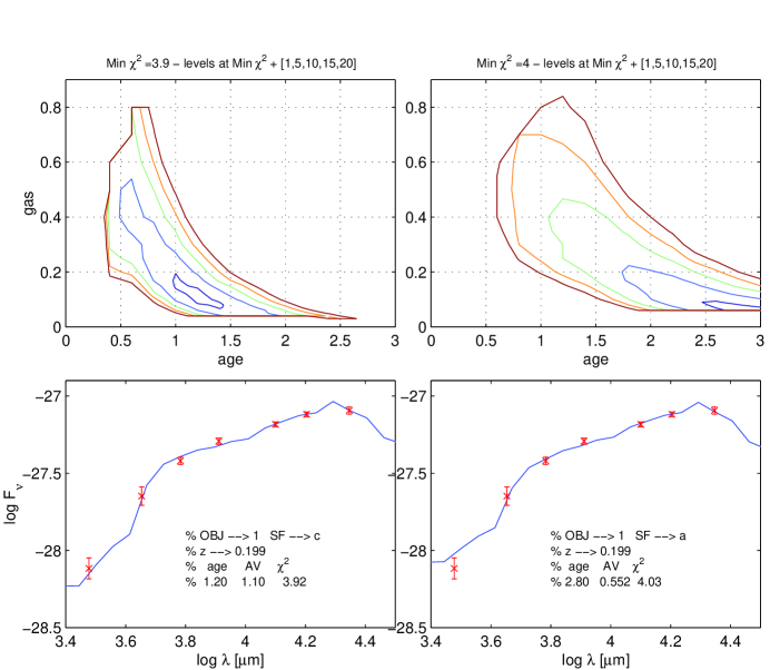
Figure 6: Examples of different fits to the observed broad-band spectra of object number 1, fitted with the population synthesis models described in Sect. 3. The figure plots $\chi^{2}$ contours for the amount of dust-rich gas versus the age (top panels) and the corresponding best-fit spectra for two different histories of SF (lower panels). The solution on the right refers to the model [a] in Fig. 2 and a value for the escape timescale $t_{o}$ of 5 Myr (see Sect. 3.1 for details about these parameters). On the left: solution for model [c] and $t_{o}=30$ Myr. The contours correspond to a $\chi^{2}$ increment of 1,5,10,15 and 20 with respect to the best fit in the grid. Therefore the second innermost contour correspond to the 90% confidence interval.

Figure 7: For three representative objects in our sample ($\#$ 1, 30 and 36) located at different redshift (z = 0.199, 1.355 and 0.559 respectively) we plot various solutions for the rate of on-going SF against the average V-band effective extinction $A_{V}$. We report the best-fit solutions for every different history of SF considered (as described in Sect. 3.2) and two more corresponding models: the youngest and the oldest one with $\chi^{2}=\chi^{2}_{best}+5$. The labels near the points are the $\chi^{2}$ values for each solution. This figure illustrates the fact that the observed SEDs can be fitted with models differing in the current rate of star formation by factors up to 5-10.

4 RESULTS

4.1 The space-time distribution of K-band selected late-type galaxies

The grid of model spectra has been used to estimate redshifts from spectral fits to the 7-band photometric data for the 16 galaxies lacking a spectroscopic measurement. As typical in cases in which such a wide spectral coverage (0.3 to 2.2 $\mu m$) and accurate photometry are available, the relative errors in $z$ turn out to be quite small, of the order of $\sim 10\%$. These broad-band spectral fits allow quite robust estimates of redshifts also for dusty objects, mostly exploiting a well-characterized feature of the optical spectra, the Balmer discontinuity, which is weakly affected by dust extinction (cfr discussion in section 3.2.1 in FA98).

Figure 8: Example of two different fits to the observed broad-band spectrum for object number 30 in our identification. We report the spectral galaxy emission of two dusty environments (Sect. 3.1): dashed line = diffuse ISM (cirrus), dot-dashed line = molecular clouds (MCs). The solid line corresponds to the total integrated spectrum of the galaxy. Solution 1 (top panel) and 2 (bottom panel) refer to that plotted in Fig. 7 for object 30, corresponding to a value of $A_{V}\sim 1.9$, with SFR $\sim 180M_{\odot}/yr$, $\chi^{2}=6.77$ (for sol1), and SFR $\sim 420M_{\odot}/yr$, $\chi^{2}=7.44$ (for sol2).

To check the consistency of our method, we compare in Figure 3 our photometric redshift predictions with the corresponding spectroscopic measures. The vertical error bars refer to different solutions at better than 90$\%$ confidence, derived from a $\chi^{2}$ fitting procedure using models (a) and (c). Fig.  3 shows overall good agreement within our modellistic uncertainties of the fits. Added to the 36 spectroscopic redshifts, this procedure enabled us to get quite a reliable redshift distribution for our sample objects.

The distribution in redshift of a source population from a complete flux-limited catalogue provides a powerful constraint on its evolutionary history and formation epoch. This obviously assumes that we control with reasonable confidence all possible selection effects, in particular those due to the surface brightness limit, the cosmological dimming and K-corrections to the fluxes. If some morphological criteria are at play, one needs also to understand how morphological appearence may evolve with redshift. In our case the control of the selection effects is made easier by our primary selection in the K-band, which implies minimal K- and evolutionary corrections as a function of redshift.

The availability of accurate measurements of the effective radii $r_{e}$ allows to control the effects of the limiting surface brightness observable in the field in K, which we evaluated from the simulations described in Sect. 2 to be $<\mu_{K}>\simeq 23\ magnitudes/arcsec^{2}$.

Figure 4 shows the evolution of the observed surface brightness for two objects in our sample (including the galaxy with the faintest surface brightness) as a function of redshift, taking into account the cosmic dimming and using a variety of spectral evolution patterns corresponding to the models described in Sect. 3. It is clear from the figure that the cutoff in surface brightness in the IRIM K band image has no impact in our selection process above our adopted limit in total magnitude of $K<20.47$, and the whole redshift space up to at least $z=2.5$ is clearly accessible in principle.

Figure 5 reports the histogram of the observed redshifts for our complete $K<20.47$ sample (including the 16 photometric estimates). The distribution shows pronounced peaks at $z\sim 0.5$ and $z\sim 1$, clearly indicative of strong inhomogeneities in the source distribution due to spatial clustering in the relatively small volume sampled by the HDFN. The uncertainty due to clustering in the limited volume has to be kept in mind when drawing any conclusions from our analysis, which require confirmation from surveys on more extended areas.

A second relevant feature is apparent in Fig. 5: a cutoff at $z\sim 1.4$, with only 2 objects out of 52 found above this limit.

We compared this distribution with a model prediction based on the local luminosity function of galaxies in the K-band (Gardner et al. gardner (1997)) complemented with information on the contributions of various morphological classes from optical data (see Franceschini et al. 1998 for more details). The luminosity function is then evolved according to spectral model (c), which provides a conservative estimate of the number of $z>1$ galaxies (it has the minimal evolution rates among the three models considered). The other assumption we made is that the luminosity function changes as an effect of the evolution of the $M/L$ ratio ($M$ changes because more mass is turned into stars with time, $L$ follows the evolution of the stellar populations). The onset of star-formation is assumed to happen at $z=4$.

As shown in the figure, these assumptions would imply an expected number of late-type galaxies at $z>1.5$ significantly in excess of the observations (9 expected versus only 1 observed). This result parallels a similar finding by FA98 and Rodighiero, Franceschini and Fasano (2000) for the early-type population, showing a demise of objects at redshifts larger than $z\sim 1.3$. One of the possible interpretations of this effect given by FA98, i.e. that the morphological selection could miss galaxies with shapes deviating from the De Vaucouleurs profile in case of merging activity at these redshifts, is no longer acceptable: essentially there are no bright ($K<20.5$) galaxies altogether at $z>1.4$ in the HDFN area.

4.2 Evaluating galactic ages and extinction properties

As anticipated, if the photometric measurement of redshift from broad-band spectral fits is weakly affected by dust extinction, the estimates of most other physical parameters of gas-rich systems suffer quite more by the uncertain amount of dust and from the degeneracy between ages of stellar populations and extinction. To check this we have used our large grid of model spectra to study the degeneracy of the spectral-fitting solutions of our sample galaxies.

Figures 6 plots $\chi^{2}$ contours for the amount of dust-rich gas versus the age for two representative galaxies, as well as the best-fit spectra for two different histories of SF (model [a] and [c]).

It is immediately apparent that, even within sets of models based on the same evolutionary SFR(t), a fairly substantial degeneracy exists between the age and amount of dust. Furthermore, rather different star formation histories can lead to equally good fits, as detailed in Fig. 6.

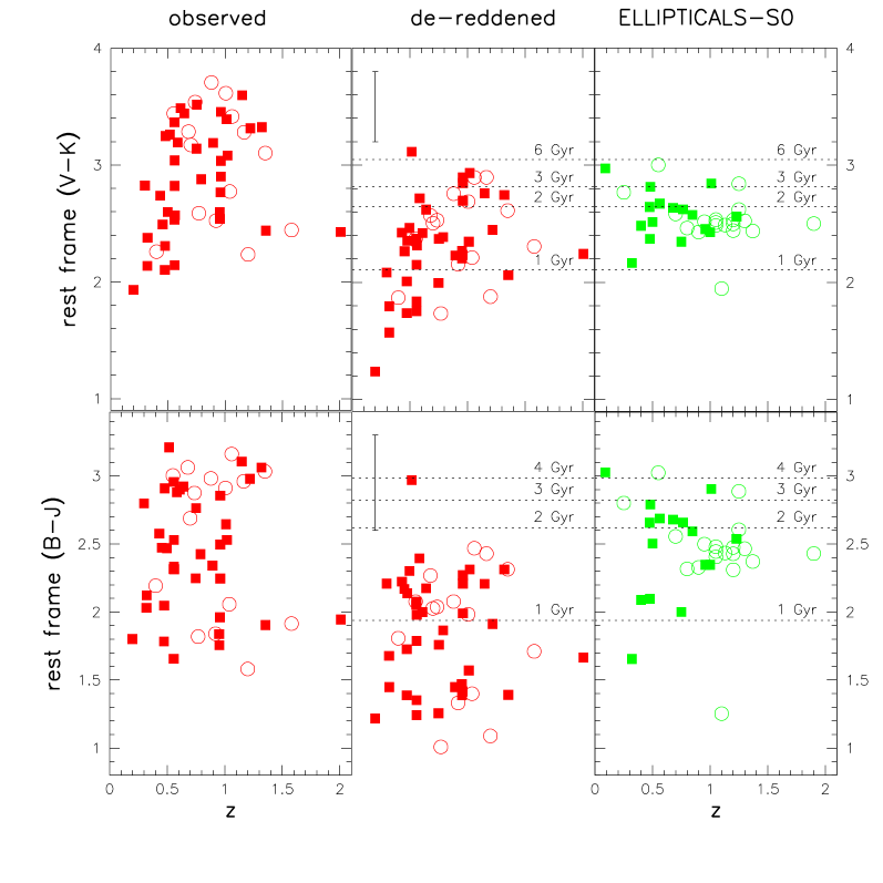
Figure 9: Rest frame (V-K) (upper panels) and (B-J) (lower panels) colours of late–type field galaxies, compared with predicted values for single stellar populations with solar metallicity. The ages for the latter are indicated as well the mean colours of local galaxies. The left two panels refer to the observed colours, on the center we present the corresponding ”de-reddened” colours based on our best-fit SED solutions. On the right we report the rest-frame colours of ellipticals and S0 galaxies from FA98. Filled squares refer to objects with spectroscopic redshift, open circles to those with photometric redshift. The error bars shown in the central panels correspond to the uncertainty in the dereddening at 90% confidence.

Figure 7 summarizes some results of our best-fitting procedures for three representative objects in our sample. For each object, it reports various solutions for the rate of on-going SF and the average V-band extinction $A_{V}$, including the corresponding values of the $\chi^{2}$. This figure illustrates the fact that the observed SEDs can be fitted with models differing in the current rate of star-formation by factors up to 5–10: a large amount of SF activity can be easily hidden at wavelengths below a few $\mu$m.

Figure 8 details the results of two different fits to the observed broadband spectrum for object 30, clearly illustrating the degeneracy existing between SF and extinction. The two SEDs correspond to two solutions reported in Fig. 7, with values of the SFR differing by a factor $\sim 2.5$. The top panel refers to the solution 1 with $\chi^{2}=6.77$ and SFR$\sim 200M_{\odot}/yr$. The lower panel refers to solution 2 with $\chi^{2}=7.44$, SFR$\sim 400M_{\odot}/yr$. It is clear that if the analysis is confined to optical/NIR wavelenghts, it cannot clearly discriminate between the two solutions, whose differences are apparent only including the far infrared spectrum, where dust re-emission would be detectable. Only observations of the IR spectral energy distribution, say between a few tenths up to a few hundreds $\mu$m, where actively star forming galaxies emit most of the energy, would allow to break the present degeneracy in the solutions.

4.3 Colours, sizes and average surface brightness of late-type galaxies at high redshifts

As a first assessment of the age and extinction distributions, we report in Figure 9 the rest frame (V-K) and (B-J) colours as a function of redshift. As in FA98, the rest frame (B-J) colours are computed by interpolating the observed galaxy spectra using the best-fit models listed in Table 1 (see Sect. 4.4), while the (V-K) colours require a slight extrapolation to longer wavelenghts. The left two panels refer to the observed spectra, which include the effects of reddening, while the colour distributions reported in the central panels correspond to ”de-reddened” spectra (i.e. taking out the effect of extinction and showing the underlying colour distribution). As we see, extinction plays a significant role: the estimated absorption-subtracted colours appear on average bluer by one magnitude. De-reddened colours are compared with the predictions of single stellar populations with solar metal abundances (dashed horizontal lines). The vertical error bars in the central panels are the mean uncertainties related to our de-reddening procedure based on our grid of models and our adopted 90% confidence level.

A comparison with the early–type galaxy sample studied by FA98 indicates that our late–type field galaxies present redder colours on average, because of extinction. This evidence is stronger in the (V-K) distribution, where a remarkable excess of red late–types is apparent at $z>0.5$ and $V-K>3$. This illustrates that selecting by colours is far more sensitive to extinction effects than to intrinsic differences among the stellar populations contributing to the flux.

Once de-reddened, the rest-frame (B-J) colours reveal young stellar populations with ages from 0 to 2 Gyrs, significantly bluer than those of early-type galaxies, indicative of on-going SF. The (V-K) de-reddened colours show a dependence on redshift: while at $z<0.6$ they appear blue, those for galaxies at $z>0.7$ are constant and quite red on average ($2<V-K<3$), and as red as those of the early-type population investigated by FA98.

We warn that translation to age-distributions is subject to the uncertainties in the evaluation of the effective extinction (see also next Section). However, the similarity in the intrinsic V-K colours of galaxies independent of morphology does indeed support a common age distribution for the spheroidal stellar components in Elliptical/S0s and in spiral bulges, something predicted by the hierarchical formation scenario mentioned in Section 1.

Finally, we report in Figure 10 our measured average surface brightness in the B band ($<\mu_{B}>$) versus effective radius $R_{e}$ for the bona-fide spirals in our high-z sample, compared with data from a local sample based on the RC3. $<\mu_{B}>$ was computed for our distant sources applying only the K-correction and the cosmological scaling factors. A further correction has been applied taking into account the effects of internal absorption. While the largest values of $R_{e}$ shown by local galaxies are missed by our high-z sample because we are not sampling the rare population of large size galaxies in the HDF limited space volume, there is no evidence of a significant offset in $<\mu_{B}>$ between the local and distant spirals within the large observed spreads in the data. In particular, the lowest surface brightness galaxies ($<\mu_{B}>\simeq 22-23$) in our sample are highly inclined, probably extinguished, objects. Note that the same relation fitting the Kormendy relation for E/S0 galaxies also fits data for spirals.

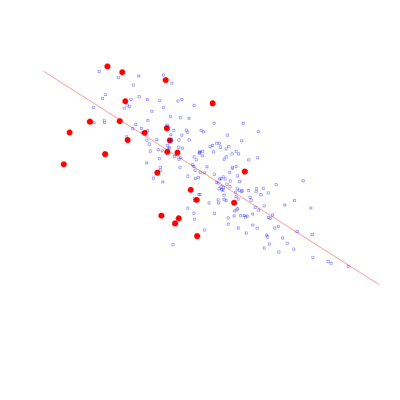
Figure 10: Kormendy relation in the B band, i.e., the average surface brightness versus effective radius for the bona-fide spirals in our high-z sample (filled cirles), compared with the data from a local spiral sample based on the RC3 (open squares). $<\mu_{B}>$ was obtained for our distant sources applying the K-correction and a correction for the internal absorption.

4.4 A tentative physical characterization of late-type galaxies in the HDF-N

Though aware of the uncertainties inherent in the spectral modelling of gas-rich systems due to the uncertain extinction, neverthless we attempt here to estimate some basic physical parameters of these sources, or at least to provide some boundary values as found by application of our vast model grid.

We report in Table 1 the formal best-fit solutions obtained from fitting the observed SEDs of our sample galaxies: $A_{V}$: V band effective extinction; $M_{tot}$: total baryonic mass divided by $10^{11}$ solar masses; $SFR$: observed SFR in solar masses per year.

Figure 11: Panel $a$: Distribution of the on-going star formation rate SFR versus redshift, for the best-fit solutions. Panel $b$: SFR against the total baryonic mass for best fit solutions. The mean uncertainty on the mass is reported. Panel $c$: Ratio of the total baryonic mass normalized to the on-going rate of SF for each objects (based on best-fit solutions). This ratio gives an estimate of the timescale for the conversion of gas into stars, showing a substantial spread from a few to 20 Gyrs. The error bars correspond to the mean 90% uncertainty, providing the range of variation for two extreme solutions (the youngest and the oldest one with $\chi^{2}=\chi^{2}_{best}+5$).

Figure 11[a] plots the rate of ongoing star-formation SFR based on best-fit solutions versus redshift for our sample galaxies. The values derived in our analysis have a median around $SFR=10\ M_{\odot}/yr$. Only one peculiar object (source number 2 in Table 1) shows an extreme value of SF (above $\sim 500M_{\odot}/yr$). It is an apparently normal giant spiral viewed face-on, for which our spectral fit predicts a large extinction $A_{V}=2.2$. A more standard extinction value ($A_{V}=1.3$), still providing an acceptable fit, would still correspond to a large value of SFR$\sim 200M_{\odot}/yr$.

The apparent scaling of SFR with z in Fig.11[a] may be explained as mostly a selection effect concerning the luminousity of our objects. On the other hand, Figure 11[b] indicates that the star formation rate is on average proportional to the intrinsic baryonic mass, such that galaxies with higher SFR are typically those more massive. By looking at higher redshifts means to observe only the more luminous sources, those with larger masses. Our K-band selection then operates largely on the stellar mass.

Any dependence on redshift disappears when we normalize SFR to the baryonic mass, as it is done in Figure 11[c]. The ratio $M_{tot}/SFR$ appearing in Fig.11[c] gives the timescale for the formation of stars in our late–type galaxy sample. The latter does not reveal characteristics of violent starburst, if we consider our observed timescales required to convert all gas in stars: these range from 1 up to 20 Gyrs, and indicate a moderate star formation activity for the present K-selected field galaxies.

4.5 Constraints on the global star formation history: contributions of late-type and early-type field galaxies

A most popular way to represent the evolutionary properties of a population of cosmic sources is through the plot of the total luminosity density (or the stellar formation and metal production rates) in the comoving volume (Madau et al. madau (1996); Lilly et al. lillyb (1996)). When referred to the average galaxy population in the field, this function was shown to drastically increase from the present time back to redshift $z\sim 1$, and to flatten off above.

The separate contribution of galaxies with early-type morphologies to the global star-formation rate per comoving volume $\Psi(z)$ [$M_{\odot}\leavevmode\nobreak\ yr^{-1}\leavevmode\nobreak\ Mpc^{-3}$] has been estimated by FA98 using the complementary sample in the HDFN and population synthesis results. The outcome was that early-types contribute significantly to the total $\Psi(z)$ mostly at $z>1$, their fractional contribution decreasing very fast at lower $z$.

A first reason to perform a similar computation on the complementary sample of spirals and irregulars is to compare the two histories of SF. A further reason of interest to have the full complete sample processed comes from recent reports claiming evidence for a more gradual decline of the galaxy ultraviolet luminosity density at $z<1$ (Cowie et al. cowie (1999); Treyer et al. treyer (1998)), taken as an indication of a modest evolution of the rate of SF during the last $\sim 10$ Gyrs of the galaxy cosmic history.

An independent assessment, accounting for dust extinction and exploiting the observed baryonic mass function in stars through a full spectro-photometric fit to the SED’s, would then be clearly welcome. We remember that, whereas this computation is relatively straightforward for the classified ellipticals/S0 due to the lack of an ISM complicating the stellar population-synthesis fit, modelling gas rich late-types presents more severe problems due to the presence of dust. We will see later, however, that the corresponding uncertainties tend to average out in the integrated form of the $\Psi(z)$ function, providing a relatively robust result.

We defer to the paper by Franceschini et al. (1998) for all details of the computation. To remind here only the basic steps, for all 52 objects in our complete sample we computed, within our grids of synthetic spectra, the younger and more extinguished solution. In the same way we determined the older solution less affected by absorption. We computed the available comoving volumes $V_{max}$ within which the object would still be visible above the sample flux limit (Lilly et al. lilly (1995), lillyb (1996)). The contribution of each galaxy to the global SFR has been estimated by dividing the time dependent SF rate (derived from the two fits) by $V_{max}$. A correction to the comoving SF rate is then applied for the portion of the luminosity function not sampled by the present survey. Such correction is based on the $K$-band luminosity function discussed by Connolly et al. (connolly (1997)). The global SFR density $\Psi(t)$, is the summed contribution by all galaxies in our sample.

The result appears in Figure 12 in the form of the comoving rate of star formation $\Psi(z)$ versus redshift for the sample considered here (dot-dash line), compared with the evolutionary path for early-type galaxies (dotted lines). The results in panel (a) and (b) correspond to the two extreme acceptable (at 90% of confidence) spectral solutions for each object, the one most extinguished and younger for panel (a), and the older less extinguished for panel (b).

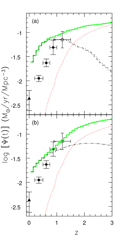
Figure 12: Comoving volume star-formation rate density $\Psi(t)$ as a function of redshift for field galaxies. The contribution of late-types to the cosmic SFR (dot dashed line) derived from our sample is compared in the two cases with the evolutionary path for early-type galaxies studied by FA98 (dotted line). The solid line corresponds to the total amount of SF density in the field. The panels correspond to two different extreme solutions (see text for details): the younger and more extinguished (panel [a]), the older less affected by dust absorption (panel [b]). The data reported are from Lilly et al. (lillyb (1996)) and Connolly et al. (connolly (1997)).

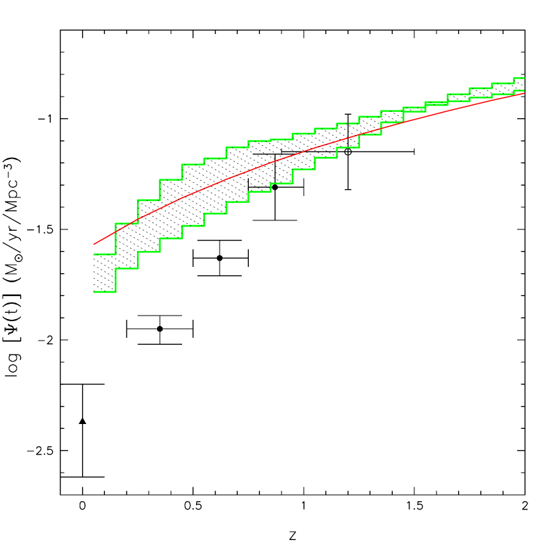
Figure 13: The total star formation rate density per unit comoving volume for field galaxies (late+early-types) is compared with the prediction of Cowie et al. (cowie (1999)), who found a dependence of $\Psi(z)$ on $z$ in the range $0.2<z<1.$ of the form $\Psi(z)\propto(1+z)^{1.5}$ (continous line). The shaded region is bracketed by the two solutions based on the younger-high extinction (upper histogram) and the older less extinguished (lower histogram) models. See also caption to Fig. 12.

The disk–dominated and the irregular galaxies in the present sample display an evolutionary behaviour different from that of bulge–dominated objects. The former appear to form actively stars well below $z=1$, whereas the rate of SF for the latter is high at $z>1$ but converges very fast at lower $z$. Our result for the disk and irregular galaxies is quite consistent with those by Brinchmann et al. (brinchmann (1998), their fig. 15), in showing a comoving SFR modestly increasing between $z=0.3$ and 1. On the contrary, our results differ significantly from Brinchmann et al. as far as the early-type systems are considered (in their case E/S0 have a flat $\Psi(t)$ in the same z-interval): we explain this as due to the very different procedures adopted to measure the function $\Psi(z)$, in our case it was a global fit to the UV-optical-NIR SED, in their case the use of the OII EW as a tracer of SF. Indeed, the latter should more likely trace a negligible residual of SF due to low-level merging activity or stellar recycling, than the global history of SF in these galaxies.

Note that, despite the large uncertainties on the single object, the overall result is fairly well constrained between the two extreme solutions depicted by the shaded region in Figure 13. This is due to a sort of compensation intervening in the adopted solutions: the younger-more extinguished one tends to have a more intense ongoing SF activity but less protracted in time, while the contrary happens for the older less-extinguished solutions. In other words, the baryonic mass already converted into stars and sampled by the near-IR (JHK) flux measurements as a function of redshift, provides a more robust evaluation of the evolutionary SFR than the instantaneous SFR mapped by the short-wavelength flux. In a sense, the errorbar appearing in Fig. 11 does not translates into a similarly large uncertainty in the prediction of Fig. 13, because the ongoing rate of SF (SFR in panel [a] of Fig. 11) and the timescale of SF ($M_{tot}/SFR$ in panel [c]) scale inversely to the galaxy mass function observed at various redshifts.

This prompted us to compare our results with those published by Cowie et al. (cowie (1999)). This is done in Figure 13 where our results appear as the shaded region, which is bracketed by the two solutions based on the younger-high extinction (upper histogram) and the older less extinguished (lower histogram) models. The continuous line is a polynomial function [$\Psi(z)\propto(1+z)^{1.4}$] quoted by Cowie et al. (cowie (1999)) as best-fitting their and Treyer’s et al. (treyer (1998)) data on the time-dependent UV luminosity density. Within the uncertainties, our results are in quite better consistency with the Cowie et al. (1999) evolutionary law than with the dataset compiled by Madau et al. (madau (1996)), based on the CFRS (Lilly et al. lillyb (1996)) and the low-z H_α survey by Gallego et al. (gallego (1995)).

While some discussions can be found in Cowie et al. (cowie (1999)) about possible origins for this discrepancy and on the consequences on this new evaluation of the evolutionary SFR, we only take note here of the nice agreement between our results and those of Cowie et al. (cowie (1999)), based on quite indipendent grounds.

It is remarkable that UV and near IR selected galaxy samples show such similar evolution of the comoving SFR density $\Psi(z)$.

5 DISCUSSION AND CONCLUSIONS

With the main goal to investigate systematic differences between early-type and late-type galaxies – as for colours, redshift distributions, and ages of the dominant stellar populations – we have analyzed a morphologically-selected complete sample of 52 spiral and irregular galaxies in the Hubble Deep Field North with total K-magnitudes brighter than K=20.47 and typical redshifts from $z\sim 0.5$ to 1.5. The sample makes use of total photometry in the UBVI bands from HST and the JHK bands from ground, all carefully tested with an extensive set of Monte Carlo simulations.

The present sample exploits in particular the ultimate imaging quality achieved by HST in this field, allowing us to disentangle among galaxy morphologies, based on accurate profiles of the surface brightness distributions.

Our analysis makes also use of an exhaustive set of modellistic spectra accounting for a variety of physical and geometrical situations for the stellar populations, the dusty ISM, and relative assemblies. The high photometric quality and wide spectral coverage allowed us to estimate accurate photometric redshifts for 16 objects lacking a spectroscopic measurement.

We have also carefully evaluated all plausible systematic effects of the selection, in particular the redshift cutoff implied by the limiting surface-brightness achievable in the reference K band image.

A warning is in order, in any case, about the general conclusions derived from our sample of K-selected galaxies: they should be treated with caution, due to the very small field of view and modest spatial sampling of the present survey. Ferguson et al. (2000) and Eisenhardt et al. (2000) estimate that the number of $L^{*}$ galaxies in the total HDF co-moving volume between z=1 and z=2 is only a few dozens. Considering also the strong clustering inferred for Lyman break galaxies (Adelberger et al. 1998), statistical fluctuations imply large uncertainties on any conclusions based on samples like the HDF, untill more substantial surveys to similar depths will be made available.

Three the main results of our study.

• The sample galaxies are distributed in redshift up to $z=1.4$, but appear to be significantly missing above, compared with evolutionary models assuming standard recipes for the luminosity evolution and a substantial redshift of formation. We reported a similar finding in our previous study of early-type galaxies in the same area (Franceschini et al. 1998). Our conclusion is that, either the area has some peculiarities, or the underlying mass function for galaxies of all morphological kinds has a global decline at these high redshifts. Confirmation of this result will require more substantial sky areas to be surveyed to similar depths by large telescopes.

• Differences between early- and late-types are apparent in the rest-frame colour distributions and the evolutionary star-formation rates per unit volume. In particular, the short-wavelength rest-frame colours B-J, once dust reddening is taken into account, appear quite significantly bluer for late- than for early- galaxy types. On the contrary, the longer-wavelength colors V-K appear to be very similar for the two morphological classes. We interprete this as an indication that, while the stellar mix in spirals/irregulars includes young newly formed populations, less apparent in E/S0, the underlying older age component traced by the V-K colors has quite a similar origin and age distribution for the two galaxy categories.

  We warn, however, that the complication in spectro-photometric modelling introduced by dust-extinction in the gas-rich systems prevents to reach conclusive results on the source by source basis. Only future long-wavelength IR observations, from space (SIRTF, FIRST, NGST) and from ground (10 m class telescopes in the mid-IR and interferometers in the sub-mm), will allow to break down the age/extinction degeneracy.

• We found that an integrated quantity like the comoving-volume star-formation rate density as a function of redshift $\Psi(z)$ is much less affected by the uncertainties related to the dust distribution. The reason for this is mostly in the fact that our analysis is strongly constrained by the evolutionary baryonic mass function in stars traced by the near-IR galaxy luminosities, the estimate of the baryon mass at any redshifts being much more robust than that of the instantaneous rate of star formation (see Sect. 4.5).

  By combining this with the early-type galaxy sample previously studied by FA98, we find a shallower dependence of $\Psi(z)$ on $z$ between $z=0.2$ and $z=1.5$ than found by Lilly et al. (1996), i.e. $\Psi(z)\propto(1+z)^{1.4}$ rathen than $\Psi(z)\propto(1+z)^{4}$ as in Lilly et al. (lillyb (1996)). In this redshift interval our observed $\Psi(z)$ turns out to roughly agree with results published by Cowie et al. (cowie (1999)) and Treyer et al. (treyer (1998)).

  Our present results, based for the first time on a careful modelling of the whole UV-optical-NIR Spectral Energy Distributions of galaxies, then support a revision of the Lilly-Madau plot at low-redshifts for UV- and K-band selected galaxies. UV-selected and near infrared selected galaxy samples display a remarkably similar evolution of the comoving SFR density $\Psi(z)$, at $z<1$.

The three above findings seem to favour the general scheme of hierarchical assembly for the formation of bright galaxies, envisaging their progressive build up during a substantial fraction of the Hubble time. After all, this is the most physically motivated present description.

In this context, a warning is in order concerning some published specializations of the Cold Dark Matter cosmogonic scheme, predicting that spheroidal galaxies in the field form at low redshift ($z<1$) from merging of spirals (Kauffmann & Charlot kauffmannb (1998)). This prediction is not supported by our results in Fig. 12, where Ellipticals and S0s appear to have been mostly formed at $z=1$, whereas spirals/irregulars keep some sustained SF activity at $z<1$. This result suggests that merging of spirals to form ellipticals at low redshifts cannot be a dominant process, quite in agreement with what found by Brinchmann & Ellis (brinchmannb (1998)).

It is conceivable, however, that minor modifications of the CDM hierachical scheme (e.g. in terms of different assumptions about the cosmological parameters $\Omega_{m}$, $\Omega_{\Lambda}$) can explain the observed differences between morphological types. In our view, these differences in the population histories are quite probably related to the presence of different environments at different densities (and consequently different cosmic timescales of formation) in what we call the ”field”. In particular, moderately high-density environments (typically galaxy groups, as found very numerous in the spectroscopic survey by Cohen et al. cohenb (1999)), with an accelerated cosmic timescale of evolution and fast gas consumption, mix with truly low-density environments, where the transformation of primordial gas into stars slowly progresses during the whole Hubble time. We believe that the two galaxy morphologies analyzed in the present paper and in FA98 trace such different environments in the universe.

Table 1: Photometric data on the sample galaxies

id	$\alpha$	$\delta$		$r_{e}(")$	$U_{AB}$	$B_{AB}$	$V_{AB}$	$I_{AB}$	$J_{corr}$	$H_{corr}$	$K_{corr}$	$z$	$A_{V}$	$M_{tot}$	SFR
	$s$	′	′′
0	56.65	12	45.60	1.21	24.91	22.49	21.09	20.05	18.26	17.48	16.79	0.517	0.17	2.97	6.61
1	51.08	13	20.73	1.12	21.69	20.52	19.95	19.63	18.40	17.87	17.30	0.199	1.03	0.26	10.73
2	46.15	11	42.05	0.34	23.40	22.90	22.40	20.80	19.17	18.38	17.37	1.012	2.25	18.19	536.4
3	53.90	12	54.05	0.60	23.74	22.80	21.89	20.88	19.12	18.30	17.47	0.642	1.16	2.44	34.28
4	43.96	12	50.13	0.31	23.90	22.87	21.83	21.01	19.27	18.46	17.59	(0.55)	1.74	2.43	33.01
5	44.58	13	4.66	0.54	25.24	23.63	22.23	21.24	19.29	18.40	17.67	(0.68)	1.15	2.31	27.18
6	51.78	13	53.73	0.49	23.92	22.97	21.97	21.09	19.42	18.51	17.70	0.557	1.56	1.99	27.12
7	42.91	12	16.26	0.52	22.86	22.22	21.32	20.74	19.20	18.53	17.90	0.454	0.28	0.56	7.58
8	49.75	13	13.09	0.63	24.99	23.54	22.29	21.49	19.07	18.56	18.00	0.478	1.34	1.07	11.17
9	50.25	12	39.72	0.49	22.59	22.08	21.25	20.69	19.3	18.67	18.00	0.474	0.37	0.39	10.73
10	41.95	12	5.41	0.47	23.34	22.60	21.67	21.03	19.42	18.78	18.04	0.432	0.34	0.40	4.88
11	45.85	13	25.81	0.85	23.23	22.30	21.45	20.95	19.45	18.86	18.13	(0.4)	0.48	0.38	6.92
12	43.18	11	48.05	0.47	26.05	24.95	23.91	22.45	20.14	19.29	18.23	(1.06)	0.89	3.47	26.09
13	51.72	12	20.18	0.34	24.85	23.34	22.24	21.55	19.87	19.12	18.31	0.299	0.95	0.17	1.57
14	42.72	13	7.26	0.33	25.61	24.58	23.22	22.19	20.00	19.21	18.32	(0.737)	1.73	2.83	32.42
15	47.04	12	34.96	0.40	22.84	22.19	21.46	21.03	19.66	19.05	18.34	0.321	1.00	0.22	7.45
16	49.51	14	6.77	0.34	24.17	23.58	22.82	21.83	20.17	19.23	18.41	0.752	2.07	2.93	67.43
17	49.51	12	20.11	0.61	25.58	25.16	24.04	22.46	20.34	19.40	18.53	0.961	1.03	2.55	22.83
18	41.42	11	42.89	0.33	26.18	25.13	24.81	24.16	20.69	19.66	18.60	1.320	1.03	1.58	16.88
19	58.76	12	52.35	0.85	23.18	22.52	21.72	21.31	19.92	19.34	18.77	0.320	0.38	0.08	2.72
20	55.58	12	45.43	0.47	24.18	23.63	22.97	21.97	20.35	19.65	18.86	0.790	0.70	0.92	17.98
21	50.47	13	16.16	0.64	25.46	24.62	23.74	22.60	20.68	19.95	18.90	(0.88)	1.65	1.05	14.25
22	57.33	12	59.63	0.44	22.83	22.53	21.82	21.38	20.10	19.42	18.93	0.473	0.47	0.15	8.25
23	41.31	11	40.87	0.33	27.02	24.70	23.61	22.47	20.57	19.73	19.01	0.585	0.67	0.51	2.75
24	38.44	12	31.35	0.59	26.76	25.15	23.74	22.67	20.85	20.03	19.17	(0.7)	1.06	0.49	6.90
25	49.24	11	48.38	0.32	25.46	24.93	24.16	22.96	20.67	19.98	19.18	0.961	0.23	1.03	7.75
26	48.62	12	15.81	0.47	26.70	26.20	25.20	23.60	21.23	20.23	19.21	(1.35)	0.96	2.95	14.55
27	49.45	13	16.58	0.28	25.41	24.44	24.02	23.27	21.18	20.22	19.22	(1.006)	1.74	2.55	40.67
28	48.12	12	14.90	0.88	24.26	23.83	23.54	22.64	20.53	20.02	19.36	0.961	0.27	0.90	11.62
29	54.10	13	54.35	0.45	24.35	23.84	23.37	22.43	21.01	20.17	19.41	0.894	1.68	1.37	46.13
30	52.70	13	55.49	0.27	23.96	23.22	23.06	22.71	20.64	20.08	19.41	1.355	0.54	0.67	44.33
31	38.99	12	19.63	0.45	24.14	23.67	22.95	22.22	20.81	20.17	19.57	(0.77)	1.51	1.07	53.23
32	44.19	12	47.90	0.39	22.99	22.65	22.13	21.65	20.50	19.91	19.58	.558	0.50	0.27	11.04
33	49.01	12	20.86	0.18	23.87	23.54	23.23	22.44	20.89	20.53	19.68	0.953	0.47	0.34	18.31
34	39.56	12	13.83	0.44	28.20	26.49	25.15	23.79	21.62	20.53	19.69	(1.22)	2.07	3.48	62.76
35	48.27	13	13.8	0.29	26.53	25.90	25.30	24.07	21.51	20.36	19.75	(1.165)	0.57	1.15	9.37
36	53.45	12	34.52	0.34	24.97	24.25	23.50	22.81	21.47	20.83	19.80	0.559	2.08	0.41	15.00
37	55.53	13	53.48	0.70	24.04	23.49	23.23	22.65	21.27	20.48	19.80	1.148	1.70	2.19	108.8
38	49.58	14	14.63	0.48	25.40	24.00	23.80	22.70	21.37	20.75	19.94	(0.92)	0.82	0.30	22.39
39	57.67	13	15.32	0.39	24.43	23.94	23.57	22.82	21.29	20.71	19.97	0.952	0.46	0.31	14.37
40	55.50	14	2.71	0.55	26.06	24.87	23.87	22.99	21.48	20.75	20.01	0.559	1.07	0.16	3.66
41	48.79	13	18.35	0.68	24.27	23.93	23.50	22.76	21.32	20.27	19.66	0.749	1.85	0.30	25.12
42	47.19	14	14.18	0.22	26.70	25.74	24.59	23.53	21.84	20.63	20.02	0.609	1.83	0.40	5.10
43	57.21	12	25.83	0.51	24.17	24.02	23.91	22.45	21.34	20.60	20.05	0.561	0.32	0.11	2.21
44	48.34	14	16.63	0.16	25.86	23.97	23.73	23.43	21.64	20.53	20.11	2.008	0.33	1.69	51.3
45	47.78	12	32.93	0.28	25.21	24.73	24.27	23.34	21.47	21.12	20.12	(1.04)	0.98	0.64	22.47
46	52.87	14	5.11	0.29	25.70	24.84	24.06	23.25	21.38	20.89	20.21	0.498	0.16	0.08	0.57
47	52.02	14	0.91	0.33	25.25	24.55	23.72	23.02	21.48	20.74	20.22	0.557	0.23	0.08	1.26
48	48.58	13	28.35	0.47	25.33	24.30	23.95	23.00	21.22	21.08	20.24	0.958	0.68	0.27	14.77
49	44.64	12	27.39	0.24	25.79	24.28	24.11	23.73	21.63	20.89	20.29	(1.58)	0.18	0.49	14.84
50	44.45	11	41.82	0.62	24.43	24.46	24.52	23.88	21.05	21.25	20.42	1.020	0.17	0.37	4.02
51	56.13	13	29.74	0.39	24.38	24.13	23.97	23.34	21.38	21.30	20.45	(1.2)	0.80	0.72	32.59
41	48.79	13	18.35	0.68	24.27	23.93	23.50	22.76	21.32	20.27	19.66	0.749	1.85	0.30	25.12
42	47.19	14	14.18	0.22	26.70	25.74	24.59	23.53	21.84	20.63	20.02	0.609	1.83	0.40	5.10
43	57.21	12	25.83	0.51	24.17	24.02	23.91	22.45	21.34	20.60	20.05	0.561	0.32	0.11	2.21
44	48.34	14	16.63	0.16	25.86	23.97	23.73	23.43	21.64	20.53	20.11	2.008	0.33	1.69	51.3
45	47.78	12	32.93	0.28	25.21	24.73	24.27	23.34	21.47	21.12	20.12	(1.04)	0.98	0.64	22.47
46	52.87	14	5.11	0.29	25.70	24.84	24.06	23.25	21.38	20.89	20.21	0.498	0.16	0.08	0.57
47	52.02	14	0.91	0.33	25.25	24.55	23.72	23.02	21.48	20.74	20.22	0.557	0.23	0.08	1.26
48	48.58	13	28.35	0.47	25.33	24.30	23.95	23.00	21.22	21.08	20.24	0.958	0.68	0.27	14.77
49	44.64	12	27.39	0.24	25.79	24.28	24.11	23.73	21.63	20.89	20.29	(1.58)	0.18	0.49	14.84
50	44.45	11	41.82	0.62	24.43	24.46	24.52	23.88	21.05	21.25	20.42	1.020	0.17	0.37	4.02
51	56.13	13	29.74	0.39	24.38	24.13	23.97	23.34	21.38	21.30	20.45	(1.2)	0.80	0.72	32.59

References

- (1) Adelberger, K.L., Steidel, C.C., Giavalisco, M., Dickinson, M.E., Pettini, M., Kelog, M. 1998, ApJ 505, 18
- (2) Bertin, E., Arnouts, S., 1996, A&AS 117, 393
- (3) Brinchmann, J., Abraham, D.S., Tresse, L., Ellis, R.S., Lilly, S. et al., 1998, ApJ 499, 112
- (4) Brinchmann, J. and Ellis, 2000, astro-ph/0005120
- (5) Cohen, J.G., Cowie, L.L., Hogg, D.W., Songaila, A., Blandford, R., Hu, E.M., Shopbell, P., 1996, AJ 471, L5
- (6) Cohen, J.G., Blandford, R., Hogg, D.W., Pahre, M.A., Shopbell, P.L., 1999, ApJ 512, 30
- (7) Connolly, A.J., Szalay, A.S., Dickinson, M., Subbarao, M.U., Brunner, R.J., 1997, ApJ 486, L11
- (8) Cowie, L.L., Songaila, A., Barger, A.J., 1999, AJ 118, 603
- (9) Cowie, L.L. et al., 1996, http://www.ifa.hawaii.edu/cowie/hdf.html
- (10) Dickinson, M. et al., 1997, http://archive.stsci.edu/hdf/hdfirim.html
- (11) Eisenhardt, P., Elston, R., Stanford, S.A., Dickinson, M., Spinrad, H., Stern, D., Dey. A., 2000, astro-ph/0002468
- (12) Ellis, R.S., 1997, ARA&A 35, 389
- (13) Fernandez-Soto, A., Lanzetta, K.M., Yahil, A., 1998, http://bat.phys.unsw.edu.au/fsoto/hdf
- (14) Franceschini, A., Silva, L., Fasano, G., Granato, G.L., Bressan, A., Arnouts, S., Danese, L., 1998, ApJ 506, 600
- (15) Gardner, J.P., Sharples, R.M., Frenk, Carrasco, B.E., 1997, ApJ 480, L99
- (16) Gallego, J., Zamorano, J., Aragon-Salamanca, A., Rego, M., 1995, ApJ 455, L1
- (17) Kauffmann, G., Charlot, S., 1998, MNRAS 297, L23
- (18) Lilly, S.J., Tresse, L., Hammer, F., Crampton, D., Le Fevre, O., 1995, ApJ 455, 108
- (19) Lilly, S.J., Le Fevre, O., Hammer, F., Crampton, D., 1996, ApJ 460, L1
- (20) Madau, P., Ferguson, H.C., Dickinson, M.E., Giavalisco, M., Steidel, C.C., Fruchter, A., 1996, MNRAS 283, 1388
- (21) Oke, J.B., Gunn, J.E., 1983, ApJ 266, 713
- (22) Rodighiero, G., Franceschini, A. and Fasano, G., 2000, in preparation
- (23) Silva, L., Granato, G.L., Bressan, A., Danese, L., 1998, ApJ 509, 103
- (24) Treyer, M.A., Ellis, R.S., Milliard, B., Donas, J., Bridges, T.J., 1998, MNRAS 300, 303
- (25) Williams, R.E., Blacker, B., Dickinson, M., Dixon, W.V., Ferguson, H.C. et al., 1996, AJ 112, 1335
- (26) Wolfe, A.M., 1999, American Astronomical Society, Meeting 194, #63.07