High Speed Phase-Resolved 2-d $UBV$ Photometry of the Crab pulsar

Abstract

We report a phase-resolved photometric and morphological analysis of $UBV$ data of the Crab pulsar obtained with the 2-d TRIFFID high speed optical photometer mounted on the Russian 6m telescope. By being able to accurately isolate the pulsar from the nebular background at an unprecedented temporal resolution (1 $\mu$s), the various light curve components were accurately fluxed via phase-resolved photometry. Within the $UBV$ range, our datasets are consistent with the existing trends reported elsewhere in the literature. In terms of flux and phase duration, both the peak Full Width Half Maxima and Half Width Half Maxima decrease as a function of photon energy. This is similarly the case for the flux associated with the bridge of emission. Power-law fits to the various light curve components are as follows; $\alpha$ = 0.07 $\pm$ 0.19 (peak 1) , $\alpha$ = -0.06 $\pm$ 0.19 (peak 2) and $\alpha$ = -0.44 $\pm$ 0.19 (bridge) - the uncertainty here being dominated by the integrated CCD photometry used to independently reference the TRIFFID data. Temporally, the main peaks are coincident to $\leq$ 10 $\mu$s although an accurate phase lag with respect to the radio main peak is compromised by radio timing uncertainties. The plateau on the Crab’s main peak was definitively determined to be $\leq$ 55 $\mu$s in extent and may decrease as a function of photon energy. There is no evidence for non-stochastic activity over the light curves or within various phase regions, nor is there evidence of anything akin to the giant pulses noted in the radio. Finally, there is no evidence to support the existence of a reported 60 second modulation suggested to be as a consequence of free precession.

1 Introduction

As the youngest known isolated rotation powered neutron star, and having the highest known spin-down flux density, the Crab pulsar is not surprisingly the most efficient source of high energy magnetospheric emission. All theoretical models attempting to elucidate the processes of nonthermal emission must satisfy the empirical constraints provided by the extensive observational datasets available for this object from $\gamma$-rays to the infrared.

Contemporary theoretical frameworks in existence to explain the nonthermal emission from this and other isolated rotation-powered neutron stars may be broadly divided into two schools. The first places the source of emission close to the polar cap region, e.g. Sturrock (1971), and the second that place the source at a considerable distance above the neutron star surface, in the outer magnetosphere (e.g. Cheng, Ho & Ruderman 1986). In recent times, the development of these models has been to some extent restricted to the problem of $\gamma$-ray emission. These efforts have been predominantly analytical in nature, as in this energy regime primary emission is being sampled, which avoids complications associated with the lower energy sources of emission. In these latter cases, the emission is secondary in nature and a result of interactions that require numerical representation. Thus the polar cap school (e.g. Daugherty & Harding 1982) concluded with correct flux estimates but poor light curves, and the outer gap school (Cheng, Ho & Ruderman 1986) with reasonable light curves and approximate flux distributions but requiring extraordinary lines-of-sights and magnetospheric physics to justify the emission.

The group at Stanford University lead by R. Romani is generally credited by being the first to rigourously put the existing models to the test numerically. Their conclusions in many ways matched the intuitive premonitions regarding the two model frameworks, with perhaps the ‘evolved’ outer gap model of Cheng, Ho & Ruderman (1986) being the more likely candidate (Chiang & Romani 1992; Romani & Yadagiroglu 1995). Recently Romani (1998) has indicated that it is only by both the development of more advanced numerical simulations that incorporate the full emission physics (from $\gamma$-rays to the IR) in a truly self-consistent manner and the accurate characterisation of pulsar light curves in the lower energy regimes that one can hope to disentangle the problem of nonthermal pulsar emission.

Optically, spectroscopic, integrated and high speed single-pixel photometry have produced some critically important results in this regard. However, true phase-resolved data acquisition with accurate isolation of the pulsar’s emission from that of the nebula requires high time resolved ($\sim$ 1 $\mu$s) 2-d photometry to confirm unambiguously earlier conclusions and to determine the true nature of the magnetosphere’s emission in the range $\sim$ 1 - 10 eV.

In a previous paper (Golden et al. 2000), we presented an analysis of such observations of the Crab pulsar in which we isolated and theoretically speculated upon the unpulsed component of the pulsar’s optical emission. These observations were made in January 1996 with the TRIFFID 2-d high speed photometer in three colourbands ($UBV$) using the 6m BTA of the Special Astrophysical Observatory in the Russian Caucasus. Here we present a thorough photometric and temporal analysis of the same data. Following a review of the pulsar’s relevant empirical and theoretical characteristics, we briefly outline the observational and data reduction methodology - the reader is encouraged to consult Golden et al. (2000) for a more rigorous treatment of this process. We then detail the results of the photometric and temporal analysis, and conclude with a discussion on the implications of these results for current thinking on this pulsar, with wider ramifications for pulsar emission theory in general.

2 Review

The Crab pulsar is identified as the south-west member of the double stars located in the central region of the Crab Nebula (Cocke et al. 1969). Radio observations, initially by Staelin $\&$ Reifenstein (1968), and regularly ever since, have provided perhaps one of the most detailed pulsar rotational datasets to date. The pulsar has a $P$ $\sim$ 33 ms and $\dot{P}$ $\sim$ 4.211$\times 10^{-13}$ s$\rm s^{-1}$ suggesting a canonical age of $\tau$ $\sim$ 1260 years and surface magnetic field $B_{surface}$ $\sim$ 3.7 $\times 10^{12}$ Gauss.

Historically, high speed optical photometry has been generally dominated by the use of single pixel detectors, with variable time resolution. Following the detection of Cocke et al. (1969), numerous targetted observations followed (Kristian et al. 1970; Wampler et al. 1969; Warner et al. 1969; Becklin et al., 1973; Muncaster and Cocke, 1972; Cocke and Ferguson 1974; Groth 1975a,b) with the pulsar generally observed in the $BVRI$ wavebands at typical accurate time resolutions of order $\sim$ ms, and the datasets ‘added’ together in a least-squares fashion - there being no common stabilised ‘clock’ from which to time the observations, nor a definitive radio ephemeris with which to accurately obtain in modulo lightcurves at that time.

The development of more ”temporally consistent” instrumentation in conjunction with other advances in technology allowed for more detailed observations to be taken. Peterson et al. (1978) applied for the time rather novel techniques in the image processing of data obtained via the use of a 6.2 ms time resolved 2-dimensional Image Photon Counting System camera. Significant emission from the unpulsed presumed ‘off’ component was noted in the $U$ and $B$ bands, with Peterson et al. estimating that it was some 2% of the total pulsed emission.

At an effective time resolution of 20 $\mu$s, Smith et al. (1978) were able to make unprecedented observations via a S20 photocathode of the Crab’s main pulse region, indicating that the peak had a plateau of emission $\leq$ 100 $\mu$s in duration. Photon binning at 1 kHz allowed for phase resolved tests to be made of the counting statistics incident on the detector. They yielded statistical distributions that did not deviate significantly from random fluctuations expected, making an allowance for variations in sky transparancy.

Subsequent high speed observations incorporating an appropriate polarisation set-up yielded phase resolved polarimetry (Jones et al. 1981, Smith et al. 1988). Under analysis and corrected for interstellar polarisation, these datasets show evidence for sharp swings in polarisation angle around both principle peaks, in addition to some form of evolution of the polarisation in the bridge area. Remarkably, the results indicated substantial polarisation associated with what was always assumed to be ‘off’ or at the very least, the pulsar at a minimum, as noted earlier by Peterson et al. (1978).

The High Speed Photometer (HSP) on board the Hubble Space Telescope ($HST$) was used to observe the Crab pulsar in October 1991 and again in January 1992, as reported by Percival et al. (1993). The passbands used were F400LP and F160LP, which crudely approximate to standard $V$ and $UV$. Although the on-board clock is accurate to 10.74 $\mu$s, accuracy to UTC was typically $\sim$ $\pm$ 1.05 ms per observing run. Each resulting light curve had an effective temporal resolution of 21.5 $\mu$s.

The pertinent results of Percival et al. (1993) are as follows. They estimated that the main pulse in the visible leads the radio by -1.47 $\pm$ 1.05 ms, and for the UV, -0.91 $\pm$ 1.05 ms, with both $UV$ and $V$ main peaks offset by 0.56 $\pm$ 0.92 ms. Via autocorrelation and least-squares analysis of the light curves, the Full Width Half Maximum (FWHM), peak separation and peak ratios were determined. Despite the summing and normalising of the individual light curves which might be expected to introduce an element of bias in any analysis, Percival et al. (1993) obtain consistent and reasonable estimates for these parameters. The implication is that there is a trend whereby the pulse peaks ‘tighten’ and come together as a function of energy. Resolution of the main peak cusp was attempted via a least-squares polynomial fit, and was found to be $\leq$ 150 $\mu$s in extent. Despite a number of caveats outlined previously Percival et al. (1993) can claim to have shown to a reasonable degree that

1. The peaks’ FWHM and separation contract as a function of energy.

2. The $UV$ and $V$ main peaks appear to be coincident to within $\sim$ 1 ms.

3. The $UV$ and $V$ main peaks show signs of leading the radio main peak.

4. A plateau of emission is not definitively resolvable to within 150 $\mu$s.

5. The photon statistics would appear to be Poissonian throughout the light curve.

Later observations, using the $HSP$ in Polarisation mode, were made of the pulsar (Smith et al. 1996). Qualitatively the results were similar to earlier optical observations. The conlusions reached were no different to the original 1988 paper, other than that any model of the emission regions must be essentially wavelength independent.

Following on from $IR$ band observations of Ransom et al. (1994), Eikenberry et al. (1996) made observations in the $J$, $H$ and $K$ bands using a single-pixel Solid State Photomultiplier, set-up to record using 20 $\mu$s time bins. Light curves were then obtained in the usual manner.

The analysis proceeded along three avenues. The first was determination of the Half Width Half Maximum (HWHM), essentially a truncated FWHM, with each side of the FWHM bisected by the maximum of the peak in question, yielding a ‘leading’ and ‘trailing’ HWHM component. The second was the determination of phase resolved spectra, and the third an in-depth examination of the colour variation around the main peak. Monte Carlo simulations were used to build up a statistical picture of the optimum fits to the light curve data.

This analysis showed clear evidence that the peaks (morphologically and in terms of flux) change as a function of energy throughout the light curve, and also that time limit over which such rapid spectral changes occured was $\leq$ 180 $\mu$s. Assuming emission occurs in the vicinity of the light cylinder, then one can estimate the typical coherence dimensions for the region, being less than or equal to 1.8 $\times 10^{-4}$ s $\times$ $c$ = 54km - indicating that the emission region is consistent with a localised region of the magnetosphere.

In a subsequent paper (Eikenberry & Fazio 1997) these techniques were applied to a range of light curves, from $\gamma$-rays (Ulmer et al. 1995), X-rays (reconstructed from the $ROSAT$ archives), $UV/V$ (Percival et al. 1993) and $KHJ$ (from previous work). The overall energy range spanned 0.47 eV to 10 MeV. The principle intention was to further test the hypothesis that the actual peaks themselves altered morphologically with energy. The actual mechanics of how the datasets were analyzed was similar to the earlier analysis of Eikenberry et al. (1996) - it will suffice to note their more pertinent conclusions;

1. The ratios of the flux of the bridge and peak 2 to peak 1 show an overall trend to increase with energy, but reverses at low energies ( $<$ 1eV ).

2. The peak-to-peak separation shows a ‘nonlinear’ trend to decrease with energy over the range, which is consistent with energy stratification of the emission region.

3. The peaks FWHM show neither a definite trend nor pattern with energy, yet display significant variability over the range.

4. There is a strong energy dependency as regards the evolution of the HWHM for leading and trailing edges of both peaks, with some evidence of a continous functionality over the range - except at the $IR$ region. The HWHM behaviour explains the rather puzzling FWHM behaviour.

5. Peak 2 appears to change profoundly as regards morphology between the $IR$-optical and X-ray-$\gamma$-ray range, showing a fast rise and slow fall for the former, and the converse for the latter. This is not explicable by theory.

6. Many of the pulse shape parameters show maxima or minima at the energies of 0.5-1eV in the $IR$ regime, suggesting some interesting phenomena occuring in this waveband.

Eikenberry & Fazio (1997) concluded that the many unusual energy dependent morphological phenomena that are observed under this analysis were incompatible with current model frameworks - in particular the single-pole emitting outer-gap (Romani & Yadigaroglu 1995). In this model, the emission originates from a topologically extended region that effectively maps out a hemisphere about the open field region. Consequently, with the emission profile a result of viewing geometry and crossing caustics to the line of sight, one would expect either no evident effect, or a common effect that should manifest itself in a smooth and continuous manner at all such energies, as the effect would be essentially the averaging of many seperate spatially emission sources. These expectations contrast with the empirically determined results.

3 Precession Issues

Free precession of an isolated pulsar, most likely due to some moment of inertia inequality, possibly as a result of irregular distributions of neutron star matter on its surface, or perhaps as a result of internal interactions and effects, would manifest itself as an appropriate modulation in the observed temporal signal. Previous reports by groups examining the variations in the ratios of peak 1 to peak 2 in $\gamma$-rays have generally indicated periods of the order of years (Kanbach et al. 1990; Nolan et al. 1993; Ulmer et al. (1994). Previous reports of something akin to a precessional like signal from the Crab pulsar in the radio have tended to suggest a precessional period of order months/years (e.g. Jones 1988).

At higher frequencies, evidence of precession could provide both direct constraints to the condensed matter equation of state, and imply the emission of gravitational radiation. It is well known that a precessing gravitationally compact body rotating at high speeds would be expected to radiate gravity waves, at a frequency twice its rotational frequency (e.g. Misner, Thorne & Wheeler, 1971). Various other emission modes are theoretically possible. Planned ground based gravitational detectors are being designed that could have the capability to detect displacement amplitudes of order $h$ $\sim$ $10^{-23}$. However do this, these detectors must be ‘tuned’ to a particular tight frequency band for up to 1 year to build up sufficient $S/N$. Clearly, one needs a guaranteed signal to lock on to - and pulsars may very well provide such a source.

Hence the great interest in the reported suggestions of a precession signal with a period of order 60 seconds from the Crab by Cadez and Galicic (1996). This was based on a time-series analysis of the High Speed Photometer data of Percival et al. (1993), and their own ground based observational CCD dataset. Despite nearly three decades of radio observations, no such modulation has been reported in the literature. Furthermore, an analysis of high speed optical data by Jones et al. (1980) with early photometers indicated a lack of optical source variations at the 1 % level over a ten year period. It is clearly important to try and test this with independent data, as a confirmation would have important possible implications for other fields, particularly that of gravitational wave detection.

4 January 1996 BTA Run - Observations in $UBV$ $\&$ Data Preparation

The details of these TRIFFID high speed observations of the Crab pulsar, and the subsequent preliminary analysis have been published elsewhere (Golden et al. 2000). We shall thus limit our description accordingly. The observations took place over 5 nights in January 1996 using the Special Astrophysical Observatory’s 6m telescope in the Caucasus. TRIFFID high speed camera used incorporated a 2-dimensional photon counting MAMA detector (Cullum (1990); Timothy & Bybee (1985)) with standard $U$, $B$ and $V$ filters. Timing was accurate to within 400 ns per 10 second period using a GPS receiver. There were 6 $U$ band exposures totalling 5546 seconds, 5 $B$ band exposures totalling 5750 seconds, and 9 $V$ band exposures totalling 6759 seconds.

The photon [x,y,t] data stream per dataset was corrected via a Weiner filter modified shift-and-add algorithm for telescope wobble and gear drift (Redfern et al. 1993). Processing the datasets in this way and incorporating the derived flat fields yielded full field images of the inner Crab nebula from which the pulsar and its stellar companions were registered. Figure 1 shows the integrated 96zs2.0.0 dataset following this technique. The average seeing for this dataset was $\sim$ 1.3$\arcsec$. The Crab pulsar is evident as the slightly dimmer upper component of the central double star.

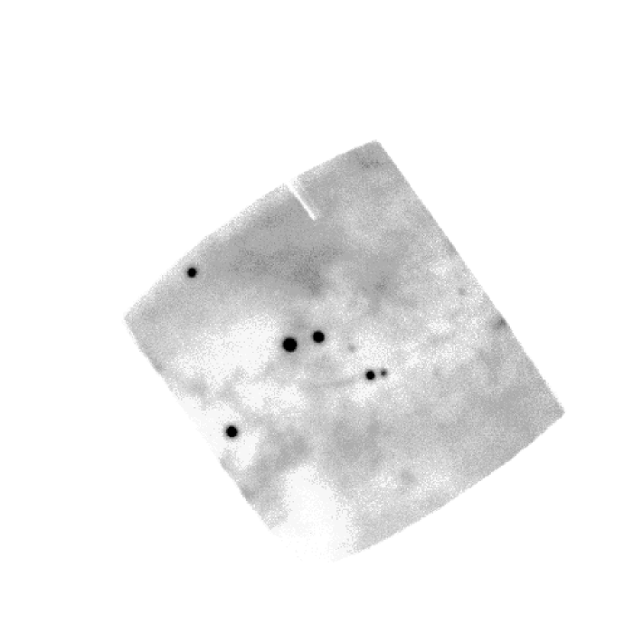
Figure 1: Corrected integrated image for the 96zs2 dataset, in the $V$ band. The consequent effect of a dead anode line is visible in the upper part of the image. The Crab is the fainter of the two centre-left stars.

As detailed in Golden et al. (2000), phase resolved images were obtained by firstly extracting all photons with a fixed pixel radius of the Crab pulsar, barycentering them, and then geometrically aligning each dataset in [x,y] per colour band. This yielded a sequence of time-series per colour band that, when read by a modified epoch-folding algorithm, generated both standard light curves and phase-resolved 2-dimensional image within a certain specified phase range. The latter used the appropriate data taken from the Jodrell Bank Crab Ephemeris (Lyne & Pritchard, 1996).

5 Analysis - Temporal Issues

It is absolutely crucial in this analysis to ascertain the temporal quality of our datasets, and in this way, test for possible glitches in the calibrated timing hardware and potential nonlinearities caused as a result of microchannel plate saturation, thus assessing any unusual temporal activity in the pulsar time series.

Regarding the problem of $MAMA$ saturation it was determined that, within the bounds of variable sky transparancy, no non-Poisson behaviour at the 99% level was noted, for a range of datasets over the $UBV$ wavebands (Golden 1999). This was repeated throughout the light curve, indicating that the emission process is consistent with dominant incoherent synchrotron processes. Giant radio pulses, which are of order 10³ times more intense than the average radio pulse, occur in approximately 1 % of radio pulse periods (Lundgren et al. 1994). There were no deviations in the photon statistics accumulated in these observations consistent with such giant pulse activity.

Regarding the temporal stability of the timing system, we previously determined the timing accuracy to within $\sim$ 1 $\mu$s of UTC, and for long (4-5 days) timeseries datasets, it is possible to test the timing against the Crab pulsar itself via epoch folding or Fourier methods. For the former case, this will be as accurate as the timing ephemeris provided - during our observing period the Jodrell Ephemeris was accurate to 50 $\mu$s. In the latter, we are restricted to the accuracy with which one can determine to have detected a harmonic at high $\nu$. Via epoch folding, the best reduced $\chi^{2}$ was determined for the given rotational parameters from Jodrell within 100 $\mu$s of the given reference time stamp given by the GPS system. Using an Origin2000 supercomputer, detection of the high harmonics (typically $\sim$ 50) for several daily $B$ datasets yielded frequency estimates that were accurate to the corrected ephemeris frequency to within 1 in 10⁷. Consequently, we were satisfied with the temporal integrity of these MAMA datasets taken in Russia in January 1996.

In this vein, the unusual low frequency signal of $\sim$ 0.016 Hz reported by Cadez & Galicic (1996) was put to the test. FFT analysis on each night’s dataset binned at 1, 0.1 & 0.2 Hz were tested, but no significant signal was apparent within the 0.01 - 1 Hz window - or at greater frequencies. Consequently we must remain somewhat guarded as regards the conclusions of Cadez & Galicic (1996). The definitive discovery of a 60 second precessional signal from an isolated rotating neutron star would have profound implications for fundamental physics and thus demands conclusive and undeniable evidence for its justification. We must state that we see no such evidence to date.

6 Analyses - Phase Resolved Photometry

By the use of developed epoch folding algorithms, it was possible to take the deep summed time series for all three wavebands and re-construct a phase-resolved image for a specific phase region. Figure 2 shows such an ad hoc mosaic of phase-resolved images, with the phase resolution here 0.05 of phase.

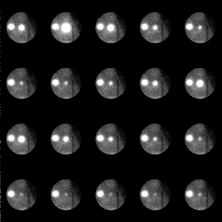
Figure 2: Mosaic image of one cycle in $V$ of the Crab Pulsar. The sequence of phase-resolved frames starts at the top left. To ‘read’ the frames, one moves from left to right along each row. This continues until one reaches the bottom right frame. Thus one can see the main peak initially, the bridge of emission (row 2), the interpulse/peak 2 (end of row 2, row 3), and the ‘off’ phase (row 4). The structure on the right hand side is the dead anode line as seen in Figure 1, and its location in proximity to the pulsar occurred in only one dataset.

It is apparent that there appears to be residual emission from the Crab pulsar during the traditional ‘off’ phase (essentially row 4 in Figure 2), as was originally noted by Peterson et al. (1978). The fact that we can obtain deep phase-resolved images which have been corrected for telescope drift and wobble with a sufficient field of view enables us to rigorously characterise the time-resolved nature of the pulsar’s emission via standard image processing techniques.

There are a number of ways to proceed with this analysis. Principally, we wish to determine 1) what the total background is in a given aperture per colour band and 2) what are the respective fluxes for phase-resolved components of emission associated with the Crab pulsar. The first step is perhaps the most important as it may then be applied to the standard derived light curves so as to correct for the background per bin and thus allow one to characterise the so-called ‘steady’ or ‘off’ phase of emission.

In Golden et al. (2000), the image processing techniques were outlined in some considerable detail for this analysis. It is sufficient to state that the IRAF daophot package was used to remove the full Crab image (and thus obtain the background per aperture per colour band in addition to the full Crab flux), and similarly for the various phase-resolved light curve components, which are localised in terms of phase in Table 1. This process involved the empirical fitting of a PSF to the Crab and making the subsequent extraction.

Table 1: Pulse Phase Definitions.

Phase	Region
Peak 1	-0.12 - 0.12
Peak 1 (Leading Edge)	-0.12 - 0.0
Peak 1 (Trailing Edge)	0.01 - 0.12
Bridge	0.121 - 0.27
Peak 2	0.271 - 0.658
Peak2 (Leading Edge)	0.271 - 0.409
Peak2 (Trailing Edge)	0.410 - 0.658
Off Phase	0.75 - 0.825

The ‘off’ phase here was localised in the following manner. Correcting for the estimated background above, the ‘off’ regions for the various coloured light curves at 11 $\mu$s resolution (3000 bins) were tested via a $\chi^{2}$ algorithm. Here, the bin region was iteratively reduced, and tested to see if the observed flux was consistent with that expected from a non-varying source over that phase region, at the 95 % level.

As regards any nebular contribution to this photometric analysis, no significant change was noted between the estimated flux of the ‘off phase’ made via extraction using the full cycle PSF, and the flux determined by empirically fitting a PSF to the ‘off phase’ itself. This indicates that the local nebulosity does not significantly contribute to the determined fluxes in this work.

6.1 Phase Averaged/Integrated Colour Photometry

Actual phase-resolved photometry was done by normalizing the total Crab flux per colour band to a known integrated photometric reference, and then determining the contribution per phase region based on the fractional fluxes estimated for that particular phase-resolved component. The extinction corrected $UBV$ ground-based photometry of Percival et al. (1993) was used as the reference data for this purpose

Table 2 displays the tabulated fractional fluxes estimated following the photometric analysis detailed previously within each colour band - the fluxes were derived via renormalizing the fractional flux with respect to the Percival et al.’s integrated data.

Table 2: Fractional Flux derived from Photometric Analysis.

Parameters		Waveband
	U (mJy)	B (mJy)	V (mJy)
Peak 1	2.0 $\pm$ 0.1	1.9 $\pm$ 0.1	1.9 $\pm$ 0.1
Peak 2	1.1 $\pm$ 0.1	1.1 $\pm$ 0.1	1.1 $\pm$ 0.1
Bridge	0.09 $\pm$ 0.01	0.10 $\pm$ 0.01	0.11 $\pm$ 0.01
Off Phase	0.014 $\pm$ 0.002	0.017 $\pm$ 0.002	0.019 $\pm$ 0.002
P1 (HWHM) Lead	1.1 $\pm$ 0.1	1.2 $\pm$ 0.1	1.1 $\pm$ 0.1
P1 (HWHM) Trail	0.8 $\pm$ 0.1	0.8 $\pm$ 0.1	0.8 $\pm$ 0.1
P2 (HWHM) Lead	0.46 $\pm$ 0.03	0.49 $\pm$ 0.03	0.46 $\pm$ 0.03
P2 (HWHM) Trail	0.59 $\pm$ 0.04	0.65 $\pm$ 0.04	0.65 $\pm$ 0.04

Table 3: Estimated Spectral Power-Laws from Photometric Analysis

Dataset	Power-Law
	$\propto$ $\nu^{\alpha}$
Integrated UV/U/B/V/R	0.11 $\pm$ 0.09
Integrated U/B/V	-0.07 $\pm$ 0.19
Peak 1	0.07 $\pm$ 0.19
Peak 2	-0.06 $\pm$ 0.19
Bridge	-0.44 $\pm$ 0.19
Off	-0.60 $\pm$ 0.37
Peak 1 HWHM (Leading)	-0.15 $\pm$ 0.19
Peak 1 HWHM (Trailing)	-0.11 $\pm$ 0.19
Peak 2 HWHM (Leading)	-0.04 $\pm$ 0.19
Peak 2 HWHM (Trailing)	-0.18 $\pm$ 0.19

In Table 3 the estimated power-law parameter $\alpha$ has been determined via a weighted linear least-squares fit for each individual spectral dataset, with associated errors. We have re-calculated $\alpha$ for the both the full range ($UVUBV$) & $UBV$ ground-based Percival et al. (1993) datasets to compare with the other power-law fits. Included in this Table are power-law fits to the FWHM and HWHM components.

6.2 Phase Resolved Colour Spectra - the Peaks & Bridge

Figure 3 shows as a function of photon energy the spectral forms based on the fluxes of each peak, and to the same scale and the emission from the bridge component.

Figure 3: Phase-resolved Fluxes over $UBV$ for peaks 1 & 2 and the bridge component of emission

It seems clear that certainly as regards the bulk flux from both peaks, that the functional forms, with $\alpha$ $\sim$ 0.07 $\pm$ 0.19 for peak 1 and $\alpha$ $\sim$ -0.06 $\pm$ 0.19 for peak 2, are to first order identical with that reported for the integrated emission, namely a flat power law ($\alpha$ $\sim$ -0.07 for the ground-based $UBV$, $\alpha$ $\sim$ 0.11 for the full ground-based $UVUBV$ Percival et al. (1993) dataset). This is not entirely surprising, as the dominant emission from the pulsar is localised in the peaks, and the fact that both are identical in form suggests a common population of electrons/magnetic field environment/Lorentz factor. Figure 4 substantiates this common source, there being no significant difference between the colour bands evident in these datasets. There appears to be, however, evidence for a somewhat steeper power-law associated with the bridge component of emission ($\alpha$ $\sim$ -0.44 $\pm$ 0.19).

Figure 4: Flux Ratios between peaks 1 & 2 over $UBV$

In Figure 5 the fractional bridge/peak fluxes are shown as a function of photon energy, both suggesting similar functional forms, consolidating the common proportionality between each flux component. This suggests to first order a different population of emitting electrons / magnetic field environment / Lorentz factor in terms of the bridge component than that for the peaks. However it should be stressed that any definitive differing power-law forms are only significant at the 2$\sigma$ level - in this we are at the mercy of the reference data of Percival et al. (1993), where the substantial error component originates. Using other reference data of a higher photometric quality and further observations at other frequency ranges (such as in the $R$) would constrain these fits significantly.

Figure 5: Flux Ratios for peaks 1 & 2 with respect to the bridge emission.

6.3 Phase Resolved Colour Spectra - Leading & Trailing Peak Edges

In Figures 6 & 7 the HWHM flux estimates for both peaks 1 and 2 are shown - here the leading and trailing HWHM fluxes are derived for each peak. It seems clear that the leading & trailing edges for both peaks present spectral forms that are in agreement with each other (see Table 3), although we are somewhat restricted in our analysis by error considerations.

Figure 6: Leading and trailing HWHM Flux Estimates for peak 1

Figure 7: Leading and trailing HWHM Flux Estimates for peak 2

For both cases, we see suggestions for power-laws with decreasing exponents as a function of frequency, although both are consistent with an essentially flat functional form. These results are in agreement with estimates of Eikenberry & Fazio (1997), whose analysis yielded results which incline towards a decrease in flux with increasing photon energy. It is at $JHK$ wavebands that Eikenberry et al. (1996) observed quite profound changes in the overall spectral forms for the leading & trailing edges of both peaks - certainly in the $UBV$ regime, we appear to be sampling similar synchrotron emitting populations.

7 Analyses - Morphological Characteristics

As has been outlined previously, there has not been to date a consistent set of observational datasets that are temporally accurate (to 1 $\mu$s of UTC), and this has to some extent compromised previous efforts. The data taken in January 1996 provides the first such thorough sample, and we consequently first concentrate on its temporal analysis.

With an effective estimate of the background obtained for all three colour bands as previously outlined, one can proceed with a rigourous morphological analysis of the light curves themselves. This is essentially pursued by use of both least-squares fits to the Poisson ‘corrupted’ light curve profile, and the use of Monte Carlo techniques to ascertain the errors on any ideal topological fit to the data. In this way, we can hope to obtain information on a given peak’s precise maximum position in terms of phase, the extent of a plateau within the peak’s maximum region, and the peak’s FWHM and HWHM characteristics.

The basic algorithm fits third order polynomials to the leading and trailing edges of the given peak (from 30% to 90% maximum intensity), and then a sixth order polynomial across the peak cusp (from 90% to 90%). This latter fit is then used as a template in the following manner. A Monte Carlo routine uses the template as a basis from which to ‘add’ Poisson noise dependent on the template counts per specific bin. Having done this, a subsequent sixth order polynomial is fit via least-squares. From this, the phase bin with the maximum intensity is determined, and ‘noted’. This maximum phase is then used in the calculation of the FWHM and HWHM parameters, using the previously determined fits to the leading and trailing edges of a given peak.

An iterative routine then starts with the two adjacent bins to the nominated maximum bin, computes the local average per bin, and computes the $\chi^{2}$ to test for a deviation from this local average i.e. the end of a ‘plateau’ region. The range is extended by a bin on each side, and the process is continued until significant deviations are noted at the 95% and 99% confidence intervals.

Finally, within the defined bin regions defined by these confidence ranges, a final routine starts with 2 bins, and sweeps through the ranges, noting the $\chi^{2}$ statistic, and incrementing the bin number. The $smallest$ number of bin sizes that deviate from the required confidence levels are noted. The entire process is repeated from the initially derived template $10^{4}$ times. For each chosen parameter, the average is calculated, and the standard error on the $10^{4}$ samples is used to represent 1$\sigma$ errors on that mean.

The above outlined approach has its origin in the analytical techniques of Ransom, Eikenberry and others (Ransom et al., (1994), Eikenberry et al. (1996)) with the Monte Carlo derived estimate of a plateau region incorporated. The completed temporal analysis for the light curves in $UBV$ is tabulated in Table 4.

Table 4: Pulse Shape Analysis Results for January 1996 Crab data

Parameter		Waveband
	U	B	V
	Phase	Phase	Phase
Peak 1 position	0.002 $\pm$ 0.003	0.003 $\pm$ 0.001	0.0024 $\pm$ 0.0003
Peak-to-peak separation	0.407 $\pm$ 0.003	0.405 $\pm$ 0.002	0.405 $\pm$ 0.002
Peak 1 FWHM	0.043 $\pm$ 0.003	0.043 $\pm$ 0.001	0.045 $\pm$ 0.000
Peak 2 FWHM	0.078 $\pm$ 0.003	0.086 $\pm$ 0.001	0.089 $\pm$ 0.002
Peak 1 HWHM (lead)	0.028 $\pm$ 0.004	0.030 $\pm$ 0.001	0.030 $\pm$ 0.001
Peak 1 HWHM (trail)	0.015 $\pm$ 0.003	0.014 $\pm$ 0.001	0.015 $\pm$ 0.001
Peak 2 HWHM (lead)	0.037 $\pm$ 0.002	0.038 $\pm$ 0.001	0.039 $\pm$ 0.001
Peak 2 HWHM (trail)	0.041 $\pm$ 0.002	0.047 $\pm$ 0.002	0.050 $\pm$ 0.002

7.1 Peak 1 position & Peak-to-Peak Phase Difference

For each of the two peaks per colourband, as stated above, the iterative Monte Carlo routine determines the positions of the ‘best fitted’ peak maxima, and collates the difference between the two in phase, as well as recording the position in phase of the first peak. Figure 8 displays the peak-to-peak difference as a function of frequency. It would seem that there is no clear trend for the peaks phase difference to deviate within this restricted photon energy regime.

Figure 8: Peak 1 & peak 2 separation, in units of phase.

Based on the errors associated with our data, we do not see any departure from this trend reported elsewhere in the literature that the peak-to-peak phase difference is seen to contract with increasing energy (e.g. Eikenberry et al. 1997; Ramanamurthy 1994). Similar error concerns restrict any real attempt to definitively state that the $UBV$ main peaks arrive at differing phase intervals. The trend, if any, is that the radio-optical main peak difference in arrival phase increases with photon energy - broadly consistent with Percival et al. (1993) and other authors.

7.2 Full Width Half Maximum Differences

The FWHM of a pulsar’s pulsed components as a function of energy have been used for many years as a way of understanding the emission characteristics of these objects, being undoubtedly related to the geometry of the actual emission mechanism. The expected FWHM behaviour with photon energy is thus a strong function of the model under scrutiny - for example, the standard Outer Gap formalism predicts a growing FWHM with decreasing photon energy (Eikenberry et al. 1997), and early rather monolithic models envisaging emission occuring from an open cone interpret the morphologies as the collected open ‘cones’ of synchtrotron emitting population of electrons. In this latter case, a similar effect is expected. Our Monte Carlo results, as tabulated and presented in Figure 9

Figure 9: FWHM in units of phase, for peaks 1 & 2 as a function of $UBV$.

for both peaks substantiate this trend - although there seems to be a statistically significant greater gradiant associated with peak 2 compared with peak 1. From the previous work of Eikenberry et al. (1997) using the HSP dataset, it is impossible to make such a differentiation.

7.3 Half Width Half Maximum Differences

In their analysis, Eikenberry et al. (1997) found statistically significant differences between the leading and trailing half-widths for both peaks, these deviations clearly evident at the lowest photon frequencies ($JHK$), with the trend at our optical wavebands being an increase in measured phase extent and decreasing photon energy. Figures 10 and 11 display the results following the Monte Carlo analysis (tabulated in Table 4), and there is agreement with these earlier conclusions within the spread of errors.

Figure 10: HWHM in units of phase, for the leading & trailing edges of peak 1.

Figure 11: HWHM in units of phase, for the leading & trailing edges of peak 2.

The leading edges for both peaks display similar functional forms.

7.4 Plateau on the Main Peak

Resolution of the main peak has been discussed many times in the literature as a diagnostic as regards the basic emission mechanism for principally the Crab pulsar, as data with the required S/N is unlikely (at this stage) to come from any other object; but as outlined earlier, crude temporal resolution and not sufficiently rigorous analytical techniques have always dogged this. With the background-subtracted datasets, the same Monte Carlo code was used to ascertain the extent of non-deviating ‘best-fit’ 6th order polynomial across the cusp of the main peak with respect to the local noise (at the 95% and 99% confidence levels). The results of this approach are tabulated in Table 5, and in Figure 12 we show the estimated plateau duration as a function of photon energy.

Table 5: Peak Plateau Analysis for January 1996 Crab data

Plateau Parameters		Waveband
	U	B	V
	Phase	Phase	Phase
Local Average, 99$\%$	0.0014 $\pm$ 0.0004	0.0017 $\pm$ 0.0001	0.0017 $\pm$ 0.0001
Peak Intensity, 99$\%$	0.0013 $\pm$ 0.0004	0.0016 $\pm$ 0.0001	0.0017 $\pm$ 0.0001
	$\mu$s	$\mu$s	$\mu$s
Local Average, 99$\%$	47.5 $\pm$ 12.7	55.1 $\pm$ 4.0	55.5 $\pm$ 3.0
Peak Intensity, 99$\%$	45.0 $\pm$ 13.7	55.1 $\pm$ 0.3	55.5 $\pm$ 3.0

Figure 12: Result of Monte-Carlo Analysis on the Main Peak’s temporal extent.

Within the errors, we can say to first order that the cusp of the main peak is consistent with the presence of a ‘plateau’ of emission lasting some $\sim$ 50 $\mu$s in exent, which is in agreement with the previous conclusions of Komarova et al. (1996). Tantalisingly, a possible trend of decreasing plateau exent with increasing photon energy will have to await further datasets; there do appear to be indications that this may be the case from our data.

8 Discussion

Putting it succinctly, despite the excellent temporal resolution of our data, our analysis and subsequent conclusions are limited by both the low throughput of the imaging system and the large errors associated with the reference integrated photometry of the Crab pulsar. Nevertheless, we have resolved to an unprecendented photometric accuracy the flux fractions associated with the principal regions of the light curve, most especially that of the unpulsed component. Within errors, the datasets confirm existing trends seen in previous analyses; the intra-peak separation, peak FWHM/HWHM, and bridge flux as a function of photon energy. In this, we see nothing unusual to most model predictions. However the following results provoke further scrutiny.

8.1 Resolution of the Unpulsed Component of Emission

We have outlined in some considerable detail elsewhere the implications of the observed spectral form for the resolved unpulsed flux component (Golden et al. 2000). Clearly it is nonthermal, and spectrally similar to that of the bridge of emission. In our previous communication we argued that the observed unpulsed component of emission has its source in a similar electron population/magnetic field/Lorentz factor environment, but stated that an unequivocal link was not evident, and that viewing geometry was likely to play a substantial role in what we ultimately observe.

8.2 The temporal extent of the Main peak’s cusp

Resolution of the main peak’s cusp temporally has long been regarded as a possibly powerful diagnostic as regards determining the local physical conditions where the emission is occuring, which in the optical regime is believed to be as a result of incoherent synchrotron processes. In this analysis we have obtained rigorous estimates of the extent of this plateau, namely $\leq$ 55 $\mu$s with some indication of an increase with wavelength. It now remains to place this result in some sort of theoretical context. The models imply emission either occuring from a spatially extended region (the Outer Gap of Romani & Yadigaroglu (1995) or from a localised cone/‘trumpet’ like zone traced by the opening angle above a polar cap, and subsequently modified by the toroidal dipolar field. Thus for the former, the peaks are a consequence of many photons arriving from disparate locations but in phase due to relativistic effects, and in the latter we have a conceptually more appealing core/cone of emission. In both cases, the synchrotron emitting electron’s are expected to have a common Lorentz/local magnetic field, in order to satisfy the observed luminosity, although the intuitive concept of a ‘beam’ is problematic for the former $ansatz$.

For a temporal extent of 55 $\mu$s at the main peak, one could argue that this implies that the dominant beaming from the population of synchrotron emitting electrons from some localised area in the magnetosphere has a total angular scale of $\leq$ 10^-1.98 radians. It follows (Sturrock et al. 1975) then that if one envisages that the total optical emission comes from these electrons with a Lorentz factor $\gamma$ and pitch angle $\xi$, then

$$\gamma\geq\gamma_{o}=10^{1.98},\;\;\xi\leq\xi_{o}=10^{-1.98}$$ (1)

suggesting a $low$ Lorentz factor emission regime ($\sim$ $10^{2}$). If the radiation is via normal (large-angle) synchrotron emission, then the emitted spectrum peaks at the frequency

$$\nu=\frac{3}{2}\nu_{G}\gamma^{2}\xi\;\rm Hz\;\;(\gamma\xi\geq\frac{4}{3})$$ (2)

where $\nu_{G}$ is the gyrofrequency given by

$$\nu_{G}=10^{6.5}B\;\rm Hz$$ (3)

In the small angle approximation, the spectrum peaks at

$$\nu=2\nu_{G}\gamma\;\rm Hz\;\;(\gamma\xi\leq\frac{4}{3})$$ (4)

It is easily shown that for either case,

$$\nu>2\nu_{G}\gamma_{o}\;\rm Hz$$ (5)

From Eikenberry et al. (1997), the optical spectrum appears to show a maximum in the vicinity of the H band ($\sim$ 1.8 $\times 10^{14}$ Hz) or $10^{14.26}$. Applying this with the above suggests that the local magnetic field must be

$$B\leq 3.02\times 10^{5}\;\rm Gauss$$ (6)

Assuming a dipolar $\propto$ $r^{-3}$ law, and the canonical 10km neutron star possessing a derived surface magnetic field of 3.7 $\times$ $10^{12}$ Gauss, this corresponds to a radial distance of some 2256 km. In comparsion, the $R_{lc}$ is estimated to be $\geq$ 1523 km - thus emission must occur at some 1.5$R_{lc}$. This emission is not possible for the ideally orthogonally aligned rotator of Smith (1978) and others, but feasible for those pulsars whose angle $\alpha$ between dipole & rotational axes is $<$ 90^o. It is clear that the assumption of restricted radial zones of emission would favour the more localised models over the spatially extended (where zonally varying local $\gamma$ & $B$ would contribute to the overall pulse profile) and that this radial estimate has many intuitive links with the emission model of Gil et al. (2000).

As a final comment, we note some evidence for the plateau’s temporal extent to grow with wavelength, errors notwithstanding. This trend, if real, could be possibly explained most easily with reference to synchrotron self-absorption. Previous discussions on this topic assumed that the observed roll-over was due to this phenomenon, yet time-resolved observations of the $IR$ wavebands by several authors (Middleditch et al. 1983; Eikenberry et al. 1996, 1997) do not neccesarily show evidence for a flattening of the main peak (however, Pennypacker 1981; Penny 1982). This effect should be manifested in the $IR$ wavebands, and it is somewhat difficult to justify at our low frequencies for a tightly localised synchrotron source - but it is possible in a radially or latitudinally extended model, where differing regions of the magnetosphere may experience the effect. Alternatively, we can define the cusp as a simple function of the local synchrotron emission processes. Here, the lower energy electrons have a wider opening angle, and thus we observe a wider plateau. Accurate numerical modelling would test this latter hypothesis.

8.3 Phase difference between radio & $UBV$ Main peak arrival

From the tabulated data (Table 4), we can say for the higher S/N data of $B$ & $V$ that the main peak pulses arrive to within 10 $\mu$s of each other, and that, when one considers the peak-to-peak separation, there does not seem to be any clear evidence for variation as a function of photon energy. In this we are somewhat restricted by the overall poor bin S/N for these datasets. Deeper observations would provide temporally more accurate data, but to first order, it does seem that in these wavebands, we are seeing an essentially constant general behaviour, as regards pulse arrivals. We cannot absolutely differentiate the radio/pulse lag time, due to the error on the former (some 50 $\mu$s), but we can place a relative lag of order $\sim$ -60 $\mu$s - that is to say, the $UBV$ emission trails the arrival of the radio main pulse. This might not be so difficult to understand if the radio emission had its source at some distance further in towards the neutron star surface with respect to the higher energy sources, located in the toroidally warped dipolar field, where both relativistic beaming and the local magnetic field vector might conspire to produce such a delayed arrival time (assuming localised emission). But this is not the case for the Crab, whose radio emission is believed to occur in proximity to the optical sources close to the light cylinder. Observations with the FIGARO II $\gamma$-ray instrument (Masnou et al. 1994) have suggested that the (0.15 - 4.0 MeV) $\gamma$-ray main peak $precedes$ that of the radio pulse by some 375 $\pm$ 148 $\mu$s, which according to the authors, points to spatially different regions of emission between the radio & $\gamma$-ray source regions of some 100 km in the magnetosphere. Recent RXTE observations (Rots et al. 1998) at a superior temporal resolution with respect to UTC suggest that the (5-200 keV) X-ray main peak leads the radio pulse by 264 $\pm$ 330 $\mu$s.

For our ‘best’ position, the $V$ band, the main peak is localised at +79.2 $\pm$ 10 $\mu$s with respect to the radio pulse - incorporating the quoted radio error enhances this to $\pm$ 60 $\mu$s. Thus to first order, the optical trails the X-ray main peak, and the X-ray trails the $\gamma$-ray main peaks, but their absolute location with respect to the radio is not clear, being dependent on the local epoch timing solution. The discrepancies are undoubtedly as a result of the differing quality of the different datasets (in terms of S/N), the accuracy of the radio ephemeris solution and the manner in which the main peak’s centroid is defined. From our folded light curves, it appears that the main peak in the $UBV$ is located $after$ the radio main pulse, but it is important to appreciate that there is a substantial error on the radio timing solution. What is required are simultaneous deep observations in both the optical & radio so as to guarantee as accurate a timing solution as possible. Such observations have recently been made in collaboration with colleagues from the Westerbork Radio Telescope Observatory using the TRIFFID instrument at La Palma; the data is currently under analysis. Realistic numerical modelling is possibly the only full consistent manner in which to reproduce such frequency dependent lag effects and so constrain the position(s) of emission for a standard dipolar structure under a range of viewing geometries, for both spatially extended & localised model frameworks. Such modelling studies are underway at NUI, Galway and elsewhere.

9 Conclusion

Definitive optical observations of the Crab and other pulsars have to date been restricted - either by poor temporal resolution both in terms of resolution and with respect to absolute UTC, and also by the limited spatial information which is crucial in distinguishing the pulsar’s emission from the background. Using the TRIFFID high speed photometer, we have obtained datasets uncompromised by these previous limitations, and in addition to confirming many of the previous conclusions of Eikenberry et al. (1997), we have determined several new results uniquely due to the technology we have implemented, including the fluxing of the unpulsed component of emission, the absolute arrival times of the three light curves with respect to one another, and the spatial extent of the plateau on the main peak. Our photometric analysis was however limited by the reference data we used to renormalize the flux ratios thus determined. It is clear that further analysis using more photometrically accurate reference data combined with further observations at extended wavebands, such as the $UV$ or $R/I$ would yield fluxes that would provide excellent leverage to the least-squares fits and thus produce more significant power-law exponents. In terms of a more rigorous temporal analysis of the light curves, deeper observations in $UBV$ would place limits on the extent of the main peak’s plateau, and possibly indicate if it is energy dependent. Furthermore, a greater sample of photons per pulse period may allow us to probe the possible correlation between the radio giant pulses and high energy emission mechanisms. We note that the incorporation of polarimetric technology into this nascent field of 2-d high speed photometry would yield critical data which would undoubtedly reveal more clues to puzzle over, and thus contribute towards the eventual solution to this three decade old mystery of how exactly pulsars function.

- (1) Becklin, E.E., Kristian, J., Matthews, K., & Neugebauer, G., 1973, ApJ 186, L137.
- (2) Cadez, A., & Galicic, M., 1996, A&A 306, 443.
- Cheng, Ho & Ruderman, (1986) Cheng, K.S., Ho, C., & Ruderman, M., 1986, ApJ 300, 500, 19.
- Chiang & Romani, (1992) Chiang, J., & Romani, R., 1992, ApJ 400, 629.
- Cocke & Ferguson, (1974) Cocke, W.J., & Ferguson, D.C., 1974, ApJ 194, 725.
- Cocke et al. (1969) Cocke, W. J., Disney, M. J. & Taylor, D.J., 1969, Nat 221, 525.
- Cullum (1990) Cullum, M., 1990, The MAMA Detector Users’ Manual, ESO
- Daugherty & Harding, (1982) Daugherty, K.K. & Harding, A.K., 1982, ApJ 252, 337.
- Eikenberry et al. (1996) Eikenberry, S.S., Fazio, G.G., Ransom, S.M., Middleditch, J., Kristian, J., & Pennypacker, C.R., 1996, ApJ 466, L85.
- Eikenberry et al. (1997) Eikenberry, S.S., Fazio, G.G., Ransom, S.M., Middleditch, J., Kristian, J., & Pennypacker, C.R., 1997, ApJ 477, 465.
- Eikenberry & Fazio, (1997) Eikenberry, S.S., Fazio, G.G., 1997, ApJ 476, 281.
- Gil et al. (2000) Gil, J.A., Khechinashvili, D.G., & Melikidze, G.I., 1999, sub. MNRAS (astro-ph/0001181).
- Golden (1999) Golden, A., 1999, Ph.D. Thesis, National University of Ireland, Galway.
- Golden et al., (2000) Golden, A., Shearer, A., & Beskin, G., 2000, ApJ, 535, 373.
- (15) Groth, E.J., 1975a, ApJS 29, 431.
- (16) Groth, E.J., 1975b, ApJ 200, 278.
- Jones et al. (1980) Jones, D.H.P., Smith, F.G., & Nelson, J.E., 1980, Nat, 283, 50.
- Jones et al. (1981) Jones, D.H.P., Smith, F.G., & Wallace, P.T., 1981, MNRAS 196, 943.
- Jones (1988) Jones, P.B., 1988, MNRAS 235, 545.
- Kanbach et al. (1988) Kanbach, G., et al., 1988, Space Sci. Rev. 49, 69.
- Kanbach (1990) Kanbach, G., 1990, EGRET Science Symposium, NASA SEE N90-23294 16-90, 101.
- Komarova et al. (1996) Komorova, V.N., Beskin, G.M., Neustroev, V.V. & Plokhotnichenko, V.L., 1996, J. Kor. Ast. Soc. 29, 217.
- Kristian et al. (1970) Kristian, J., Visanathan, N., Westphal, J.A., & Snellen, G.H., 1970, ApJ 162, 475.
- Landolt (1992) Landolt, A.U., 1992, AJ, 104, 372
- Lyne & Pritchard, (1996) Lyne A. & Pritchard R. S., 1996, Jodrell Bank Crab Timing Ephemeris, University of Manchester.
- Lundgren et al. (1995) Lundgren, S. C., Cordes, J. M., Ulmer, M., Matz, S. M., Lomatch, S., Foster, R. S., Hankins, T., 1995, ApJ, 453, 433.
- Masnou et al. (1994) Masnou, J.L., Agrinier, B., Barouch, E., Comte, R., Costa, E., et al., 1994, A&A 290, 503.
- Middleditch et al. (1983) Middleditch, J., Pennypacker, C.R., & Burns, M.S., 1983, ApJ 273, 261.
- Misner et al. (1971) Misner, C.W., Thorne, K.P., & Wheeler, J.A., 1971, Gravitation, Freeman.
- Muncaster & Cocke (1972) Muncaster, G.W., & Cocke, W.J., 1972, ApJ 178, L13.
- Nolan et al. (1993) Nolan, P.L., Arzoumanian, Z., Bertsch, D.L., Chiang, J., Fichtel, C.E., Fierro, J.M., et al., 1993, ApJ 409, 697.
- Penny (1982) Penny, A.J., 1982, MNRAS 198, 773.
- Pennypacker (1981) Pennypacker, C.R., 1981, ApJS 244, 286.
- Percival et al. (1993) Percival, J.W., Biggs, J.D., Dolan, J.F., Robinson, E.L., Taylor, M.J., et al., 1993, ApJ 407, 276.
- Peterson et al. (1978) Peterson, B.A., Murdin, P., Wallace, P., Manchester, R.N., Penny, A.J., Jorden, A., et al., 1978, Nat 276, 475.
- Ramanamurthy (1994) Ramanamurthy, P.V., 1994, ApJ 284, L13.
- Ransom et al. (1994) Ransom, S.M., Fazio, G.G., Eikenberry, S.S., Middleditch, J., Kristian, J., Hays, K., & Pennypacker, C.R., 1994, ApJ 431, L43.
- Redfern et al., (1993) Redfern, R.M., Devaney, M.N., O’Kane, P., Ballesteros Ramiriz, E., Gomez Renasco, R., & Rosa, F., 1993, MNRAS 238, 791.
- Romani (1998) Romani, R., 1998, AAS 192, 50.03.
- Romani & Yadigaroglu, (1995) Romani, R., & Yadigaroglu, I.-A., 1995, ApJ 438, 314.
- Rots et al. (1998) Rots, A.H., Jahoda, K., & Lyne, A.G., 1998, A&AS, 193, 43.
- Savage & Mathis (1979) Savage, B.D., & Mathis, J.S., 1979, ARA&A 17, 73.
- Shearer et al. (1996) Shearer, A., Butler, R., Redfern, R. M., Cullum, M. & Danks, A.C., 1996, ApJ 473, L115
- Smith et al. (1978) Smith, F.G., Disney, M.J., Hartley, K.F., Jones, D.H.P., King, D.J. et al., 1978, MNRAS 184, 39.
- Smith et al. (1988) Smith, F.G., Jones, D.H.P, Dick, J.S.B., & Pike, C.D., 1988, MNRAS 233, 305.
- Smith (1986) Smith, F.G., 1986, MNRAS 219, 729.
- Smith et al. (1996) Smith, F.G., Dolan, J.F., Boyd, P.T., Biggs, J.D., Lyne, A.G., & Percival, J.W., 1996, MNRAS 282, 1354.
- Staelin & Reifenstein (1968) Staelin, D.H.,& Reifenstein, E.C., 1968, Nat 162, 183.
- Sturrock, (1971) Sturrock, P.A., 1971, ApJ 164, 529.
- Sturrock et al. (1975) Sturrock, P.A., & Petrosian, V., & Turk, J.S., 1975, ApJ 196, 73.
- Timothy & Bybee (1985) Timothy, J. G. & Bybee, R. L., 1985, Proc. S.P.I.E. 687, 1090
- Ulmer et al. (1994) Ulmer, M.P., Lomatch, S., Matz, S. M., Grabelsky, D. A., Purcell, W. R., Grove, J. E., Johnson, W. N., Kinzer, R. L., Kurfess, J. D., Strickman, M. S., Cameron, R. A., Jung, G. V., ApJ 432, 228.
- Ulmer et al. (1995) Ulmer, M.P., Matz, S.M., Grabelsky, D.A., Grove, J.E., Strickman, M.S., et al., 1995, ApJ 448, 356.
- Wampler et al. (1969) Wampler, E.J., Scargle, J.D., & Miller, J.S., 1969, ApJ 157, L1.
- Warner et al. (1969) Warner, B., Nather, R.E., and MacFarlane, M., 1969, Nat 222, 233.