Non-LTE Modeling of Nova Cygni 1992

Abstract

We present a grid of nova models that have an extremely large number of species treated in NLTE, and apply it to the analysis of an extensive time series of ultraviolet spectroscopic data for Nova Cygni 1992. We use ultraviolet colors to derive the time development of the effective temperature of the expanding atmosphere during the fireball phase and the first ten days of the optically thick wind phase. We find that the nova has a pure optically thick wind spectrum until about 10 days after the explosion. During this interval, we find that synthetic spectra based on our derived temperature sequence agree very well with the observed spectra. We find that a sequence of hydrogen deficient models provides an equally good fit providing the model effective temperature is shifted upwards by $\sim 1000$ K. We find that high resolution UV spectra of the optically thick wind phase are fit moderately well by the models. We find that a high resolution spectrum of the fireball phase is better fit by a model with a steep density gradient, similar to that of a supernova, than by a nova model.

1 Introduction

Energetic stellar explosions such as novae and supernovae provide us with the opportunity to study the physics of rapidly expanding gas shells. Due to the rapid response of observers and the density of observational coverage in time, the classical ONeMg  nova Cygni 92 (V1974 Cygni) (Collins, 1992) is the best observed nova in history. The existence of a frequent, well spaced set of low and high resolution International Ultraviolet Explorer (IUE) spectra allow us to model the time development of the expanding gas shell in a spectral region where the object emits most of its flux during the fireball and optically thick wind phases of the explosion. The gradual emergence of flux in this region, caused by the lifting of heavy line blanketing (“the iron curtain” (Shore et al. (1994), Hauschildt et al. (1994)), determines the shape of the early UV light curve, and is a particularly dramatic example of how these explosions serve as laboratories for the study of a radiating plasma under changing conditions.

Among stellar atmospheric modeling problems, that of novae is especially complicated due to the steepness of the $T$ and $\rho$ gradients, the large depth of translucency, the sphericity, and the significance of first order special relativistic effects in the transfer of radiation. The first two of these conditions cause the line forming region (LFR) to span a wide range of physical conditions so that many overlapping line and continuum transitions of many ionization stages of many elements are simultaneously present in the emergent spectrum. The second condition ensures that many species in the LFR will deviate significantly from Local Thermodynamic Equilibrium (LTE) (Short et al., 1999). As a result, the accurate modeling of data such as that obtained for Cygni 92 requires a very general treatment that incorporates non-LTE (NLTE) effects as accurately and completely as possible. The multi-purpose atmospheric modeling code PHOENIX (Hauschildt & Baron, 1999) was developed to model, among other things, nova and supernova explosions. PHOENIX makes use of a fast and accurate Operator Splitting/Accelerated Lambda Iteration (OS/ALI) scheme to solve self-consistently the first order Special Relativistic radiative transfer equation and the NLTE rate equations for many species and overlapping transitions (Hauschildt & Baron, 1999). Cygni 92 was first modeled with PHOENIX by Hauschildt et al. (1994). However, recently Short et al. (1999) have greatly increased the number of species and ionization stages treated in detailed NLTE by PHOENIX. The lowest six ionization stages of the 19 most important elements are now treated in NLTE. The purpose of this study is to calculate a set of improved nova models and synthetic spectra with the expanded version of PHOENIX, to compare them to the IUE time series spectra of Cygni 92, and to extract stellar parameters at each observed time.

2 Observations

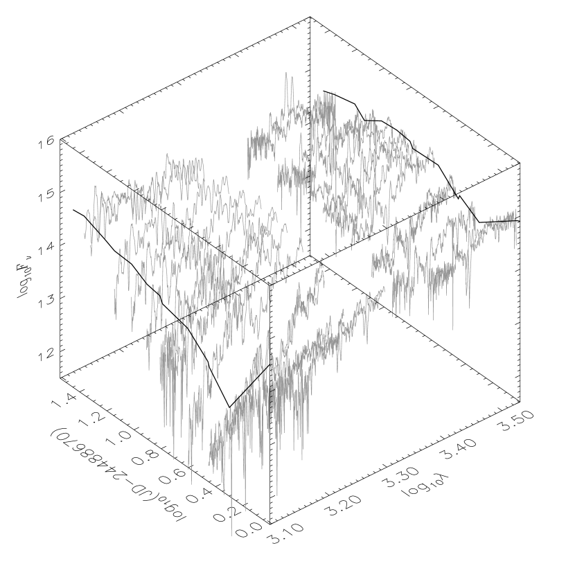
Figure 1: Time series of IUE SWP and LWP spectra at the fourteen phases of approximate simultaneity of the bands. The gap along the $\lambda$ axis occurs because the reduced SWP and LWP spectra are disjoint in wavelength. The mean wavelength integrated flux, $\bar{F}_{\lambda}$, for the SWP and LWP bands as a function of time (light curve) is plotted on the short wavelength and long wavelength walls of the plot cube, respectively.

Table 1 is a log of the observations that we have extracted from the IUE archive for both the low and high resolution spectrographs and for both the long and short wavelength cameras (LWP and SWP). Superscripts in Table 1 indicate approximately coincident pairs of SWP and LWP spectra. The spectra span a range of 144.75 days, from the initial fireball stage of the explosion, through the optically thick wind phase, to the nebular stage. Fig. 1 shows the fourteen pairs of approximately coincident SWP and LWP spectra as a function of time. We have discarded the portion of the SWP spectrum that lies below $\lambda 1250$ Å  due to the noisiness of the signal and contamination by geocoronal Lyman $\alpha$, and the portion of the LWP spectrum that lies below $\lambda 2400$ due to severe degradation of the signal. The gap in the $\lambda$ dimension arises because the reduced SWP and LWP spectra are disjoint in $\lambda$. The spectra have been recalibrated in wavelength and flux using the procedure of Massa and Fitzpatrick (1998), and de-reddened with a value of $E(B-V)=0.26$ (Chochol et al., 1997) using the galactic extinction curve of Fitzpatrick (1999).

We have calculated the light curves, $\bar{F}_{\rm SWP}(t)$ and $\bar{F}_{\rm LWP}(t)$, for the SWP and LWP bands by calculating the wavelength integrated mean flux, $\bar{F}_{\lambda}$, for each flux-corrected, de-reddened spectrum. The light curves are shown projected onto the sides of the data cube in Fig. 1. From the shape of the light curves and from the global shape of the spectra, we can see that the first two spectra were taken during a stage of rapid decline in UV flux and rapid softening of the UV spectral energy distribution, which is characteristic of the fireball stage of a nova. Later, the UV flux gradually increases and then becomes approximately constant and the spectral distribution gradually hardens as the nova progresses through the optically thick wind phase. Finally, the latest LWP spectrum in Fig. 1 shows prominent Mg II $hk$ emission, which indicates the onset of the optically thin nebular phase of the nova.

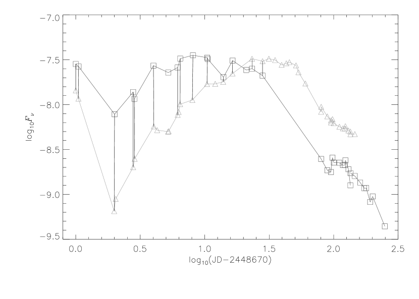
Figure 2: UV light curves. Mean $\lambda$ integrated flux, $\bar{F}_{\lambda}$, as a function of time for the LWP (squares, darker line) and SWP (triangles, lighter line). Vertical lines connecting the two light curves denote times of approximate simultaneity of the SWP and LWP observations where IUE colors were calculated (see text).

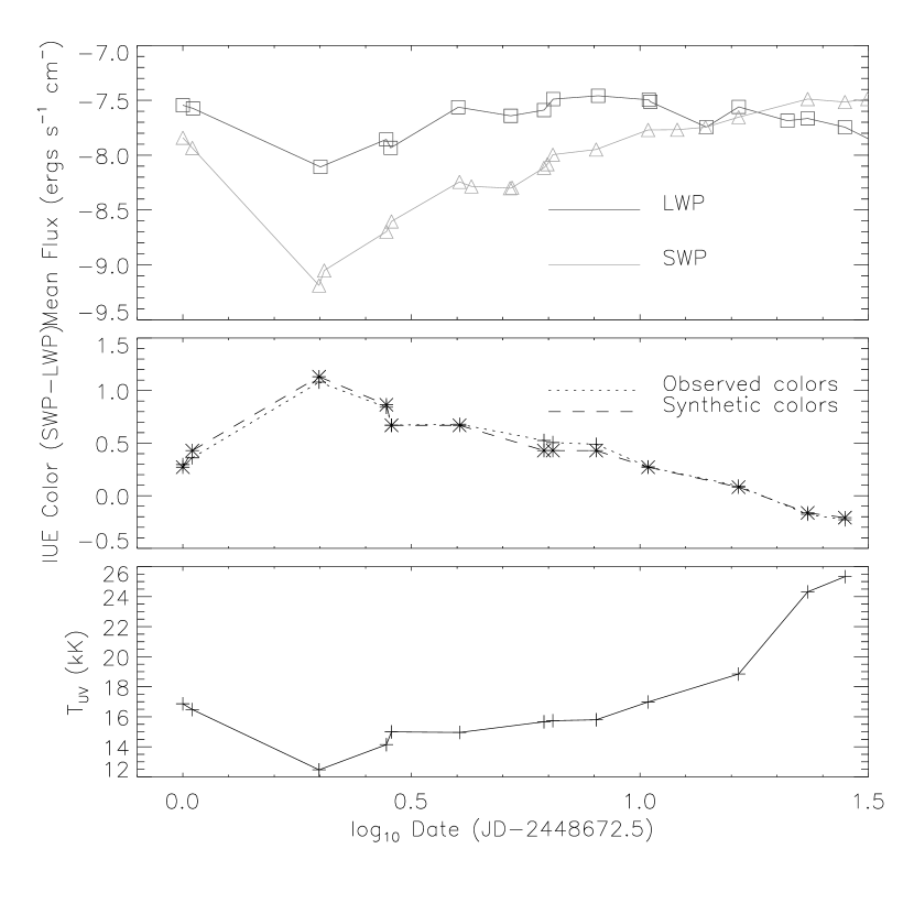
Figure 3: Deriving the time development of $T_{\rm UV}$ from the IUE data. Upper panel: Mean $\lambda$ integrated flux, $\bar{F}_{\lambda}$, for the LWP (squares, darker line) and SWP (triangles, lighter line). Center panel: IUE color, $\log\bar{F}_{\rm LWP}/\bar{F}_{\rm SWP}$. Observed (plus symbols, dotted line), synthetic (asterisks, dashed line). Lower panel: derived UV color temperature, $T_{\rm UV}$ (see text).

Fig. 2 shows the SWP and LWP light curves with the fourteen pairs of coincident spectra shown in Fig. 1 marked with vertical lines. The SWP light peaks about 20 days after the LWP light, which is consistent with the expected photometric time development of novae (see discussion is Section 3). We have formed the observed IUE color, $(SWP-LWP)_{\rm obs}$, at these times by computing the value of $\log(\bar{F}_{\rm LWP}/\bar{F}_{\rm SWP})$. The center panel of Fig. 3 shows the time development of $(SWP-LWP)_{\rm obs}$. As expected, the color becomes more positive (redder) during the fireball phase where $T_{\rm eff}$ is decreasing, and then gradually becomes more negative (bluer) during the optically thick wind phase where $T_{\rm eff}$ is increasing.

3 Modeling

We have calculated a set of atmospheric models that span a $T_{\rm eff}$ range of 12 to 30 kK in increments of 1 kK. The most important model parameters are the maximum expansion velocity of the linear velocity law, $v_{\rm o}$, which is $2000$ km s^-1 (Shore et al., 1994), the exponent of the exponential $\rho$ law, $N$, which is 3, the micro-turbulent velocity broadening width, $\xi$, which is $50$ km s^-1, and the abundances, $[\frac{A}{H}]$, which are solar. A linear velocity law and a value of $N$ equal to $3$ are consistent with a constant mass loss rate ($\dot{M}=$constant). The radius $R=r(\tau_{5000}=1)$, where $\tau_{5000}$ is the continuum optical depth at 5000Å, is adjusted for each value of $T_{\rm eff}$ to keep the bolometric luminosity, $L_{\rm bol}$, equal to $50\,000{\rm L}_{\odot}$. Pistinner et al. (1995) found that the calculated spectrum is relatively insensitive to the value of $L_{\rm bol}$, therefore, we do not vary this parameter. Abundance analyses of nova ejecta find them to have abundances of CNO and Fe that are enhanced with respect to the solar values (see, for example, Shore et al. (1997), or Hauschildt et al. (1994)). The enhanced metal abundance is thought to be caused by mixing of the ejected material with the metal rich White Dwarf (WD) material prior to the outburst, and by H burning during the thermonuclear runaway (TNR) that drives a nova explosion. Hauschildt et al. (1994) found $[\frac{CNO}{H}]\approx 1$ and $[\frac{Fe}{H}]\approx 0.3$, by number density with respect to the Sun. Therefore, we have also calculated a sub-set of the grid with the hydrogen abundance reduced to half of its solar value, by number, which makes $n_{\rm H}$ equal to $n_{\rm He}$ and $[\frac{A}{H}]$ equal to 0.3  (${{A/H}\over{{A/H_{\odot}}}}=2$ by number) for all metals.

Table 2 shows all the species that are treatable in NLTE with PHOENIX and indicates which ones have been included in the NLTE rate equations for each value of $T_{\rm eff}$ in the model grid. Because ionization stages that are important for some values of $T_{\rm eff}$ in the grid are unimportant for others, the species that are included in NLTE varies throughout the grid. In particular, the lowest ionization stages of some species that are included in the coolest models are excluded in hotter models, and higher ionization stages that are included in the hottest models are excluded in the cooler models. In practice, test calculations with the full suite of NLTE species were performed at a sparse sub-grid of models, and ionization stages that contribute less than $1\%$ of the total population of the species at all depths were treated in LTE for nearby models in the complete grid. Fig. 4 shows the synthetic spectra in the IUE wavelength range that were computed with the grid of models. The spectra were computed with a sampling, $\Delta\lambda$, of 0.03 Å  so that all spectral lines are well sampled, and then were degraded to the resolution of the IUE low resolution grating.

4 Analysis

The physical interpretation of the early photometric and spectroscopic time development of a nova in the UV is well summarized by Hauschildt et al. (1994). From Fig. 4 we see that as the $T_{\rm eff}$ of the model increases, the synthetic spectral energy distribution hardens. This is similar to the spectral hardening with time during the optically thick wind phase, and is opposite to the spectral softening with time during the fireball phase shown by the observed spectra in Fig. 1. During the brief fireball phase, an initial, thin shell of gas is ejected by the blast wave that is produced by the detonation. This initial fireball rapidly expands and cools adiabatically and becomes transparent after the first few days. This accounts for the initial rapid decline in UV brightness. Subsequently, we see the thicker, more extended secondary ejection that forms an expanding photosphere around the WD. During this optically thick wind phase, $T_{\rm eff}$ gradually increases as $\rho$ declines and the expanding atmosphere becomes increasingly less self-shielded from the central WD. At the same time, the declining $\rho$ also causes the photospheric radius ($r(\tau=1)$) to decrease so that deeper, hotter layers are progressively exposed. As a result, the peak of the emitted flux moves to progressively shorter $\lambda$, as can be seen from Fig. 2. During this stage the nova evolves at constant $L_{\rm bol}$ because the expanding atmosphere re-processes the energy emitted by the underlying WD, which is still burning H on its surface, and does not contain any energy sources of its own. The evolution of the UV spectrum during the optically thick wind phase can also be understood by considering the line blanketing. Near the beginning of the optically thick wind phase, the temperature of the atmosphere is such that Fe is mostly in the form of Fe I and  II, both of which have a very rich absorption spectrum in the UV. As a result, the UV flux is blocked by massive line absorption (the “iron curtain”). As the gas expands it thins and becomes increasingly radiatively heated by the central engine until it gradually takes on a more nebular character and Fe  becomes multiply ionized again. As a result, the UV opacity decreases and the UV flux increases and reaches a plateau about 50 days after the explosion. Some time after 150 days, the atmosphere expands to the point where the total optical depth through the atmosphere is less than unity and the continuum flux disappears.

4.1 Low resolution spectra

We have computed the synthetic IUE color, $(SWP-LWP)_{\rm syn}$, from the synthetic spectra using the same procedure that we used for $(SWP-LWP)_{\rm obs}$. Fig. 5 shows the relationship between $(SWP-LWP)_{\rm syn}$ and $T_{\rm eff}$. As expected, the color becomes bluer as $T_{\rm eff}$ increases. We note that throughout the $T_{\rm eff}$ range of our model grid, the slope of the $T_{\rm eff}(SWP-LWP)$ relation allows for an unambiguous $T_{\rm eff}$ determination from the $(SWP-LWP)$ color, given a sufficiently small error margin for the color.

We have assigned a Julian Date to each of the synthetic colors, $(SWP-LWP)_{\rm syn}$, shown in Fig. 5 by interpolation within the $(SWP-LWP)_{\rm obs}(t)$ relation. This allows us to arrange our models in a chronological sequence that reflects the time development of the nova. The center panel of Fig. 3 shows a comparison of the observed and synthetic color curves, $(SWP-LWP)_{\rm obs}(t)$ and $(SWP-LWP)_{\rm syn}(t)$. We have also assigned a time sequence of UV color temperatures, $T_{\rm UV}(t)$, to the sequence of observed colors, $(SWP-LWP)_{\rm obs}(t)$, by interpolation within the $T_{\rm eff}((SWP-LWP)_{\rm syn})$ relation. The lower panel of Fig. 3 shows the derived values of $T_{\rm UV}$ as a function of time. The UV radiation temperature in the IUE range initially cools from $\sim 17$ kK to $\sim 12$ kK during the fireball phase, then gradually heats up during the optically thick wind phase, till it reaches $\sim 24$ kK about 30 days after the explosion.

Because the IUE $\lambda$ range is close to the peak of the spectral energy distribution, $F_{\lambda}(\lambda)$, for this $T_{\rm eff}$ range, we have approximated the time development of $T_{\rm eff}$, $T_{\rm eff}(t)$, by setting it equal to $T_{\rm UV}(t)$. On this basis, we assign a synthetic spectrum from the model grid to each of the times marked in Fig. 2.

Fig. 6 shows the time development of four model quantities, according to the chronological ordering established above: $R(\tau_{5000}=1)$, $\log\rho(\tau_{5000}=1)$, the absolute value of the outward acceleration due to radiation pressure at a continuum optical depth of unity, $|a_{\rm rad}(\tau_{5000}=1)|$, and the total mass loss rate per year, $dM/dt$. As discussed above, the value of $R(\tau_{5000}=1)$ decreases throughout the optically thick wind phase because, although the atmosphere is expanding, the physical radius at which is becomes optically thick (the photosphere) is contracting as the gas becomes thinner. The recession of the photosphere to deeper atmospheric layers also causes the value of $\rho(\tau_{5000}=1)$ to increases during this time. The value of $|a_{\rm rad}(\tau_{5000}=1)|$ increases during this time because the radiation pressure increases as the atmosphere becomes hotter. For reference we have also plotted $g$, the inward acceleration due to gravity at $R(\tau_{5000}=1)$, assuming a $1.25M_{\odot}$ WD (Starrfield et al., 1997). The radiative acceleration of the atmosphere is discussed further below. The value of $g$ increases with time as $R(\tau_{5000}=1)$ decreases, but is always less that the value of $|a_{\rm rad}(\tau_{5000}=1)|$. At each time, the value of $dM/dt$ is independent of depth in the atmosphere, which is consistent with a linear velocity law, but not with a radiatively driven velocity law. The value of $dM/dt$ increases with time as the value of $|a_{\rm rad}|$ increases.

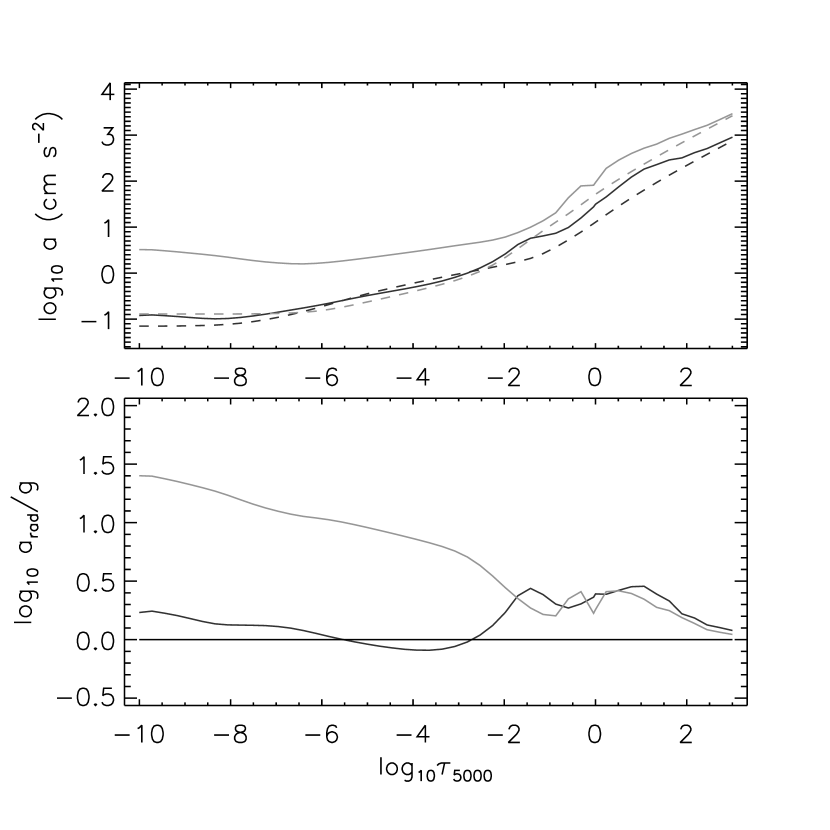
Figure 7: Comparison of $\log|a_{\rm rad}|$ and $\log g$ throughout two models that represent two different times during the optically thick wind phase. Darker line: JD 2448674.40320; lighter line: JD 2448688.85069. Upper panel: $\log|a_{\rm rad}|$ (solid line); $\log g$ (dashed line). Lower panel: $\log|a_{\rm rad}|/g$.

Fig. 7 shows a comparison of $\log|a_{\rm rad}|$ and $\log g$ as a function of depth throughout two of the models: 1) a model of $T_{\rm eff}=12$ kK, which corresponds to the time of the first spectrum of the optically thick wind phase (JD 2448674.40320), and 2) a model of $T_{\rm eff}=17$ kK, which corresponds to a time about two weeks later later (JD 2448688.85069). The figure also shows the difference of these quantities (ie $\log|a_{\rm rad}|/g$). For the cooler model, $|a_{\rm rad}|$ is greater than $g$ by as much as a factor of three at depths where $\log\tau_{\rm 5000}$ ranges from $2$ to $-2$. It is slightly less than $g$ in the $\log\tau_{\rm 5000}$ range between $-2.5$ and $-6$, and exceeds $g$ again in the outermost part of the atmosphere. The hotter model shows similar behavior in the $\log\tau_{\rm 5000}$ range between $2$ and $-2$, but $|a_{\rm rad}|$ remains greater than $g$ everywhere. These results suggest that radiation pressure could possibly play a role in determining the velocity structure of the wind. We are currently implementing the treatment of dynamics in PHOENIX with the goal of investigating this question further.

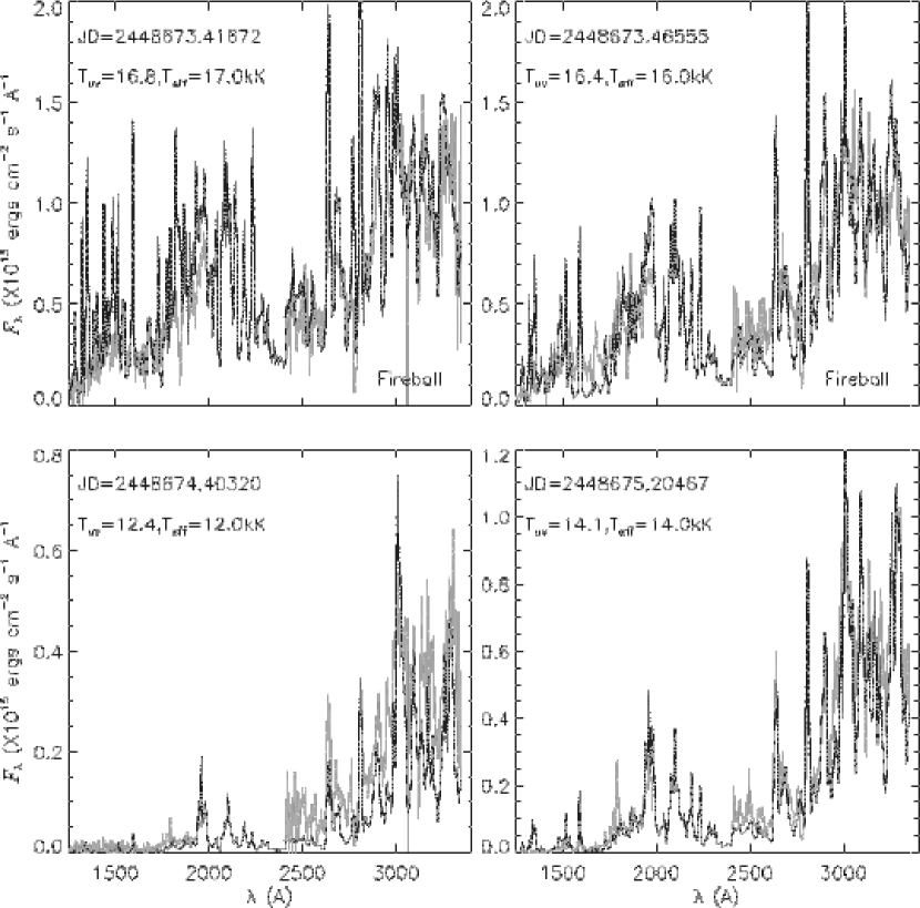
Figure 8: Comparison of observed (lighter line) and synthetic (darker line) spectra at the first twelve phases of approximate band simultaneity. The gap in $\lambda$ for the observed spectra occurs because the reduced SWP and LWP spectra are disjoint in $\lambda$. Each panel is labeled with the JD of the observed spectrum, the derived value of $T_{\rm UV}$ from the $(SWP-LWP)$ color, and the value of $T_{\rm eff}$ of the model used to synthesize the spectrum.

Figs. 8 through 10 show for each of these times the comparison between the observed spectrum and the synthetic spectrum for the model whose $T_{\rm eff}$ value is closest to the $T_{\rm UV}$ value of the observed spectrum. Because we do not know the angular diameter of Cygni 92, we arbitrarily adjust the flux level of the observed spectra to approximately match the absolute flux level of the synthetic spectra. However, note that in keeping with the condition of constant $L_{\rm bol}$, the same scale factor has been used in all plots (ie. individual pairs of observed and synthetic spectra have not had their flux calibration “tuned”). The observed spectrum in each panel has a gap in the middle because the reduced SWP and LWP spectra are disjoint in $\lambda$. For times later than JD 2448683, the Mg II $hk$ resonance doublet at $\lambda 2800$ becomes increasingly strong in emission with respect to the pseudo-continuum, which indicates that the nova is becoming increasingly nebular at that time.

For the fireball phase, and for all times throughout the optically thick wind phase up to JD 2448682.8368, a synthetic spectrum of $T_{\rm eff}\approx T_{\rm UV}$ provides a good fit to the global shape of the pseudo-continuum throughout the entire IUE $\lambda$ range. This is significant because we see from both Figs. 1 and 4 that the SWP range is sensitive to $T_{\rm eff}$ in this $T_{\rm eff}$ range.

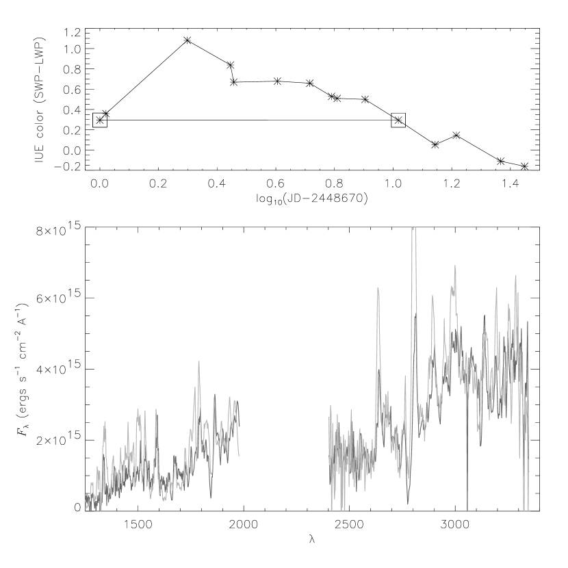
Figure 12: Comparison of fireball and optically thick wind phase at equal color. Upper panel: observed IUE color $(SWP-LWP)$ as a function of time. The squares connected by the horizontal line indicate the two phases being compared in the lower panel. Lower panel: Comparison of fireball spectrum (darker line) and optically thick wind phase spectrum (lighter line) at the two phases indicated in the upper panel.

To illustrate the similarity of the fireball phase to the optically thick wind phase, we have identified two times, JD2448673.4167 (fireball phase), and JD2448686.3241 (optically thick wind phase) at which the $(SWP-LWP)_{\rm obs}$ color, and, therefore, the value of $T_{\rm UV}$, is approximately the same. Fig. 12 shows a comparison of the IUE spectra at these two times. Both spectra have been multiplied by the same factor to approximately remove the dilution factor, but they have not been shifted with respect to one another. The absolute flux level and overall shape of the pseudo-continuum is approximately the same. However, the optically thick wind phase spectrum exhibits significantly stronger emission lines than the fireball phase spectrum. The difference in the strength of the emission lines is due to the greater amount of Doppler broadening from a steeper velocity gradient through the LFR in the thin fireball (Hauschildt et al., 1994).

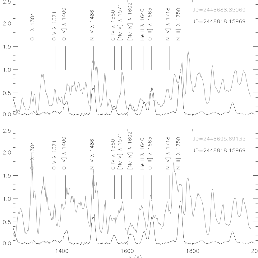
Figure 11: The last two observed spectra that were fit in Fig. 10 (JD2448688.85069 and JD2448695.69135) (lighter line). A spectrum from the nebular phase of the outburst taken over 100 days later (darker line). The line annotations refer to nebular lines.

For the last two times shown, JD2448688.8507 and JD2448695.6914, none of the synthetic spectra provide as close a fit as that for earlier times. Furthermore, in contrast to what we find for earlier times, the closest fit synthetic spectrum is that of a model for which $T_{\rm eff}$ is significantly lower that the observed value of $T_{\rm UV}$. Fig. 11 shows the observed spectrum at these two times compared with an IUE low resolution spectrum that was taken over 100 days later (SWP45135). At the later time, the nova has become nebular and exhibits a pure emission spectrum with permitted, semi-forbidden, and forbidden lines in the UV. The velocity of the outflowing gas during the nebular phase is $4500$ km s^-1 ((Shore et al., 1997)). Therefore, we have shifted the nebular spectrum red-ward by $2000$ km s^-1. The nebular emission lines labeled in Fig. 11 were identified using Table 1 in Shore et al. (1997). The comparison of the nebular phase spectrum with the two earlier spectra shows that by JD2448688.8507 many of the nebular lines were already present in the spectrum. The expanding atmosphere was already partially nebular by JD2448688.8507 in that many of the nebular lines had already begun to “contaminate” the optically thick wind phase spectrum. As a result, we expect that PHOENIX models will provide an increasingly worse fit beyond this time because PHOENIX is capable of modeling only the component of the outburst that constitutes an optically thick atmosphere.

4.2 High resolution spectra

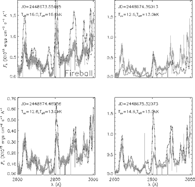
Figure 13: Comparison of high resolution observed (lighter line) and synthetic (darker line) spectra at eight phases. Each panel is labeled with the JD of the observed spectrum, the interpolated value of $T_{\rm UV}$ from the time vs $(SWP-LWP)$ relation (see text), and the value of $T_{\rm eff}$ of the model used to synthesize the spectrum. Upper left panel: the dashed line is the synthetic spectrum of a supernova model with $T_{\rm eff}$ equal to 12 kK.

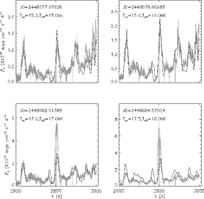
Figure 14: See Fig. 13

Figs. 13 and 14 show a time sequence of high resolution IUE spectra in the LWP pass band that overlaps in time the sequence shown in Figs. 8 through 10. Synthetic spectra have been assigned to each time by interpolation in the time vs $T_{\rm UV}$ relation that was derived from the low resolution spectra (lower panel of 3). The prominent emission feature at $\lambda 2800$ is the $hk$ resonance doublet of Mg II. The Mg II $hk$ lines become stronger with time because the expanding atmosphere gradually becomes more nebular. As a result, the models, which only account for the photospheric part of the expanding gas shell, increasingly underpredict the strength of these lines as time increases. The prominent emission features at $\lambda 2630$ and $\lambda 2900$, which are approximately reproduced by the models at many times, are not emission lines, but are regions of relatively lower line opacity through which more flux escapes than through the neighboring regions.

Generally, the models approximately reproduce the broad features of the high resolution spectra during the optically thick wind phase. However, there are discrepancies in the detailed fit. One possible source of discrepancy is the distribution of metal abundances. The nova ejecta may be depleted in H and enriched in C, N, and O as a result of WD material having been mixed into the accreted layers, or as a result of nuclear processed elements from the surface H burning that drives the nova explosion having been ejected. Hauschildt et al. (1994) found that $[\frac{CNO}{H}]$ is approximately one while $[\frac{Fe}{H}]$ is only about 0.3. Some discrepancy may also be due to the form of the velocity law. If the ejecta are being driven outward by radiation pressure at this stage, then $v(r)$ may have the power law form of a wind rather than a linear form (Castor et al., 1975). Indeed, since the time of McLaughlin (1947) it has been observed that relatively blue shifted spectral absorption components arise in relatively deep layers of the expanding atmosphere, which suggests a more complex velocity law than the linear one employed here. We are currently in the process of converging power law wind models. Another possible source of discrepancy is inhomogeneities in the expanding gas shell, which have been observed (see, for example, Payne-Gaposchkin (1957) or Shore et al. (1997)), and which are expected to arise if the velocity field is complex. These will serve to make the line profiles more complex than those predicted with a homogeneous model.

The upper left panel in Fig. 13 shows the fit to the only high resolution spectrum taken during the fireball phase. At this resolution it is clear that the nova models systematically over-predict the strength of all emission features by a factor of approximately two. The dashed line is the synthetic spectrum of a model with $T_{\rm eff}$ equal to $12000$ K, $v_{\rm max}$ equal to $4000$ km s^-1, and $N=7$ rather than $3$ ($\rho(r)~{}\alpha~{}r^{-N}$). This model is much thinner in the radial direction and has much steeper $\rho(r)$ and $v(r)$ gradients than the models in our nova grid. Moreover, because $N>3$, the motion of the atmosphere does not correspond to a constant mass loss rate, but, rather to homologous expansion. The characteristics of this model are more similar to those of supernova models rather than typical nova models. Such a model yields a synthetic spectrum with much weaker emission features than that of a more typical nova model because the steeper $v(r)$ gradient leads to a greater Doppler smearing of the emergent spectrum. As a result, this model provides a significantly better fit to the observed spectrum. This is consistent with the idea that the fireball phase is due to a thin shell of gas that is ejected by the blast wave before the expanding atmosphere that causes the optically thick wind phase develops. We note that the best fit value of $T_{\rm eff}$ for the fireball spectrum is $4000$ K lower when it is fit with the thinner, steeper model rather than a typical nova model. Hauschildt et al. (1994) found that a thin shell model with a steep ($N=15$) $\rho$ law and enhanced CNO  and Fe  abundances was required to fit the first two observed spectra. A comparison of the 2600 to 3000 Å  region in their Fig. 5b with Fig. 13 shows that we achieve a better fit to the fireball phase with a solar abundance model than they did. The improvement may be due to the greater number of species treated in NLTE.

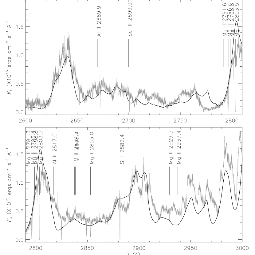
Figure 15: Comparison of high resolution observed (lighter line) and synthetic (darker line) spectra at a representative time during the optically thick wind phase. The strongest lines in the spectrum synthesis, other than Fe group lines, have been labeled with their identifications.

Fig. 15 shows a representative high resolution observed spectrum from the early optically thick wind phase (LWP22457, JD2448677.67626, $T_{\rm UV}\approx 15$ kK). Also shown is the best fit synthetic spectrum. The plot has been labeled with the identifications of the strongest lines, as determined by the spectrum synthesis calculation. During the line identification procedure the Fe group elements were ignored to prevent the plot from being completely saturated with the labels of Fe II and, to a lesser extent, of Fe I, Fe III, Ti II, Cr II, Co II, and Ni II, which are the most important source of opacity at most wavelength points.

4.3 Abundance effects

Fig. 16 shows a comparison between the synthetic spectra of models with solar abundance and those that are hydrogen deficient in a representative region of the IUE spectral range. Reducing $n_{\rm H}$ to half of its solar value by number makes $\frac{n_{\rm He}}{n_{\rm H}}=1$, and $[\frac{A}{H}]=0.3~{}({{A/H}\over{{A/H}_{\odot}}}=2$ by number) for all metals. From Fig. 16 we see that the hydrogen deficiency suppresses the overall flux throughout the near UV by approximately a factor of two while preserving the relative strength of the spectral features. We also show for comparison the synthetic spectrum of a hydrogen deficient model with a value of $T_{\rm eff}$ that is 1kK greater than that of the solar abundance model. The synthetic spectrum from the hydrogen deficient model with the larger $T_{\rm eff}$ approximately matches both the overall flux level and the detailed structure of the synthetic spectrum of the solar abundance model throughout the IUE wavelength range. To a first approximation, a solar abundance model is interchangeable with a hydrogen deficient model that is 1 kK hotter when fitting the near UV spectrum. For the accuracy of the fitting done here, it is necessary to fit models to a region of the spectrum other than the UV to disentangle $T_{\rm eff}$ from $[\frac{A}{H}]$.

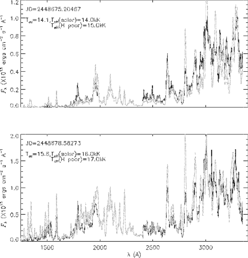
Figure 17: Comparison of observed (darker line) and synthetic (lighter lines) spectra at two representative times. Lighter solid line: $[{A\over H}]=0$ (solar abundance) models; lighter dashed line: $[{A\over H}]=0.3$ models.

Fig. 17 shows a comparison of the observed spectrum and synthetic spectra from the best fit solar abundance model ($T_{\rm eff}=T_{\rm UV}$) and a hydrogen deficient model of $T_{\rm eff}=T_{\rm UV}+1$ kK at two times during the optically thick wind phase. From a visual inspection, both synthetic spectra provide approximately the same goodness of fit at both times. We conclude that the result of fitting hydrogen deficient models to the observed spectral sequence is to shift the derived $T_{\rm eff}$ evolution upward by approximately 1 kK. There are no spectral features in this range that distinguish between two such models. Therefore, there is a degeneracy in $T_{\rm eff}$ and $n_{\rm H}$, at least within the range of parameters explored here. Superficially, the degeneracy arises because a larger value of $T_{\rm eff}$ enhances the UV flux (see Fig. 4), whereas the increased value of $[{Fe\over H}]$ suppresses the UV flux. The net result is that increasing both in a particular proportion will lead to an approximately similar UV flux spectrum. A more fundamental discussion of spectral similarity and non-uniqueness problems in atmospheric models of novae can be found in Pistinner and Shaviv (1996).

5 Conclusion

We conclude that the UV radiation temperature ($T_{\rm UV}$) is a good measure of $T_{\rm eff}$ during the early stage of the nova when the spectrum is purely that of an optically thick wind. We find that this stage lasts until JD2448682.8368, which is about 10 days after the first fireball phase spectrum was taken. During this interval, PHOENIX models are able to reproduce the overall shape of the low resolution UV spectra in the IUE range. This is significant because the nova photosphere increases in $T_{\rm eff}$ by $\approx 5000$ K during this time, and the hardness of the near UV radiation field is sensitive to $T_{\rm eff}$ in the range from ten to twenty kK. The models provide a moderately good fit to the high resolution spectra during the optically thick wind phase, but there are significant discrepancies which are due to, among other things, a non-solar abundance distribution due to nuclear processing, an inaccurate velocity law, and inhomogeneities in the expanding atmosphere.

Models in which H is depleted to a tenth of its solar value and in which $\frac{A}{H}$ is twice the solar value provide a similarly good fit to the observed spectra in the UV if the value of $T_{\rm eff}$ of the model is increased by $\approx 1$ kK. We conclude that $[\frac{A}{H}]$ and $T_{\rm eff}$ are degenerate parameters when fitting models to the near UV spectrum. It is necessary to fit models to another $\lambda$ region to uniquely determine $T_{\rm eff}$ and $[\frac{A}{H}]$.

The high resolution spectrum of the fireball phase of the nova has weaker emission features than an optically thick wind phase spectrum of the same best fit $T_{\rm eff}$. The fireball phase spectrum is better fit by a supernova model, in which the atmosphere is thinner and has a steeper $\rho(r)$ and $v(r)$ gradient.

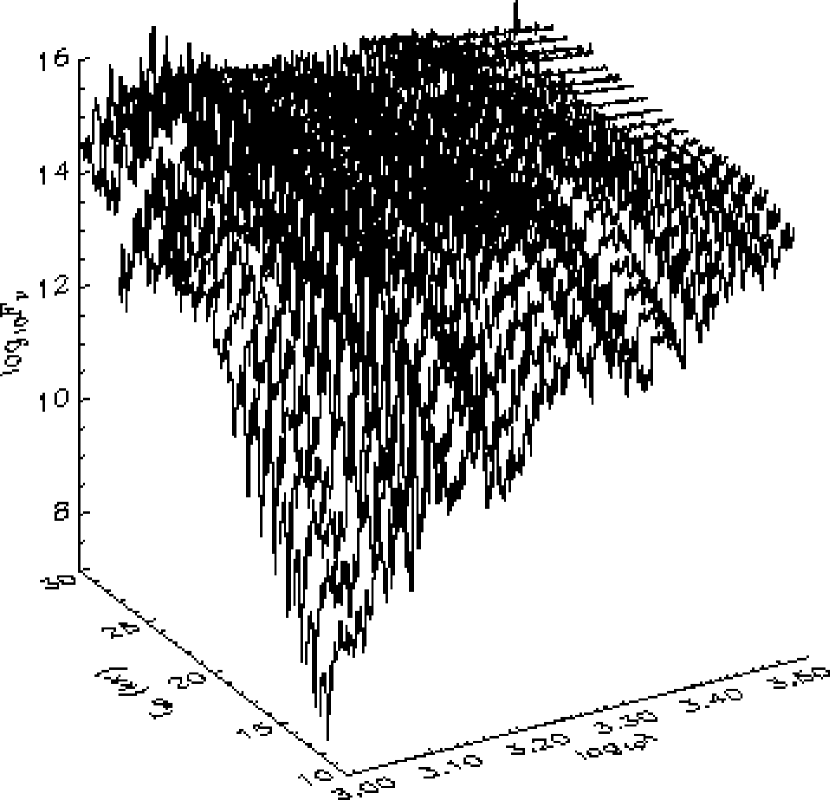
Figure 4: Model flux surface for nova grid consists of closely spaced synthetic spectra. Surface gives general overview of how the global flux level and spectral energy distribution changes with $T_{\rm eff}$.

Figure 5: Model $T_{\rm eff}$ as a function of synthetic color $(SWP-LWP)$.

Figure 6: The time development of four model quantities according to the chronological ordering based on the IUE color (see text). Upper left panel: $R(\tau_{\rm 5000}=1)$; upper right panel: $\log\rho(\tau_{\rm 5000}=1)$; lower left panel: $|a_{\rm rad}(\tau_{\rm 5000}=1)|$, and, for reference, the value of $g$ assuming a 1.25 $M_{\odot}$ WD; lower right panel: $dM/dt$.

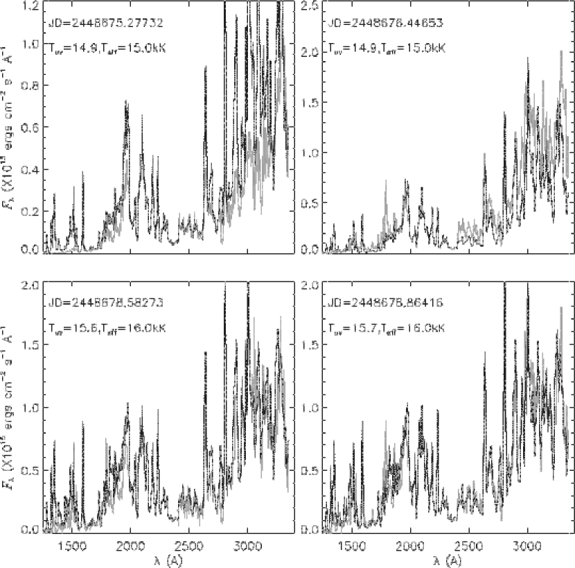
Figure 9: See Fig. 8

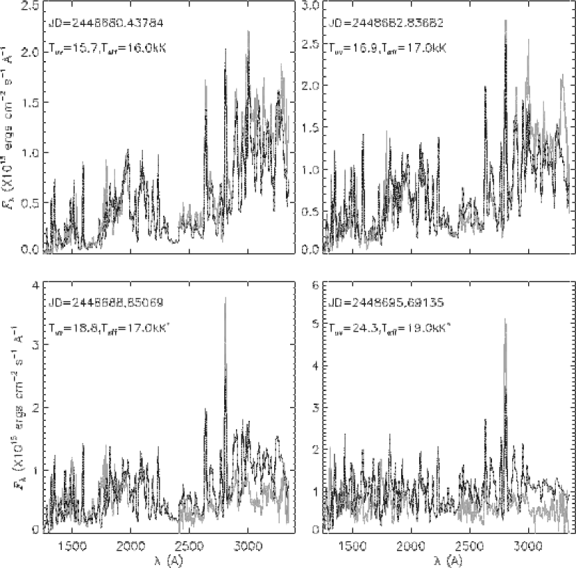
Figure 10: See Fig. 8

Figure 16: Comparison of synthetic spectra with various values of $T_{\rm eff}$ and $[\frac{A}{H}]$. Lighter line: Solar abundances, $T_{\rm eff}=14$ kK (upper panel) and $16$ kK (lower panel). Darker solid line: $[\frac{A}{H}]=0.3$, $T_{\rm eff}=14$ kK (upper panel) and $16$ kK (lower panel). Darker dashed line: $[\frac{A}{H}]=0.3$, $T_{\rm eff}=15$ kK (upper panel) and $17$ kK (lower panel).

Table 1: Log of low resolution IUE spectra

LWP		SWP
Exp. No.	JD-2448000	Exp. No.	JD-2448000
${\rm lwp}22425^{1}$	673.40	${\rm swp}44030^{1}$	673.41
${\rm lwp}22426^{2}$	673.45	${\rm swp}44031^{2}$	673.46
${\rm lwp}22430^{3}$	674.40	${\rm swp}44039^{3}$	674.40
${\rm lwp}22434^{4}$	675.19	${\rm swp}44040$	674.45
${\rm lwp}22435^{5}$	675.25	${\rm swp}44043^{4}$	675.20
${\rm lwp}22448$	676.41	${\rm swp}44044^{5}$	675.27
${\rm lwp}22449^{6}$	676.45	${\rm swp}44050^{6}$	676.44
${\rm lwp}22456^{7}$	677.62	${\rm swp}44051$	676.69
${\rm lwp}22459^{8}$	678.57	${\rm swp}44055^{7}$	677.61
${\rm lwp}22462^{9}$	678.86	${\rm swp}44056$	677.66
${\rm lwp}22470$	680.50	${\rm swp}44060^{8}$	678.58
${\rm lwp}22483^{10}$	682.86	${\rm swp}44062$	678.69
${\rm lwp}22485$	682.94	${\rm swp}44064^{9}$	678.86
${\rm lwp}22513^{11}$	686.38	${\rm swp}44073$	680.43
${\rm lwp}22533^{12}$	688.85	${\rm swp}44086^{10}$	682.83
${\rm lwp}22573$	693.43	${\rm swp}44102$	684.48
${\rm lwp}22592^{13}$	695.68	${\rm swp}44115^{11}$	686.32
${\rm lwp}22635^{14}$	700.49	${\rm swp}44130^{12}$	688.85
${\rm lwp}23077$	752.34	${\rm swp}44174^{13}$	695.69
${\rm lwp}23134$	761.76	${\rm swp}44193^{14}$	700.49
${\rm lwp}23170$	767.66	${\rm swp}44209$	703.85
${\rm lwp}23188$	770.31	${\rm swp}44233$	707.50
${\rm lwp}23210$	772.64	${\rm swp}44268$	711.89
${\rm lwp}23276$	783.24	${\rm swp}44305$	715.32
${\rm lwp}23312$	790.26	${\rm swp}44338$	717.77
${\rm lwp}23348$	794.42	${\rm swp}44377$	723.43
${\rm lwp}23351$	795.67	${\rm swp}44389$	725.76
${\rm lwp}23399$	802.58	${\rm swp}44439$	732.75
${\rm lwp}23424$	807.15	${\rm swp}44632$	752.31
${\rm lwp}23425$	807.20	${\rm swp}44634$	752.42
${\rm lwp}23426$	807.31	${\rm swp}44717$	761.70
${\rm lwp}23501$	818.17	${\rm swp}44761$	767.67
${\rm lwp}23599$	833.04	${\rm swp}44762$	767.70
${\rm lwp}23670$	845.01	${\rm swp}44790$	770.31
${\rm lwp}23706$	851.43	${\rm swp}44808$	772.64
${\rm lwp}23802$	864.30	${\rm swp}44901$	783.26
${\rm lwp}23869$	873.00	${\rm swp}44937$	790.24
${\rm lwp}24153$	921.60	${\rm swp}44970$	794.43

Note. — Matching superscripts indicate approximately simultaneous LWP/SWP pairs.

Table 2: Ranges of $T_{\rm eff}$ (in kK) in the model grid for which each ionization stage of each element was treated in NLTE.

Element	Ionization Stage
	I	II	III	IV	V	VI	VII
H	All	$\cdots$	$\cdots$	$\cdots$	$\cdots$	$\cdots$	$\cdots$
He	All	All	$\cdots$	$\cdots$	$\cdots$	$\cdots$	$\cdots$
Li	None	None	$\cdots$	$\cdots$	$\cdots$	$\cdots$	$\cdots$
C	12-24	All	All	All	$\cdots$	$\cdots$	$\cdots$
N	All	All	All	All	None	None	$\cdots$
O	All	All	All	All	None	None	$\cdots$
Ne	All	$\cdots$	$\cdots$	$\cdots$	$\cdots$	$\cdots$	$\cdots$
Na	12-24	All	All	All	None	None	$\cdots$
Mg	12-24	All	All	All	None	None	$\cdots$
Al	12-24	All	All	All	None	None	$\cdots$
Si	12-24	All	All	All	30	None	$\cdots$
P	12-22	12-22	12-22	12-22	None	None	$\cdots$
S	12-24	All	All	All	30	None	$\cdots$
K	None	None	None	None	None	$\cdots$	$\cdots$
Ca	12-24	12-24	All	All	All	None	None
Ti	None	None	$\cdots$	$\cdots$	$\cdots$	$\cdots$	$\cdots$
Fe	12-24	All	All	All	All	None	$\cdots$
Co	None	None	None	$\cdots$	$\cdots$	$\cdots$	$\cdots$
Ni	None	25-30	25-30	25-30	30	None	$\cdots$

Note. — Elements in bold face have been added since the last NLTE PHOENIX analysis of Cygni 1992. Those in italics have had their treatment improved since the last analysis.

References

- Castor et al. (1975) Castor, J.D., Abbott, D., & Klein, R., 1975, ApJ, 195, 157
- Chochol et al. (1997) Chochol, D., Grygar, J., Pribullai, T., Komzik, R., Hric, L., & Elkin, V. 1997, A&A, 318, 908
- Collins (1992) Collins, M., 1992, IAU Circ. No. 5454
- Fitzpatrick (1999) Fitzpatrick, E. 1999, PASP, 111, 63
- Hauschildt & Baron (1999) Hauschildt, P. H. & Baron, E., 1999, J. Comput. App. Math. 102, 41
- Hauschildt et al. (1994) Hauschildt, P. H., Starrfield, S., Austin, S., Wagner, R. M., Shore, S. N., & Sonneborn, G., 1994, ApJ, 422, 831
- Massa and Fitzpatrick (1998) Massa, D. & Fitzpatrick, E. 1998, A&A, 193, 1122
- McLaughlin (1947) McLaughlin, D., 1947, PASP, 59, 244
- Payne-Gaposchkin (1957) Payne-Gaposchkin, C., 1957, The Galactic Novae (Amsterdam: North-Holland)
- Pistinner and Shaviv (1996) Pistinner, S. & Shaviv, G., 1996, ApJ, 461, L45
- Pistinner et al. (1995) Pistinner, S., Shaviv, G., Hauschildt, P. & Starrfield, S., 1995, ApJ451, 724
- Shore et al. (1994) Shore, S. N., Sonneborn, G., Starrfield, S., Gonzalez-Riestra & R., Polidan, R. S., 1994, ApJ, 421, 344
- Shore et al. (1997) Shore, S. N., Starrfield, S., Ake, T. B. & Hauschildt, P. H., 1997, ApJ, 490, 393
- Short et al. (1999) Short, C. I., Hauschildt, P. H., & Baron, E., 1999, ApJ, 525, 375
- Starrfield et al. (1997) Starrfield, S., Truran, J. W., Wiescher, M. C., & Sparks, W. M., 1997, MNRAS, 296, 502