Emission from Bow Shocks of Beamed Gamma-Ray Bursts

Abstract

Beamed $\gamma$-ray burst (GRB) sources produce a bow shock in their gaseous environment. The emitted flux from this bow shock may dominate over the direct emission from the jet for lines of sight which are outside the angular radius of the jet emission, $\Theta_{b}$. The event rate for these lines of sight is increased by a factor of $\sim 260(\Theta_{b}/5^{\circ})^{-2}$. For typical GRB parameters, we find that the bow shock emission from a jet of half-angle $\sim 5^{\circ}$ is visible out to tens of Mpc in the radio and hundreds of Mpc in the X-rays. If GRBs are linked to supernovae, studies of peculiar supernovae in the local universe should reveal this non-thermal bow shock emission for weeks to months following the explosion.

1 INTRODUCTION

The afterglows of Gamma-ray bursts (GRBs) are most naturally described by the so-called “fireball” model (see e.g., Paczyński & Rhoads 1993; Katz 1994; Mészáros & Rees 1993, 1997; Waxman 1997a,b; Sari, Piran, & Narayan 1998). In this model, a compact source releases a large amount of energy over a short time and produces a relativistically expanding fireball. Eventually the fireball interacts with the circumburst medium, producing a spherical relativistic shock in it. As the shock decelerates due to the accumulation of mass from the external medium, it approaches a self-similar solution (Blandford & McKee 1976) and produces delayed synchrotron emission in X-rays, optical and radio, similar to the observed afterglows. The model generically yields power-law spectra and lightcurves in general agreement with observations at X-ray (Costa et al. 1997), optical (van Paradijs et al. 1997) and radio (Frail et al. 1997) wavelengths. Precise positions have allowed redshifts to be measured for a number of GRBs (Metzger et al. 1997), providing a definitive proof of their cosmological origin.

Recent observational evidence indicates that at least some GRB are not spherical explosions. A broad-band break in the lightcurve power-law index was predicted for shocks produced by collimated jets due to the lateral expansion of the jet when its Lorentz factor drops below the inverse of its opening angle (Rhoads 1997, 1999a,b; Panaitescu & Mészáros 1999). Such breaks have been seen in GRB 990510 (Stanek et al. 1999; Harrison et al. 1999), GRB 991216 (Halpern et al. 2000), and GRB 000301C (Sagar et al. 2000; Masetti et al. 2000; Jensen et al. 2000; Berger et al. 2000). The ratio of the spectral index to the light curve index also suggests non-spherical energy ejection for some events (e.g. GRB 991216: Garnavich et al. 2000).

The possibility that GRBs are associated with a rare sub-class of supernovae (SNe) was advocated recently based on a possible SN component in the lightcurves of GRB 980326 (Bloom et al. 1999) and GRB 970228 (Reichart 1999) and the association of SN1998bw with GRB 980425 (Galama et al. 1999; Kulkarni et al. 2000). In this case the GRB emission needs to be beamed in order to achieve the high Lorentz factor required for GRB outflows, despite the massive progenitor envelope and the low energy yield of SNe (MacFadyen, Woosley, & Heger 1999; Khokhlov at al. 1999; Umeda 2000).

The current state of knowledge leaves two major questions open: (i) are GRBs associated with rare SNe?; and (ii) if so, what is the characteristic collimation angle of the energy release? The collimation angle has important implications on the nature of the central engine. If the average angular radius of the two opposing jets in collimated GRBs is $\Theta_{b}$, then the total energy release will be reduced by a factor $2\pi\Theta_{b}^{2}/4\pi=\Theta_{b}^{2}/2$ and the event rate will be increased by the inverse of this factor. In this paper we propose a direct observational probe that will help answer these questions.

When a transient relativistic jet (equivalent to a relativistic “bullet”) moves into the circumburst medium (be it the interstellar medium or a progenitor wind), a bow shock is generated in front of the jet. The bow shock accelerates electrons which emit synchrotron radiation, similarly to the primary shock in front of the jet. For observers situated within the cone of the jet emission, the bow shock emission will be sub-dominant relative to the jet emission due to relativistic motion of the jet towards the observer. However, for highly collimated outflows, most lines of sight lie outside the jet cone, and for those – the bow shock emission may dominate. In particular, if GRBs originate in SNe then the bow shock emission will add a strong non-thermal component to the emission from the SN remnants extending from the radio to the X-ray bands. This emission will extend over much longer times compared to the jet emission since the Lorentz factor of the bow shock is typically much smaller than that of the jet, resulting in a smaller relativistic compression of time in the observer’s frame. In the following sections we will apply the same model used ordinarily for the primary fireball shock, to calculate the flux in this non-thermal bow-shock component. In §2 we present our model for the bow shock emission; in §3 we show our numerical results; and finally, in §4, we summarize our main conclusions.

2 MODEL

The impulsive ejection of a relativistic jet from the GRB source results in a thin disk of material moving outwards and expanding, which we refer to as a relativistic bullet. As long as the angular radius of the bullet relative to the center of the explosion, $\Theta_{b}$, is much larger than the inverse of its Lorentz factor, the bullet will expand as if it is part of a spherically symmetric fireball. This follows from the relativistic transformation of velocities, which implies that the propagation speed of a signal in the perpendicular direction to the bullet motion cannot exceed $\sim c/\gamma_{b}$ in the frame of the stationary ambient medium. For simplicity, we limit our discussion to this regime.

In our model we assume that as the relativistic bullet moves through the ambient medium, it deposits a fraction of its kinetic energy in each infinitesimal distance it travels. We treat this energy deposition as a sequence of point explosions, which drive shocks into the surrounding medium. The combination of this sequence of small shocks results in a conical bow shock structure behind the bullet.

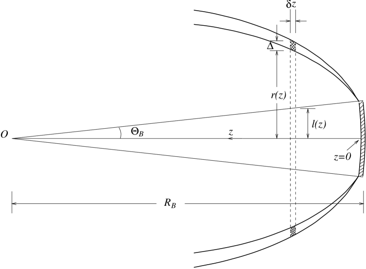
Figure 1: Geometry of the bow shock.

Figure 1 illustrates the geometry of the bow shock. We use cylindrical coordinates, with the $z$-axis connecting the bullet center to the source. The distance between the source and the bullet is denoted as $R_{b}$. We assume that observers are located perpendicular to the $z$-axis, with $\theta=0$ along the source-observer axis. Next we consider a slice of the bow shock geometry perpendicular to the $z$-axis. The slice is a cylindrical shell of height $\delta z$, thickness $\Delta$ and inner radius $r$. As the bullet passes through a point $z$ it has a radius $l(z)$ and a Lorentz factor $\gamma_{b}(z)$. The amount of thermal energy $\delta E$ which gets deposited by the bullet in the surrounding medium as it moves an extra distance $\delta z$, is then given by

$$\delta E=(\gamma_{b}-1)\pi l^{2}\ \delta z\ n\mu_{e}m_{p}c^{2},$$ (1)

where $n$ is the electron number density of the external medium, and $\mu_{e}m_{p}$ is the ion mass per electron. We assume that a fraction $\varepsilon$ of the energy stored in the “causally-connected” edge of the bullet is transferred to the external medium. The “causally-connected” edge of the bullet is defined to be the region occupying an angular size $1/\gamma_{b}$ from the bullet edge. The energy deposited in the infinitesimal distance interval $\delta z$ drives a shock into the ambient gas. The gas behind the shock is piled into an outgoing thin shell. The shock expands perpendicular to the $z$-axis, but due to the time delay between the energy deposition at different points along the $z$-axis, the sum of the fronts generated by these points defines a conical shape for the resulting bow shock. We denote the Lorentz factor of the outgoing shell in the frame of the unshocked gas by $\gamma$ . The electron number density $n^{\prime}$ and internal energy density $e^{\prime}$ of the shocked gas in the frame comoving with the shell can be written as (Blandford & McKee 1976)

$$n^{\prime}=\frac{\hat{\gamma}\gamma+1}{\hat{\gamma}-1}n,$$ (2)

$$e^{\prime}=\frac{\hat{\gamma}\gamma+1}{\hat{\gamma}-1}(\gamma-1)n\mu_{e}m_{p}c^{2},$$ (3)

where $\hat{\gamma}$ is the adiabatic index of the shocked gas which changes from $4/3$ and $5/3$ as the shock velocity changes from the relativistic to the non-relativistic regime. We interpolate between these regimes using the simplified expression $\hat{\gamma}\approx(4\gamma+1)/(3\gamma)$ (Dai, Huang & Lu 1999). Equations (2) and (3) then become

$$n^{\prime}=4\gamma n,$$ (4)

$$e^{\prime}=4b\gamma^{2}n\mu_{e}m_{p}c^{2},$$ (5)

where $b=(\gamma-1)/\gamma$. Note that equations (4) and (5) are appropriate for both the relativistic and non-relativistic regimes. The total kinetic energy of the shell is

$$E_{k}=\pi(r^{2}-l^{2})\ \delta z\ n\mu_{e}m_{p}c^{2}\beta^{2}\gamma^{2},$$ (6)

where $\beta^{2}=1-1/\gamma^{2}$. Conservation of energy implies, $E_{k}=\varepsilon\xi\delta E$, where

$$\xi=\frac{2\Theta_{b}\gamma_{b}-1}{\Theta_{b}^{2}\gamma_{b}^{2}}\ \ \ \ {\rm for}\ \gamma_{b}\geq\frac{1}{\Theta_{b}}$$ (7)

is the ratio between the volumes of the causaly-connected region near the edge of the bullet (with angular size $1/\gamma_{b}$) and the entire volume of the bullet. We therefore obtain

$$\gamma=\sqrt{1+\varepsilon\xi(\gamma_{b}-1)\frac{l^{2}}{r^{2}-l^{2}}}=\sqrt{1+f\frac{l^{2}}{r^{2}-l^{2}}},$$ (8)

where $f=\varepsilon\xi(\gamma_{b}-1)$. The thickness of the shell is derived by using the conservation of particle number. This yields

$$\Delta=\frac{r^{2}-l^{2}}{8\gamma^{2}r}.$$ (9)

Figure 2 illustrates the geometry of the emission from an infinitesimal volume element in cylindrical coordinates, $dV=rdrd\theta dz$. We define the emission coefficient $j^{\prime}_{\nu^{\prime}}$ to be the power emitted per unit frequency, $\nu^{\prime}$, per unit volume per steradian in the rest frame of the emitting material. We use prime to denote quantities in the local rest frame of the emitting material, while unprimed quantities are measured in the rest frame of the external medium. Note that $j_{\nu}/\nu^{2}$ is Lorentz invariant (Rybicki & Lightman 1979). For each slice, the cylindrical shell of expanding material emits isotropically in its local rest frame with $j^{\prime}_{\nu^{\prime}}=P^{\prime}({\nu^{\prime}},r,t)/4\pi$ and $\nu^{\prime}=\nu\gamma(1-\beta\mu)$, where $\gamma$ and $\beta c$ are the Lorentz factor and the velocity of the emitting material, and $\mu=\cos\theta$. A photon emitted at time $t$ and place $\bf{\sl r}$ in the unshocked gas frame will reach the detector at a time $T$ given by

$$T_{Z}=\frac{T}{1+Z}=t-\frac{r\mu}{c},$$ (10)

where $Z$ is the cosmological redshift of the GRB and $T$ is chosen so that a photon emitted at the GRB source at $t=0$ will arrive to the detector at $T=0$. Thus we have

$$F(\nu,T)=2\times\frac{1+Z}{4\pi D^{2}}\int_{0}^{\infty}dz\int_{-\pi}^{\pi}d\theta\int_{0}^{\infty}rdr\frac{P^{\prime}[\nu\gamma(1-\beta\mu),r,T_{Z}+{r\mu}/{c}]}{\gamma^{2}(1-\beta\mu)^{2}},$$ (11)

where $D$ is the luminosity distance to the GRB, and $\gamma,\beta,\mu$ are evaluated at the time $t$ implied by equation (10). The factor of 2 is added to describe the combined emission from the bow shocks generated by two opposing jets.

The volume integration expressed in equation (11) should be taken over the region occupied by the emitting bow shock at a given observed time. The lower and upper boundaries of the integration over $r$ are derived by considering the relativistic time delay (similar to the approach used by Wang & Loeb, 2000). For a given observed time $T$, the outer boundary $R_{1}$ satisfies the equation

$$T=\frac{1}{c}F(R_{1})-\frac{R_{1}\mu}{c},$$ (12)

where

$$F(R)=\frac{1}{\sqrt{f}l}\left\{\frac{1}{2}R\sqrt{R^{2}+(f-1)l^{2}}-\frac{1}{2}\sqrt{f}l^{2}+\frac{1}{2}(f-1)l^{2}\log\frac{R+\sqrt{R^{2}+(f-1)l^{2}}}{(\sqrt{f}+1)l}\right\}.$$ (13)

The inner boundary $R_{2}$ can be obtained by solving the equation

$$T=\frac{1}{c}F(R_{2})-\left\{R_{2}-\frac{(R_{2}^{2}-l^{2})^{2}}{8R_{2}[R_{2}^{2}+(f-1)l^{2}]}\right\}\frac{\mu}{c}.$$ (14)

Next we derive the local synchrotron emissivity in the two regimes where the infinitesimal segment of the bow shock under consideration is moving at relativistic or nonrelativistic speeds. In the relativistic regime, we assume that the energy densities of the shock-accelerated electrons and the magnetic field are fixed fractions of the internal energy density in the shell behind the bow shock, $e^{\prime}_{e}=\epsilon_{e}e^{\prime},\ e^{\prime}_{B}=\epsilon_{B}e^{\prime}$, and that the bow shock produces a power law distribution of accelerated electrons with a number density per Lorentz factor of $N(\gamma_{e})=K\gamma_{e}^{-p}$ for $\gamma_{e}\geq\gamma_{\rm min}$, where

$$\gamma_{\rm min}=\left(\frac{p-2}{p-1}\right)\frac{\epsilon_{e}e^{\prime}}{n^{\prime}m_{e}c^{2}},\ \ \ \ K=(p-1)n^{\prime}\gamma_{\rm min}^{p-1}.$$ (15)

When the bow shock is nonrelativistic, we use $\epsilon_{e}$ to denote the fraction of the internal energy which goes to relativistic electrons with $\gamma\gtrsim 2$. Again, these relativistic electrons obtain a power law distribution $N_{\rm rel}(\gamma_{e})=K\gamma_{e}^{-p}$ for $\gamma_{e}\geq\gamma_{\rm min}$, where

$$K=\epsilon_{e}\frac{m_{p}}{m_{e}}\mu_{e}(p-2)4\gamma(\gamma-1)n\gamma_{\rm min}^{p-2},$$ (16)

and $\gamma_{\rm min}=2$. Hence the number density of relativistic electrons is

$$n^{\prime}_{\rm rel}=\epsilon_{e}\frac{m_{p}}{m_{e}}\mu_{e}\frac{p-2}{p-1}4\gamma(\gamma-1)\frac{n}{\gamma_{\rm min}}.$$ (17)

This prescription describes well the accelerated electron population in the non-relativistic shocks of supernovae (Chevalier 1999). The characteristic values inferred for the parameters $p\sim 2$–$3$ and $\epsilon_{e}\sim 1$–$10\%$ in supernova shocks (Chevalier 1999; Koyama et al. 1995, 1997; Tanimori et al. 1998; Muraishi et al. 2000) are in the same range as those for GRB afterglows (Waxman 1997a,b; Wijers, Rees, & Meszaros 1997; Sari, Piran, & Narayan al. 1998). We will consider different parameter values, but for simplicity, we will adopt the same values of $\epsilon_{e}$ and $p$ in describing both the relativistic and sub-relativistic regimes. This is justified by the similarity between the parameter values which are typically chosen to describe relativistic GRB afterglows (e.g., Waxman 1997a,b) and non-relativistic radio supernovae (e.g., Chevalier 1998).

At sufficiently high Lorentz factors, the electron cooling time is shorter than the dynamical time. The critical Lorentz factor $\gamma_{c}$ above which electrons cool on a time shorter than $t_{\rm dyn}$ is given by (Sari, Piran & Narayan 1998)

$$\gamma_{c}=\frac{3m_{e}}{16\epsilon_{B}\sigma_{T}\mu_{e}m_{p}c}\frac{1}{t_{\rm dyn}b\gamma^{3}n}$$ (18)

where $t_{\rm dyn}$ is equal to the dynamical time in the frame of the external medium, i.e., the time it takes for a cylindrical shell to expand from an initial radius $l$ to $r$,

$$t_{\rm dyn}=\frac{1}{c}F(r).$$ (19)

Note that equation (18) is different from equation (6) in Sari et al. (1998) because of the introduction of $b$ and $\mu_{e}$. An electron with an initial Lorentz factor $\gamma_{e}>\gamma_{c}$ cools down to $\gamma_{c}$ in the time $t_{\rm dyn}$.

The radiation power and the characteristic synchrotron frequency of a randomly oriented electron with a Lorentz factor $\gamma_{e}$ are given by (Rybicki & Lightman 1979)

$$P^{\prime}(\gamma_{e})=\frac{4}{3}\sigma_{T}\gamma_{e}^{2}\beta^{2}c\frac{B^{\prime 2}}{8\pi},$$ (20)

$$\nu^{\prime}_{\rm syn}(\gamma_{e})=\frac{3\gamma_{e}^{2}q_{e}B^{\prime}}{16m_{e}c},$$ (21)

where $B^{\prime}=\sqrt{8\pi e^{\prime}_{B}}$, and $m_{e},q_{e}$ are the electron mass and charge respectively. We define $\nu^{\prime}_{c}=\nu^{\prime}_{\rm syn}(\gamma_{c})$ and $\nu^{\prime}_{m}=\nu^{\prime}_{\rm syn}(\gamma_{\rm min})$. In the regime of fast cooling, $\gamma_{\rm min}>\gamma_{c}$, the emissivity is given by (Sari et al. 1998)

$$P^{\prime}_{\nu^{\prime}}=\left\{\begin{array}[]{ll}P^{\prime}_{\nu^{\prime},{\rm max}}\left({\nu^{\prime}}/{\nu^{\prime}_{c}}\right)^{1/3}&\nu^{\prime}<\nu^{\prime}_{c}\\ P^{\prime}_{\nu^{\prime},{\rm max}}\left({\nu^{\prime}}/{\nu^{\prime}_{c}}\right)^{-1/2}&\nu^{\prime}_{c}\leq\nu^{\prime}<\nu^{\prime}_{m}\\ P^{\prime}_{\nu^{\prime},{\rm max}}\left({\nu^{\prime}_{m}}/{\nu^{\prime}_{c}}\right)^{-1/2}\left({\nu^{\prime}}/{\nu^{\prime}_{m}}\right)^{-p/2}&\nu^{\prime}\geq\nu^{\prime}_{m},\end{array}\right.$$ (22)

where

$$P^{\prime}_{\nu^{\prime},{\rm max}}\approx n^{\prime}\frac{P^{\prime}(\gamma_{e})}{\nu^{\prime}_{\rm syn}(\gamma_{e})}=\frac{8m_{e}c^{2}\sigma_{T}}{9\pi q_{e}}\beta^{2}n^{\prime}B^{\prime}.$$ (23)

In the above equation, $n^{\prime}$ should be replaced by $n^{\prime}_{\rm rel}$ for the nonrelativistic regime.

For slow cooling, $\gamma_{c}>\gamma_{\rm min}$, the emissivity is given by

$$P^{\prime}_{\nu^{\prime}}=\left\{\begin{array}[]{ll}P^{\prime}_{\nu^{\prime},{\rm max}}\left({\nu^{\prime}}/{\nu^{\prime}_{m}}\right)^{1/3}&\nu^{\prime}<\nu^{\prime}_{m}\\ P^{\prime}_{\nu^{\prime},{\rm max}}\left({\nu^{\prime}}/{\nu^{\prime}_{m}}\right)^{-(p-1)/2}&\nu^{\prime}_{m}\leq\nu^{\prime}<\nu^{\prime}_{c}\\ P^{\prime}_{\nu^{\prime},{\rm max}}\left({\nu^{\prime}_{c}}/{\nu^{\prime}_{m}}\right)^{-(p-1)/2}\left({\nu^{\prime}}/{\nu^{\prime}_{c}}\right)^{-p/2}&\nu^{\prime}\geq\nu^{\prime}_{c}.\end{array}\right.$$ (24)

At very low frequencies, synchrotron self-absorption becomes important. In the comoving frame of the shocked gas, the absorption coefficient $\alpha^{\prime}_{\nu^{\prime}}$ scales as $\alpha^{\prime}_{\nu^{\prime}}\propto\nu^{\prime-(p+4)/2}$ for $\nu^{\prime}>\nu^{\prime}_{m}$ and as $\alpha^{\prime}_{\nu^{\prime}}\propto\nu^{\prime-5/3}$ for $\nu^{\prime}<\nu^{\prime}_{m}$ (Waxman 1997a). We therefore write

$$\alpha^{\prime}_{\nu^{\prime}}=H\nu^{\prime-(p+4)/2},\ \ \nu^{\prime}>\nu^{\prime}_{m},$$ (25)

where (Rybicki & Lightman 1979)

$$H\equiv\frac{\sqrt{3}q_{e}^{3}}{8\pi m_{e}}\left(\frac{3q_{e}}{2\pi m_{e}^{3}c^{5}}\right)^{p/2}(m_{e}c^{2})^{p-1}K\lambda B^{\prime(p+2)/2}\Gamma\left(\frac{3p+2}{12}\right)\Gamma\left(\frac{3p+22}{12}\right)$$ (26)

and where $\lambda=(1/2)\int^{\pi}_{0}(\sin\alpha)^{(p+2)/2}\sin\alpha d\alpha$, and $\Gamma(y)$ is the Gamma function. For $\nu^{\prime}<\nu^{\prime}_{m}$ we then use

$$\alpha^{\prime}_{\nu^{\prime}}=H\nu^{\prime-(p+4)/2}_{m}\left(\frac{\nu^{\prime}}{\nu^{\prime}_{m}}\right)^{-5/3},\ \ \ \ \ \nu^{\prime}<\nu^{\prime}_{m}.$$ (27)

Because $\nu\alpha_{\nu}$ is Lorentz invariant, the absorption coefficient in the rest frame of the unshocked gas is

$$\alpha_{\nu}=\gamma(1-\beta\mu)\alpha^{\prime}_{\nu^{\prime}}.$$ (28)

Equation (11) should then be modified to

$$F(\nu,T)=2\times\frac{1+Z}{4\pi D^{2}}\int_{0}^{\infty}dz\int_{-\pi}^{\pi}d\theta\int_{0}^{\infty}rdr\left(\frac{1-e^{-\tau_{\nu}}}{\tau_{\nu}}\right)\frac{P^{\prime}[\nu^{\prime},r,t]}{\gamma^{2}(1-\beta\mu)^{2}},$$ (29)

where $\tau_{\nu}\approx\alpha_{\nu}\times\Delta$ is the optical depth per unit frequency for synchrotron self-absorption across the shell thickness.

The external medium could be either the interstellar medium (ISM) of the host galaxy (Waxman 1997a,b) or a precurser wind that was ejected by the GRB progenitor (Chevalier & Li 1999; 2000). For a wind profile $\rho=Ar^{-2}$, the distance between the source and the bullet is given by (Chevalier & Li 2000)

$$R_{b}=1.1\times 10^{17}\left(\frac{5.9}{\gamma_{b}}\right)^{2}E_{52}A_{*}^{-1}\ {\rm cm},$$ (30)

where $\gamma_{b}$ is the bullet Lorentz factor, $E_{52}$ is the equivalent isotropic energy release of the GRB in units of $10^{52}\ {\rm ergs}$, $A=\dot{M}_{\rm w}/4\pi V_{\rm w}=5\times 10^{11}A_{*}\ {\rm g\ cm}^{-1}$, $\dot{M}_{\rm w}$ is the progenitor mass loss rate, and $V_{\rm w}$ is the wind velocity. $A_{*}=1$ corresponds to $\dot{M}_{\rm w}=10^{-5}\ M_{\odot}\ {\rm yr}^{-1}$ and $V_{\rm w}=1000\ {\rm km}\ {\rm s}^{-1}$. The electron number density is given by, $n=\rho/(\mu_{e}m_{p})$. Also note that the energy input into the two jets is equal to $E\times(\Theta_{b}^{2}/2)$.

If the external medium is the ISM, $R_{b}$ is given by (Granot, Piran, & Sari 1999)

$$R_{b}=5.53\times 10^{17}\left(\frac{3.65}{\gamma_{b}}\right)^{2/3}\left(\frac{E_{52}}{n_{1}}\right)^{1/3}\ {\rm cm},$$ (31)

where $n_{1}$ is the ISM electron number density in units of $1\ {\rm cm}^{-3}$.

3 NUMERICAL RESULTS

We have solved the equations of §2 for different values of the free parameters in our model. In the following, we show results for a standard case, and five variations on the values of its parameters. In the standard case 1, we adopt the parameter values, $\Theta_{b}=0.1$, $E_{52}=1$, $\varepsilon=0.1$, $\epsilon_{e}=0.1$, $\epsilon_{B}=0.1$. We also adopt $A_{*}=1$ and $\mu_{e}=2$ for the wind of a typical Wolf-Rayet star (Chevalier & Li 2000). Cases 2-5 also refer to a wind profile, but with a variation on one parameter in each case compared to the standard case. In case 2 we adopt a lower density wind with $A_{*}=0.4$ (corresponding to $V_{\rm w}=2500\ {\rm km}\ {\rm s}^{-1}$ for the same value of $\dot{M}_{\rm w}=1\times 10^{-5}\ M_{\odot}\ {\rm yr}^{-1}$). In case 3 we adopt, $E_{52}=10$; in case 4, $\varepsilon=0.5$; and in case 5, $p=2.2$. Finally, case 6 considers the ISM as the external medium with $n_{1}=1$ and $\mu_{e}=1$, and all other parameters the same as in the standard case.

In all cases, we start with $\gamma_{b}=100$, as appropriate for the afterglow phase. We show results only for the initial period during which $\gamma_{b}\gtrsim 1/\Theta_{b}$, since our model does not apply to later times when the lateral expansion of the bullet is important. Most of the initial kinetic energy of the bullet is dissipated in the ambient gas during this early period. In presenting our results we assume that the cosmological redshift of the source, $Z_{s}\ll 1$, because as it turns out, only nearby GRBs will produce sufficient bow-shock flux to be detectable.

The numerical results for all six cases are shown in Figure 3. We plot the spectrum of the emission from the bow shock, with the vertical axis being the luminosity per unit frequency ($L_{\nu}=4\pi D^{2}F_{\nu}$). The light curves appear to have similar features in all cases. At low frequencies, $L_{\nu}\propto\nu^{2}$ because of synchrotron self-absorption, while at high frequencies, $L_{\nu}\propto\nu^{-p/2}$ due to efficient electron cooling. The primary peak in each lightcurve is located at the synchrotron self-absorption frequency (denoted as the peak frequency hereafter), while the second peak is located at the cooling frequency. Case 2 has a faster wind speed, hence a lower electron density than the standard case. Therefore, case 2 has lower peak luminosities and higher cooling frequencies. The observation time calculated in this case is also longer because it takes more time for the bullet to decelerate. Case 3 has a higher input energy than the standard case, but its peak luminosities are almost the same as those of the standard case. Also it has lower peak frequencies and higher cooling frequencies. This is caused by the fact that the bullet has more kinetic energy, and so its deceleration requires more time and a longer distance. As a result, the density of the wind is lower than that of the standard case when the bow shock emission is calculated. Case 4 assumes $\varepsilon=0.5$, implying that more energy is deposited into the bow shock by the bullet. Compared to the standard case, this case has a higher peak luminosity and a lower cooling frequency. Case 5 assumes a lower value for $p$. Compared to the standard case, it has a somewhat lower peak luminosity and a higher peak frequency. Case 6 considers the ISM as the ambient medium, implying a much lower electron density than the standard case with a wind profile. Consequently, the peak luminosity and the peak frequency are lower, while the cooling frequency is higher. Also note that in this case the peak luminosity increases with time, in contrast to the standard case.

With these results at hand, we may now compare the thermal emission from the main supernova shock with the non-thermal emission from the GRB bow-shock in the optical regime. Type Ia supernovae (SNe Ia) have been used as “standard candles” because they all have similar light curves and peak absolute magnitudes. The absolute $B$-magnitude at maximum light ($M_{B}$) of typical SNe Ia is $\sim-18.5$ (Vaughan et al. 1995), corresponding to $L_{\nu}\simeq 1.3\times 10^{28}\ {\rm ergs}\ {\rm s}^{-1}\ {\rm Hz}^{-1}$ at $\nu=6.8\times 10^{14}\ {\rm Hz}$. This is at least two orders of magnitude more luminous than the emission from the GRB bow-shock in our calculation. Type II supernovae can be generally divided into two relatively distinct sub-classes, SNe II-L (“linear”) and SNe II-P (“plateau”). The majority of SNe II-L have a nearly uniform peak absolute magnitude, though there are a few exceptionally luminous SNe II-L (Young & Branch 1989; Gaskell 1992; Filippenko 1997). The average $M_{B}$ of the majority of SNe II-L is $\sim-16.5$ (Gaskell 1992), corresponding to $L_{\nu}\simeq 2\times 10^{27}\ {\rm ergs}\ {\rm s}^{-1}\ {\rm Hz}^{-1}$. This is still more than one order of magnitude brighter than the emission from the GRB bow-shock. But if the emission from the bow-shock persists for a sufficiently long time (as in case 3 of our calculation), then it may exceed the thermal SNe II-L emission due to the decline in the supernova lightcurve. SNe II-P show a very wide dispersion in the distribution of their peak absolute magnitudes; i.e., $M_{B}$ spans the range from -14 to -20 (Young & Branch 1989), corresponding to $L_{\nu}\simeq 2\times 10^{26}$ – $5\times 10^{28}\ {\rm ergs}\ {\rm s}^{-1}\ {\rm Hz}^{-1}$. Thus, the less luminous SNe II-P (such as SN1987A), have peak luminosities in $B$-band which are comparable to the emission from the GRB bow-shock. Of course, GRBs may occur in a rare subset of supernovae that have very different optical luminosities than the typical values mentioned above.

The bow shock emission is more easily detectable at either radio or X-ray frequencies. At a frequency of $\sim 5$ GHz, most radio supernovae which reached their peak between 10 and 130 days had a peak spectral luminosity $L_{\nu}$ between $10^{26}$ and $10^{27}\ {\rm ergs}\ {\rm s}^{-1}\ {\rm Hz}^{-1}$ (Li & Chevalier 1999, Fig. 3). This peak luminosity is comparable to the bow shock emission in Figure 3 (except for case 5 with $p=2.2$, for which $L_{\nu}\sim 10^{25}\ {\rm ergs}\ {\rm s}^{-1}\ {\rm Hz}^{-1}$). However, SN 1998bw, the most luminous radio supernova observed so far, reached after $\sim 10~{}{\rm days}$ a peak luminosity of $L_{\nu}\sim 10^{29}\ {\rm ergs}\ {\rm s}^{-1}\ {\rm Hz}^{-1}$ at 5 GHz, which is about two order of magnitude brighter than our calculated bow-shock emission.

In the X-ray regime, the best studied case of Type II supernova SN 1993J, had a luminosity of $3\times 10^{39}\ {\rm ergs}\ {\rm s}^{-1}$ in the 0.1-2.4 KeV band on day 7, corresponding to an average spectral luminosity of $\sim 5.4\times 10^{21}\ {\rm ergs}\ {\rm s}^{-1}\ {\rm Hz}^{-1}$ at frequencies from $2.4\times 10^{16}$ to $5.8\times 10^{17}{\rm Hz}$. The X-ray flux from this supernova declined subsequently by $\sim 44\%$ in one month (Zimmermann et al. 1994; Fransson, Lundqvist & Chevalier 1996). These luminosities are an order of magnitude lower than the typical bow-shock emission shown in Figure 3 (except for case 6 which considers the ISM, where the two are comparable). X-ray emission has been detected within the first 100 days of a few other supernovae, such as SN 1980K, SN 1994I and SN 1998bw (see Table 1 in Pian 1999). SN 1980K had a luminosity of $\sim 5\times 10^{38}\ {\rm ergs}\ {\rm s}^{-1}$ in the 0.2-4 KeV band on day 44 and SN 1994I had a luminosity of $1.6\times 10^{38}\ {\rm ergs}\ {\rm s}^{-1}$ in the 0.1-2.4 KeV band between day 79 and day 85. Both of these luminosities are much fainter than the bow-shock emission we calculated. X-rays from the vicinity of SN 1998bw were first detected one day after the explosion, and had a luminosity of $5\times 10^{40}\ {\rm ergs}\ {\rm s}^{-1}$ in the 2-10 KeV band (Pian 1999), corresponding to an average spectral luminosity of $\sim 2.4\times 10^{22}\ {\rm ergs}\ {\rm s}^{-1}\ {\rm Hz}^{-1}$ at frequencies from $4.8\times 10^{17}$ to $2.4\times 10^{18}{\rm Hz}$. This is comparable to the bow-shock emission shown in Figure 3 (except for case 6 with the ISM), and so the X-ray emission from SN 1998bw could have resulted from a bow-shock around a jet. However, the association of the detected X-ray afterglow with SN1998bw is still not certain due to the localization uncertainties (Pian 1999). In both the radio and X-ray regimes, detection of the characteristic spectrum and time evolution of the bow shock lightcurve can in principle be used to separate it from the emission due to the main supernova shock.

Finally. we would like to find the maximum distances out to which the bow shock emission would be detectable in the radio or X-ray regimes. In the radio regime, we adopt a detection threshold of 1 mJy at $10~{}{\rm GHz}$. In the X-ray regime, we consider the sensitivity of the Chandra X-ray Observatory (CXO), corresponding to a flux limit of $2\times 10^{-16}\ {\rm ergs}\ {\rm cm}^{-2}\ {\rm s}^{-1}$ in the 0.5-2 KeV band [$=(1.2-4.8)\ \times 10^{17}{\rm Hz}$] for an integration time of 130 ks (Giacconi et al. 2000). Obviously, this fiducial sensitivity can be improved with a longer integration time. The limiting distances corresponding to these detection thresholds are listed in Table 1. We find that at $\nu=10^{10}\ {\rm Hz}$ the bow shock emission can be detected out to $\sim 60$ Mpc when the total energy input to the jets is equal to $5\times 10^{50}\ {\rm ergs}$; in this case, the equivalent isotropic energy output of the GRB is $10^{53}\ {\rm ergs}$ corresponding to case 3 in the calculation. In the X-ray regime, detection is possible out to larger distances although there might be a problem of confusion with other sources at the arcsecond angular resolution of CXO.

4 CONCLUSIONS

Beamed GRBs produce a bow shock in their gaseous environment, which emits non-thermal synchrotron radiation extending from radio to X-ray frequencies. We calculated the bow-shock luminosity from beamed GRBs in a precursor wind or ISM environments (see Fig. 3), during the first few weeks after the explosion. For typical parameters, we find that the bow shock emission from a jet with half-angle $\sim 5^{\circ}$ is visible out to tens of Mpc in the radio and hundreds of Mpc in the X-rays (Table 1). We emphasize that the calculated bow shock luminosity is highly sensitive to the total hydrodynamic energy carried by the jets and the density of the ambient medium (see cases 2, 3 and 6 in Fig. 3).

The event rate for lines of sight outside the cones of the jet emission is larger by a factor of $\sim 260(\Theta_{b}/5^{\circ})^{-2}$ than for lines of sight which detect the $\gamma$-ray burst itself and are constrained to pass through the jet. The rate of $\gamma$-ray events is estimated to be, $\sim 2.5\times 10^{-8}~{}{\rm yr^{-1}}$ per $L_{\star}$ galaxy for isotropic emission (Wijers et al. 1998). The Virgo cluster has a total luminosity of $\sim 430L_{\star}$ (Woods & Loeb 1999) corresponding to a total event rate of $\sim 3\times 10^{-3}(\Theta_{b}/5^{\circ})^{-2}~{}{\rm yr}^{-1}$ out to a distance of $\sim 20~{}{\rm Mpc}$. At larger distances, the mean density of $L_{\star}$ galaxies (Folkes et al. 1999) implies that during an observing period $\tau_{\rm obs}$ there should be at least one event at a distance of $D\sim 90~{}{\rm Mpc}(\tau_{\rm obs}/10~{}{\rm yr})^{-1/3}(\Theta_{b}/5^{\circ})^{2/3}$. These estimates and Table 1 imply that future radio and X-ray observations of SN remnants in the local universe can be used to test whether collimated GRBs are associated with SNe.

case	time	$L_{\nu}(\nu=10^{10}\ {\rm Hz})$	$D_{\rm radio}$	$L_{\nu}(\nu=1.2\times 10^{17}\ {\rm Hz})$	$D_{\rm X-ray}$
	(days)	$({\rm ergs}\ {\rm s}^{-1}\ {\rm Hz}^{-1})$	$({\rm Mpc})$	$({\rm ergs}\ {\rm s}^{-1}\ {\rm Hz}^{-1})$	$({\rm Mpc})$
1 (standard)	2.7 – 13.2	$2.2\times 10^{26}$ – $5.7\times 10^{26}$	13.6 – 21.8	$2.4\times 10^{22}$ – $9.4\times 10^{22}$	347 – 687
2 ($A_{\star}=0.4$)	6.8 – 32.9	$2.9\times 10^{26}$ – $6.5\times 10^{26}$	15.6 – 23.3	$6.8\times 10^{21}$ – $2.6\times 10^{22}$	185 – 361
3 ($E_{52}=10$)	27.4 – 131.7	$1.1\times 10^{27}$ – $4.2\times 10^{27}$	30.3 – 59.2	$1.3\times 10^{22}$ - $5.2\times 10^{22}$	255 – 511
4 ($\varepsilon=0.5$)	2.7 – 13.2	$2.9\times 10^{27}$ – $3.5\times 10^{27}$	49.2 – 54.1	$1.1\times 10^{23}$ – $4.6\times 10^{23}$	743 – 1519
5 ($p=2.2$)	2.7 – 13.2	$2.7\times 10^{25}$ – $1.4\times 10^{26}$	4.8 – 10.8	$4.0\times 10^{22}$ – $1.0\times 10^{23}$	448 – 708
6 (ISM)	36.3 – 97.2	$4.2\times 10^{25}$ – $2.6\times 10^{26}$	5.9 – 14.7	$1.1\times 10^{21}$ – $2.4\times 10^{21}$	74 – 110

Table 1: Values of observed time, the luminosity at $\nu=10^{10}\ {\rm Hz}$, the detection threshold distance at $\nu=10^{10}\ {\rm Hz}$, the luminosity at $\nu=1.2\times 10^{17}\ {\rm Hz}$, and detection threshold distance at $\nu=1.2\times 10^{17}\ {\rm Hz}$.

Figure 2: Coordinate system for the calculation of the bow shock emission.

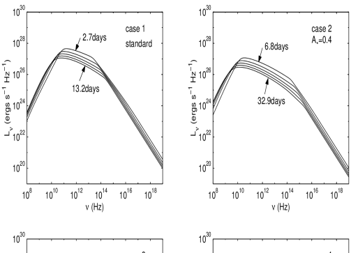
Figure 3: Lightcurves of the bow shock emission for six different cases (see §3 for details). In each case, the start and end times are labeled on the plot. The intermediate times are evenly distributed between the start and end times.

References

- (1)
- (2) Berger, E., et al. 2000, Astro-ph/0005465
- (3)
- (4) Blandford, R. D., & McKee, C. F. 1976, Phys. Fluids, 19, 1130
- (5)
- (6) Bloom, J. S. et al. 1999, Nature, 401, 453
- (7)
- (8) Chevalier, R. A. 1998, ApJ, 499, 810
- (9)
- (10) —————. 1999, ApJ, 511, 798
- (11)
- (12) Chevalier, R. A., & Li, Z. Y. 1999, ApJ, 520, L29
- (13)
- (14) —————————–. 2000, ApJ, 536, 195
- (15)
- (16) Costa, E., et al. 1997, Nature, 387, 783
- (17)
- (18) Dai, Z. G., Huang, Y. F. & Lu, T. 1999, ApJ, 520, 634
- (19)
- (20) Filippenko, A. V. 1997, ARA&A, 35, 309
- (21)
- (22) Folkes, S., et al. 1999, MNRAS, 308, 459
- (23)
- (24) Frail, D. A., Kulkarni, S. R., Nicastro, L., Feroci, M., & Taylor, G. B. 1997, Nature, 389, 261
- (25)
- (26) Fransson, C., Lundqvist, P., & Chevalier, R. A. 1996, ApJ, 461, 993
- (27)
- (28) Galama, T. J., et al. 1999, Astr. & Ap. S, 138, 465
- (29)
- (30) Garnavich, P. M., et al. 2000, ApJ, accepted (Astro-ph/0003429)
- (31)
- (32) Gaskell, C. M. 1992, ApJ, 389, L17
- (33)
- (34) Giacconi, R., et al. 2000, astro-ph/0007240
- (35)
- (36) Granot, J., Piran, T., & Sari, R. 1999, ApJ, 513, 679
- (37)
- (38) Halpern, J. P., et al. 2000, Astro-ph/0006206
- (39)
- (40) Harrison, F. A., et al. 1999, ApJ, 523, L121
- (41)
- (42) Jensen, B. L., et al. 2000, Astro-ph/0005609
- (43)
- (44) Katz, J. I. 1994, ApJ, 422, 248
- (45)
- (46) Khokhlov, A. M., Hoeflich, P. A., Oran, E. S., Wheeler, J. C., Wang, L. 1999, ApJ, 524, L107
- (47)
- (48) Koyama, K., et al. 1995, Nature 378, 255
- (49)
- (50) Koyama, K., et al. 1997, PSAJ, 49, L7
- (51)
- (52) Kulkarni, S. R., et al. 2000, to appear in Proc. of the 5th Huntsville Gamma-Ray Burst Symposium; astro-ph/0002168
- (53)
- (54) Li, Z. Y., & Chevalier, R. A. 1999, ApJ, 526, 716
- (55)
- (56) MacFadyen, A. I., Woosley, S. E., Heger, A. 1999, ApJ, submitted (astro-ph/9910034)
- (57)
- (58) Madau, P., Blandford, R. D., & Rees, M. J. 2000, ApJ, in press; astro-ph/9912276
- (59)
- (60) Masetti, N., et al. 2000, Astro-ph/0004186
- (61)
- (62) Mészáros, P., & Rees, M. J. 1993, ApJ, 405, 278
- (63)
- (64) ———————————–. 1997, ApJ, 476, 232
- (65)
- (66) Metzger, M. R., et al. 1997, Nature, 387, 879
- (67)
- (68) Muraishi, H. et al. 2000, A&A, in press; astro-ph/0001047.
- (69)
- (70) Paczyński, B., & Rhoads, J. E. 1993, ApJ, 418, L5
- (71)
- (72) Panaitescu, A., & Mészáros, P. 1999, ApJ, 526, 707
- (73)
- (74) Pian, E. 1999, Astro-ph/9910236
- (75)
- (76) Reichart, D. E. 1999, ApJ, 521, L111
- (77)
- (78) Rhoads, J. E. 1997, ApJ, 487, L1
- (79)
- (80) ————. 1999a, ApJ, 525, 737
- (81)
- (82) ————. 1999b, Astron. & Ap. Suppl., 138, 539
- (83)
- (84) Rybicki, G. B., & Lightman, A. P. 1979, Radiative Processes in Astrophysics (New York: Wiley Interscience), p. 147
- (85)
- (86) Sagar, R., Mohan, V., Pandey, S. B., Pandey, A. K., Stalin, C. S., & Castro-Tirado, A. J. 2000, Astro-ph/0004223
- (87)
- (88) Sari, R., Piran, T., & Narayan, R. 1998, ApJ, 497, L17
- (89)
- (90) Stanek, K. Z., Garnavich, P. M., Kaluzny, J., Pych, W., Thompson, I. 1999, ApJ, 522, L39
- (91)
- (92) Tanimori, T. et al. 1998, ApJ, 497, L25
- (93)
- (94) Umeda, H. 2000, ApJ, 528, L89
- (95)
- (96) van Paradijs, J., et al. 1997, Nature, 386, 686
- (97)
- (98) Vaughan, T. E., Branch, D., Miller, D. L., & Perlmutter, S. 1995, ApJ, 439, 558
- (99)
- (100) Wang, X., & Loeb, A. 2000, ApJ, 535, 788
- (101)
- (102) Waxman, E. 1997a, ApJ, 485, L5
- (103)
- (104) ———. 1997b, ApJ, 489, L33
- (105)
- (106) Wijers, R. A. M. J., Rees, M. J., & Mészáros, P. 1997, MNRAS, 288, L51
- (107)
- (108) Wijers, R. A. M. J., Bloom, J. S., Bagla, J. S., & Natarajan, P. 1998, MNRAS, 294, L13
- (109)
- (110) Woods, E., & Loeb, A. 1999, ApJ, submitted; astro-ph/9907110
- (111)
- (112) Young, T. R., & Branch, D. 1989, ApJ, 342, L79
- (113)
- (114) Zimmermann, H. U., et al. 1994, Nature, 367, 621
- (115)