A comparison of light and velocity variations in Semiregular variables

Abstract

NIR velocity variations are compared with simultaneous visual light curves for a sample of late-type semiregular variables (SRV). Precise radial velocity measurements are also presented for the SRV V450 Aql. Our aim is to investigate the nature of the irregular light changes found in these variables.

Light and velocity variations are correlated in all stars of our sample. Based on these results we discuss several possibilities to explain the observed behavior. We find that pulsation is responsible for large amplitude variations. In a recent paper Lebzelter (Lebzelter99 (1999)) invoked large convective cells to understand observed velocity variations. This possibility is discussed with respect to the observed correlation between light and velocity changes. In the light of these results we investigate the origin of the semiregular variations.

1 Introduction

The first discovery of semiregular light variation for a red giant ($\mu$ Cep) dates to 1782 (see Burnham Burnham78 (1978) for a historical review). Since that time an enormous amount of light curve data has been collected, with most of the data for large amplitude late-type variable (miras) coming from amateur astronomers. For the lower amplitude late-type variables a distinct group has been assigned, the semiregular variables (SRVs; Kholopov et al. 1985– (88), GCVS4).

In this paper we will focus on the semiregular subclasses SRa and SRb only, and exclude SRc (supergiants) and SRd (yellow giants). A comprehensive discussion of the properties of SRas and SRbs has been given by Kerschbaum & Hron (KH92 (1992), KH94 (1994)). The SRVs are evolved stars, probably located on the AGB; however their evolutionary status on the AGB is still a matter of debate (e.g. Lebzelter & Hron LH99 (1999)). The bluer SRVs, which typically also have the shorter periods, show less mass loss and no indications for thermal pulses. The redder SRVs have longer periods, and can show mass loss comparable to the miras.

The cause of the irregularities in the light variations of the SRVs is far from being understood. Recently, empirical evidence has been presented for multiple period changes (Mattei et al. MFH98 (1998), Kiss et al. KSCM99a (1999)), which may be due to many (2 or more) simultaneously excited modes of pulsation. The observed mode changes in several semiregular stars (Cadmus et al. CWSM91 (1991), Percy & Desjardnis PD96 (1996), Bedding et al. BZJF98 (1998), Kiss et al. KSCM99a (1999)) strongly suggest a pulsational origin for the multiperiodic nature. However, other explanations, e.g. chaotic phenomena (Aikawa Aikawa87 (1987), Icke et al. IFH92 (1992)) perhaps in combination with an interplay of excited modes of pulsation (Buchler & Goupil BG88 (1988)) or coupling of rotation and pulsation (Barnbaum et al. BMK95 (1995)) have been suggeested in the literature. One has to be aware that all of these mechanisms may simply be cases of ‘chaos’ (see e.g. Buchler & Kolláth BK00 (2000)). Further explanations include dust-shell dynamics (Höfner et al. HFD95 (1995)) or large convective cells (Antia et al. ACN84 (1984)). Observed spatial asymmetries in some Mira variables (Karovska Karovska99 (1999)) could imply the possibility of non-radial oscillations. This was also discussed as an explanation for the amplitude modulation of the SRb-type variable RY UMa (Kiss et al. KSSM99b (2000)).

A problem in understanding the nature of the SRVs is that nearly all observations have been of visual colors. To develop a physical model for the SRV changes, monitoring of time variability of other parameters like velocity or temperature variations is needed. One approach is to monitor the velocity variations of SRVs closer to the pulsation driving zone through time-series high-resolution infrared spectroscopy. Hinkle et al. (HLS97 (1997)) and Lebzelter (Lebzelter99 (1999)) reported on time-series high-resolution spectroscopy of second overtone and high excitation first overtone CO lines located in an opacity minimum around 1.6 $\mu$m. However, in both papers only phase information (relative to a close light curve maximum) was used to search for regularities in the velocity variations and to derive an amplitude of the velocity curve. As the variations in SRVs are far from being regular both in the sense of period length as well as amplitude, a phase estimated in this way may significantly misrepresent the behavior of the light curve.

A direct comparison between light and velocity changes has been done for the mira variable $χ$ Cyg (Hinkle et al. HHR82 (1982)). The velocity curves of miras are all similar and discontinuous with an amplitude of 20 to 30 km/s. Line doubling is observed around maximum light, and at that phase typically both maximum and minimum velocity occur. Around phase 0.4, i.e. shortly before light minimum, the velocity curve reaches the center-of-mass velocity. This point in the variability cycle might therefore be related to the maximum expansion of the layer producing the CO lines used to derive the velocity curve. Other miras show similar results; the velocity amplitudes of SRVs are significantly less (Hinkle et al. HSH84 (1984), Hinkle et al. HLS97 (1997)).

This paper is dedicated to the irregularities. We will compare simultaneously measured light and velocity curves to correlate the irregularities. The velocity variations represent the movement of atmospheric layers due to stellar pulsation. In this way we will investigate whether the irregularities in the light curve are due to nonregular pulsation or due to surface structures like active regions or velocity fields introduced by convective cells.

2 Observations

2.1 Velocity variations

Most of the velocity data of SRVs that will be discussed have been published elsewhere (Hinkle et al. HLS97 (1997), Lebzelter Lebzelter99 (1999)). We selected stars that have a reasonable number of velocity and light curve measurements. For comparison we have also included the short period mira RT Cyg. This star has a period similar to the SRVs but with a significantly larger amplitude in V. The velocity amplitude is also similar to that of other miras (Lebzelter et al. LHH99 (1999)). The final sample covers a large range in period and amplitude. Both types, SRa and SRb, are included. Table 1 gives an overview on the origin of the data and the instruments used to obtain them as well as fundamental properties of the stars.

Table 1: Properties of stars selected for the present investigation. Column 3, 4, 5 and 6 give general properties of the objects from the GCVS4. Column 7 and 8 list the source of the velocity data, where CF stands for the Coudé Feed telescope on Kitt Peak. References are encoded as follows: HLS97 = Hinkle et al. 1997; LHH99 = Lebzelter et al. 1999; LZ99 = Lebzelter 1999.

Object	IRAS	GCVS data				velocity data
	name	type	spectrum	period [d]	V ampl. [mag]	reference	instrument
Aql V450	19312+0521	SRb	M5	64.2	0.35	this paper	FTS KPNO
Cas SV	23365+5159	SRa	M6	265	3.4	HLS97	FTS KPNO
Cyg W	21341+4508	SRb	M4-6	131	2.1	HLS97	FTS KPNO
Cyg RT	19422+4839	M	M2-8.8	190	7.1	LHH99	FTS KPNO
Cyg RU	21389+5405	SRa	M6e	233	1.4	HLS97	FTS KPNO
Dra TX	16342+6034	SRb	M4e-5e	78	2.3	LZ99	CF + NICMASS
Her g	16269+4159	SRb	M6	89	2.0	LZ99	CF + NICMASS
Her ST	15492+4837	SRb	M6-7	148	1.5	LZ99	CF + NICMASS
Hya W	13462-2807	SRa-M	M8e	382	3.9	HLS97	FTS KPNO

FTS spectra were obtained over a broad wavelength interval always covering the entire 1.6 $\mu$m H window and frequently the entire 1.6-2.5 $\mu$m H and K region. We present a single velocity from these measurements. The Coudé Feed spectrograph with the NICMASS detector covers a very small spectral region, about 2 percent of the H band window (Lebzelter Lebzelter99 (1999)). The Coudé Feed observations were always obtained in two wavelength regions, both around 1.6 $\mu$m, that were analyzed separately. In the figures of this paper these two sets of NICMASS observations will be marked by two different symbols.

Previously unpublished velocity data for the semiregular variable V450 Aql are also presented. Observations were obtained with the FTS at the 4 m Mayall telescope on Kitt Peak. The data are listed in Table 2. Details on the data reduction techniques can be found in Hinkle et al. (HHR82 (1982)). The excitation temperature and column density were derived from the CO lines for two observations as described in Hinkle et al. (HHR82 (1982)). As has been found for other similar SRVs, the uncertainty of these numbers (T_exc=3300$\pm$200 and log(NL[CO])=22.8$\pm$0.1) is too large to allow derivation of stellar variations in low amplitude variables.

Some confusion is found in the literature concerning the spectral type of V450 Aql. Most authors agree that the spectral type is M5 to M5.5III (e.g. Keenan & McNeil KM89 (1989)), while the Hipparcos Input Catalogue lists M8V, apparently based on a measurement by McCuskey (McCuskey49 (1949)). From its IRAS colours V450 Aql clearly belongs to the blue SRVs (Kerschbaum & Hron KH92 (1992)).

Table 2: FTS measurements for V450 Aql. Spectra have been apodized by Norton & Beer (NB76 (1976)) function I2. Resolution (theor. FWHM) of the spectra is 0.07 cm^-1.

JD	S/N	integration	radial	number
2440000+		time [min]	velocity [km/s]	of lines
5604.7	76	110	$-$52.34$\pm$0.14	76
5752.3	61	34	$-$52.98$\pm$0.12	74
5776.2	48	42	$-$52.90$\pm$0.10	75
5782.2	62	34	$-$52.72$\pm$0.11	74
5799.1	69	51	$-$53.79$\pm$0.12	74
5812.1	52	34	$-$53.62$\pm$0.15	76
5837.1	58	56	$-$53.63$\pm$0.11	78
5841.0	43	50	$-$53.89$\pm$0.09	79
6005.5	52	50	$-$52.32$\pm$0.16	76
6018.4	85	67	$-$52.51$\pm$0.12	73

The literature values for the radial velocity of V450 Aql scatter between $-$52 km/s (Feast, Woolley & Yilmaz FWY72 (1972)) and $-$50.6 km/s (Jones & Fisher JF84 (1984)). We will use an average value of $-$51.3 km/s. All velocity measurements we obtained for this object (Table 2) are slightly below this literature value. V450 Aql therefore exhibits the same behavior found already for a number of SRVs by Lebzelter (Lebzelter99 (1999)), namely a systematic shift between the literature values and the measured CO velocities.

2.2 Light curve data

The measurement and long-term monitoring of long-period variable magnitudes is one field in astronomy where the contribution of amateur astronomers is crucial. The investigation presented in this paper was made possible by the rich data base of individual magnitude estimates provided by associations of amateur astronomers. Three sources of visual data were utilized, namely those of the Association Francaise des Observateurs d’Etoiles Variables (AFOEV), the Variable Star Observers’ League in Japan (VSOLJ) and the American Association of Variable Star Observers (AAVSO International Database which includes part of AFOEV and VSOLJ observations). The possible effects of overlapping data series (i.e. the common estimates can be included twice or thrice) were avoided, because where the (most complete) AAVSO data were available we did not mix them with the other ones. On the other hand, there are practically no common observations in the AFOEV and VSOLJ data base.

In order to decrease the effects of the observational scatter, we applied similar data handling as used in Kiss et al. (KSCM99a (1999)). That means data averaging in 5- or 10-day bins depending on the actual period value. Further noise-filtering was done by applying a Gaussian smoothing with a FWHM of 4 and 8 days (80 percent of the bin). This was necessary in the very low-amplitude regime, where the usual accuracy of individual estimates (about $\pm$0.3 mag) would obscure the light variations. The use of this smoothing was illustrated in a comparison with simultaneous photoelectric measurements (see Fig. 2 in Kiss et al. KSCM99a (1999)) and turned out to be very effective in the case of light curves with numerous and densely distributed data. The estimated precision (in the visual system) is somewhat better than 0.1 mag. However, since there are no independent and simultaneous well-calibrated photometric data, the accuracy can only be estimated.

3 Results

In Figs. 1 to 9 we plotted the velocity variations on top of the light variations. For some stars single velocity data points from a few years earlier exist. These were not included in the plots to allow for a larger scale on the time axis. A mean velocity of the star – when available – has been subtracted from the velocity values. The velocity used for subtraction is given in the figure caption. Lebzelter (Lebzelter99 (1999)) found that thermal CO velocities and other values from the literature all appeared to share the same property, i.e. a systematic offset in the sense that the IR CO lines are blueshifted for all or a large part of the lightcycle. We will come back to this point in the discussion of the results. Note that some of these stellar velocities have been derived from blue/optical spectra and may therefore not be representative of the center-of-mass velocity. For miras it has been shown that the blue/optical velocities are shifted several km s^-1 positive of the center-of-mass velocity (Reid Reid76 (1976), Hinkle & Barnes HB79 (1979)). Wallerstein & Dominy (WD88 (1988)) found for 5 semiregular variables without H₂O masers that on the average there is no velocity shift between optical and thermal (=systemic) velocity. However, for 4 SRVs in their sample showing H₂O maser emission a difference v_thermal $-$ v_optical of $-$1.3 km/s was found. It is therefore not clear whether the optical velocity is representative for the center-of-mass velocity or not.

However, as thermal CO velocities are missing for many objects, the velocities used here are the only external source of velocity information available. Keeping the above mentioned uncertainty in mind we will use this velocity value as systemic velocity. We note that an investigation of a systematic velocity shift between blue and thermal CO velocities is still missing for semiregular variables. To avoid confusion we will add a remark on the source of the velocity in the figure caption (thermal CO or blue/optical). For the reference of each velocity we refer to the paper listed in Table 1.

The velocities have been plotted in reverse order (largest velocity at the bottom) for the sake of an easier comparison of velocity and light variations. Throughout this paper positive velocity relative to the systemic velocity means that the material is moving toward the star and hence away from the observer. Furthermore the scale of the velocity axis has been adjusted to have an overlap between velocity and light curve.

It is obvious that the light and velocity variations are well correlated in all objects of our sample. Some – but not all – changes in the light amplitude are well represented in the behavior of the velocity curve as well. All stars reach their smallest difference to the systemic velocity at or close to light minima, while the minimum velocities are correlated with light maxima.

V450 Aql exhibits velocity changes with an amplitude of about 1.6 km/s. This is the smallest variation in our sample and one of the smallest among the stars for which Hinkle and collaborators monitored CO velocities. The accuracy of the velocity measurements is high enough to ensure that the star is truly variable in velocity. However, due to the small amplitude the uncertainties in the light curve and the sampling of our velocity measurements makes comparison of light and velocity curve rather difficult (Fig. 1). Although it seems like V450 Aql behaves the same way as all the other stars, even the opposite behavior (i.e. maximum velocity at maximum light) cannot be excluded.

Line doubling is present in the short period mira RT Cyg (Fig. 5) significantly before the visual light maximum. If we compare the behavior of this star with the velocity curve of $\chi$ Cyg, we have to keep in mind that RT Cyg has a very symmetric light curve compared to its long period counterpart. The slight phase shift between the minimum velocity and the light maximum found in $\chi$ Cyg is not visible in RT Cyg. However, it is possible that the phase coverage is not adequate to detect such a small shift (which we would expect to be only a few days due to RT Cyg’s short period). Light curve data do not allow a determination of the exact date of minimum around JD 2446200. Still the line doubling observation with the maximum velocity observed seems to be located clearly after the light minimum in agreement with the pattern seen in $\chi$ Cyg. The single velocity measurement two cycles later fits very well onto the light curve as well indicating that the correlation of light and velocity curve is not limited to the well covered period.

The data for SV Cas (Fig. 2) also merit further comments. The behavior of this star was difficult to interpret without the light curve. Plotting all data into one cyle made Hinkle et al. (HLS97 (1997)) suspect that the star might have a velocity curve similar to the miras, i.e. discontinuous. Our result shows that this interpretation is not necessary, because the velocity variations follow the semiregular light variations quite well. It was incomplete phase coverage of the velocity observations that led to the misinterpretation. The three maxima visible in Fig. 2 give a mean period of only 237 days, somewhat less than the GCVS4 value used by Hinkle et al.

The comparison of parallel velocity and light variations is of similar importance for the understanding of the velocity variations in the case of ST Her (Fig. 8). Lebzelter (Lebzelter99 (1999)) assumed a phase shift between the velocity measurements around JD 2450150 and earlier data points to explain that the velocities did not fit into a simple phase diagram. Fig. 8 shows that this assumption was correct and that the star is not following its mean period around that day. However, the velocities around that time fit well onto the observed light curve.

Figure 1: Light and velocity variations of V450 Aql. Filled circles mark velocity measurements (right axis). No error bars are given as the error bar would be typically of the size of the symbols as can be easily seen from Table 2. The stellar velocity ($-$51.3 km/s from blue/optical spectra, see text) has been subtracted. To allow a better comparison velocity axis is in reverse order. Light curve data points are labeled with crosses.

Figure 2: Light and velocity variations of SV Cas. For this star no center-of-mass velocity is available in the literature. Therefore absolute velocity values are plotted. Same symbols as in Fig.  1.

Figure 3: Light and velocity variations of W Cyg. Stellar velocity ($-$14.4 km/s from thermal microwave CO, see Hinkle et al. HLS97 (1997)) has been subtracted from the velocity data. Same symbols as in Fig.  1.

Figure 4: Light and velocity variations of RU Cyg. Stellar velocity ($-$6.3 km/s from thermal microwave CO, see Hinkle et al. HLS97 (1997)) has been subtracted from the velocity data. Same symbols as in Fig.  1.

Figure 5: Light and velocity variations of the short period mira RT Cyg. Stellar velocity ($-$118 km/s from blue/optical spectra, see Lebzelter et al. LHH99 (1999)) has been subtracted from the velocity data. The arrows indicate the phase of line doubling. Same symbols as in Fig.  1.

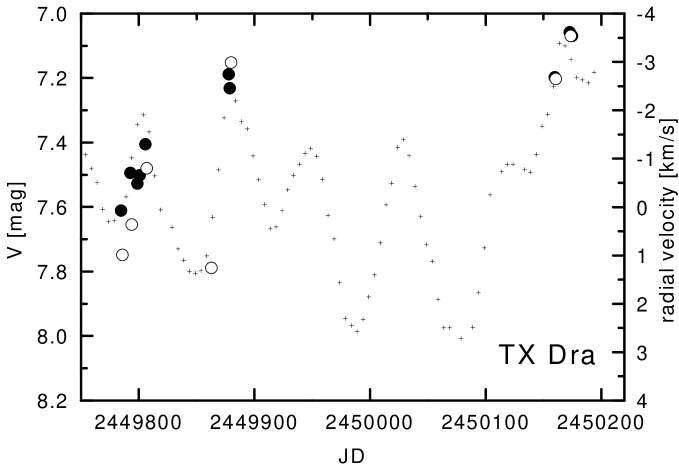
Figure 6: Light and velocity variations of TX Dra. Stellar velocity (46.4 km/s from blue/optical spectra, see Lebzelter Lebzelter99 (1999)) has been subtracted from the velocity data. Velocity has been measured in two wavelength regions (see text). Wavelength region 1 is marked by filled circles, wavelength region 2 by open circles.

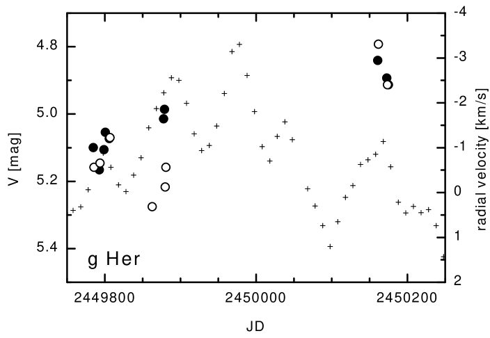
Figure 7: Light and velocity variations of g Her. Stellar velocity (1.4 km/s from thermal microwave CO, see Lebzelter Lebzelter99 (1999)) has been subtracted from the velocity data. Same symbols as in Fig.  6.

For four additional stars (RV Boo, RR CrB, X Her, and TT Dra) velocities are available but good light curves are not, making a detailed comparison, as for the stars in Table 1, impossible. Using available light curves, we attempted to confirm that these stars behave as the stars with good light curves. All of them seem to exhibit the same kind of correlation between light and velocity changes.

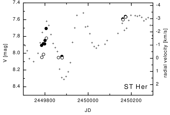
Figure 8: Light and velocity variations of ST Her. Stellar velocity ($-$22 km/s from thermal microwave CO, see Lebzelter Lebzelter99 (1999)) has been subtracted from the velocity data. Same symbols as in Fig.  6.

Figure 9: Light and velocity variations of W Hya. Stellar velocity (38 km/s from thermal microwave CO, see Hinkle et al. HLS97 (1997)) has been subtracted from the velocity data. Same symbols as in Fig.  1.

4 Discussion

4.1 The relation between light and velocity changes

From the figures it is obvious that the light and velocity changes in semiregular variables are correlated. Most of the light curve irregularities, especially variability in the length of a cycle, are physically linked to a ”semiregular” velocity curve. A relation between the size of light and velocity change is indicated by comparison of the velocity amplitude and light amplitude listed in GCVS4 (Hinkle et al. HLS97 (1997)). By using the light curves there is the possibility for a more direct comparison of these two quantities.

Might it be possible to quantify the qualitative impression of the relation between light and velocity changes? Such an attempt is of course restricted by the limited accuracy both in the light curve and in the velocity data, and the small time span covered by the observations. Therefore we consider the following result as preliminary. The comparison of light and velocity amplitudes by Hinkle et al. (HLS97 (1997)) gives a mean ratio between light and velocity change of approximately 4 km/s/mag for the semiregular variables. However, our comparison of simultaneously obtained velocity and light measurements shows that the ratio ranges from 3 to 7 km/s/mag. (For V450 Aql and g Her we did not derive this quantity as velocity and light changes do not correlate as well as the other objects in our sample.) Most of the scatter will originate from the lower time resolution of the velocity data leaving considerable uncertainty in shifting and scaling the velocity curve onto the light curve. While the order of the mean value of both investigations is the same, the large scatter we found in the more detailed comparison indicates a more complex relation between velocity and light change as the latter will be influenced by other parameters, for example temperature variations. Data on bolometric light variations and simultaneous information on the temperature change would be necessary to allow a better quantification of such a relation. Furthermore, due to the obvious changes from cycle-to-cycle the definition of a mean amplitude and an amplitude range will be the more appropriate parameter.

Cummings et al. (CHKG98 (1998)) presented high-precision relative radial velocities measured in the optical wavelength region for 31 red giants. They also made broad-band photometric observations to differentiate between possible causes of velocity variations. The observed light and radial velocity variations were either in inverted phase, or shifted by a significant percentage (up to 30-40%) of the cycle-length. What they found is in good agreement with our results.

4.2 Indications for the cause of the variability

When identifying the mechanism responsible for the observed variations two features visible in the data must be taken into account. First, all SRVs show their maximum velocity at light minimum and their minimum velocity at light maximum. Second, most of the SRVs investigated here show the puzzling feature that the measured CO velocities are all more negative then the stellar velocity (Lebzelter Lebzelter99 (1999)).

4.2.1 Velocity shift

The observed velocity shift between the high excitation CO lines and the systemic velocity has been mentioned already in Lebzelter (Lebzelter99 (1999)). For some stars the velocity reference point has been obtained from blue-optical spectra. While it is not clear whether this spectral range is useable to determine the systemic velocity or not, we note that the same effect is observed for stars, for which the center-of-mass velocity has been derived from microwave thermal CO observations.

Several mechanisms are thinkable for producing such a velocity shift. Some of them have already been discussed by Lebzelter (Lebzelter99 (1999)). Pulsation may well produce considerable velocity shifts and asymmetries between maximum outflow and infall velocity. It has been shown from model calculations of AGB stars that traveling waves introduced by the pulsation can persist longer than one light cycle in the stellar atmosphere (e.g. Höfner & Dorfi HD97 (1997)). These effects are correlated with the strength of the pulsation. As the objects discussed here are mainly low amplitude objects it is not clear yet, if a velocity shift of correct size can be produced by pulsation alone. Models of late type pulsating stars calculated by Bowen (Bowen88 (1988)) indicate the existence of a warm ”chromospheric” layer of outflowing gas (called ”calorisphere” by Willson & Bowen WB86 (1986)). If the CO lines we use in this investigation are formed in such a layer then its outward motion may well explain the observed velocity shift. However, the high excitation CO lines are quite weak, so it is more likely that they are formed deep inside the stellar atmosphere. Furthermore, such a layer is not found in the models by Höfner & Dorfi (HD97 (1997)), therefore its existence is still a matter of debate. A further possible mechanism responsible for the velocity shift are large convective cells on the stellar surface as suggested by Lebzelter (Lebzelter99 (1999)). However, detailed modeling of variability due to stellar convection is not yet available for AGB stars.

In the following we will discuss the correlation between light and velocity changes in the light of the possible reasons accounting for the velocity shift.

4.2.2 Pulsation

In this section we discuss the case when the pulsation is considered to be the dominant factor in producing stellar light and velocity changes. In the case of variations driven only by pulsation an assumption must be made to deal with the systematic difference between the observations and the center-of-mass velocity. Possible reasons have been mentioned above and in Lebzelter (Lebzelter99 (1999)). However, the further discussion does not depend on what reason is chosen.

Superficially both the light curves and radial velocity curves are in agreement with radial pulsation being the main reason for the light variations. The observed properties, e.g. radial velocity minima occurring very close to maximum light, are typical in radially pulsating stars (RR Lyrae-, high-amplitude $\delta$ Scuti- and Cepheid variables). In radially pulsating stars the light- and radial velocity curves are in some cases perfectly mirror images (see e.g. Bersier et al. 1994a , 1994b ). Our velocity curves are plotted in an inverted form, therefore, they show exactly the same behavior as other radial pulsators. This means that the star reaches its maximum light during the expansion.

However, such a ’mirror behavior’ suggests that the light variation is caused by radius variation only. From miras we know that the visual light change in late-type stars is dominated by the temperature change via the variations in the strengths of the TiO bands. The effect of the TiO bands is exactly the opposite way, leading to a minimum flux (in the visual) when the star is largest, i.e. has its minimum temperature. In that case a phase shift between the CO line forming layers and the layers producing the visual continuum is necessary to explain the observations reported in this paper. This is in agreement with results from present AGB star models proposing extended atmospheres where different spectral features can originate at completely different radii from the stellar center. Unfortunately, no simultaneous temperature determinations exist for the SRVs of our sample.

Accepting this pulsational approach, we estimated the order of magnitude of the relative radius variation caused by the radial motion. A well observed example is W Cygni. W Cygni’s light curve is dominated by two periods ($P_{0}=240$ days, $P_{1}=130$ days, Kiss et al. KSCM99a (1999)). These periods, their ratio and theoretical calculations by Ostlie & Cox (1986) imply the following stellar parameters: $M=1.4M_{\odot}$, $L=7000L_{\odot}$, $T=3000K$. The adopted model gives $P_{0}=238$ days and $P_{1}=129$ days for the fundamental and first overtone mode, respectively. Recent models including the coupling with convection (Xiong et al. XDC98 (1998)) give $P_{1}=230$ days and $P_{3}=130$ days (first and third overtones) for $M=1.0M_{\odot}$, $L=5000L_{\odot}$ and $T=2700K$. In either case the periods fit for a stellar radius of $\approx 300R_{\odot}$. Considering the data subset around JD 2446000, the radial velocity of W Cygni changed approximately 2 km s^-1 in 70 days which gives an order-of-magnitude estimate for the corresponding radial displacement about $\sim 17R_{\odot}$. That is 5 percent relative radius change being a reasonable value for a radial pulsator. This is, of course, a very oversimplified estimation. We stress that several different layers with different velocities might contribute to the final CO line profiles and hence to the measured velocities. Therefore radius variations calculated from these velocity variations have to be taken with care (see e.g. Hinkle et al. HHR82 (1982) for a discussion). However, the most important consequence of our simple estimate is that radial pulsation is a realistic explanation for a set of semiregular variables.

4.2.3 Convective cells

As a second approach we assume that the outer atmospheric layers do not pulsate at all. The velocity variations might then originate from convective motion. According to Schwarzschild (Schwarzschild75 (1975)) and other authors only a small number of convective cells cover the surface of an evolved red giant. Lebzelter (Lebzelter99 (1999)) suggested that they might be responsible for a systematic blueshift of the measured velocities. This is based on the assumption that we mainly see the outflowing matter which is hotter and therefore brighter than the matter flowing back onto the star. This outflow has to be by no means constant from the (distant) observers view. While the individual motion within each granule on a star like the sun will average out over the whole stellar disk, the situation is different for the red giants due to the small number of cells on the surface. Beside velocity variations within each individual cell the movement of cells on the stellar surface as well as their evolution will lead to significant variations both in light and velocity integrated over the stellar disk. Velocity variations caused by convective motion are also in agreement with the observed coincidence of maximum outflow velocity and light maximum. If the number of convective cells on the surface increases, the area of matter falling back onto the star, which forms the borders of these cells, increases. Therefore the fraction of the surface covered by infalling matter changes the brightness and the convective velocity shift in the same way. For a velocity variation within an individual convective cell the same effect is achieved as a higher velocity will carry hot matter into higher regions of the atmosphere leading to a brightening of the whole star. To quantify this, detailed simulations are needed. The time scale of the observed variations for the short period objects is in agreement with the convective time scale of about 40 days as noted by Antia et al. (ACN84 (1984)).

5 Variability of semiregular variables

The current data are not sufficient to determine the cause of irregular variations in late type stars. These irregular variations have been found in semiregular, irregular and mira-type variables. The irregularities found in mira velocity curves are of similar size to the velocity variations in the short period SRVs (see the data for $\chi$ Cyg in Hinkle et al. HHR82 (1982)) and might have a common cause.

We showed that both pulsation and convective cells can in principle produce velocity and light changes. The standard pulsation interpretation is in nice agreement with the observed correlation of velocity and light changes. On the other hand it is very difficult to estimate the size of the light and velocity variations due to convective cells without detailed modelling. The interesting feature of convective cells is the irregular variability and the systematic velocity shift they produce.

There are several features found in semiregular variables that cannot be explained without the assumption of stellar pulsation. A number of SRVs like W Hya have periods a few times the timescale estimated for convective cells. Furthermore, their rather large velocity amplitude and the crossing of the center-of-mass velocity by the velocity curve make an explanation with convective cells alone for the long period objects rather unlikely. It has also to be kept in mind that several semiregular variables at least sometimes show hydrogen emission lines of the Balmer series in their spectra. In the miras, and presumably in the SRVs, this emission component originates from shock waves in the stellar atmospheres. These shock waves are the result of global stellar pulsation, giving a strong argument for a pulsational origin for the light curve and velocity variations.

Models predict the existence of large convective cells at the surface of red giants. It is therefore very likely that the observed variability in light and velocity includes a component provided by these surface structures. This component will be found among small amplitude irregulars as well as among miras and may account for the fact that many ’nonvariable’ red giants are actually variables with small amplitudes (see e.g. Jorissen et al. JMSM97 (1997)). If one wants to explain this small amplitude variability with the help of large convective cells it is critical to know the center-of-mass velocity very accurately. Variability due to convective cells only should lead to a measured velocity smaller than the center-of-mass velocity (i.e. always outflow of matter) at all phases.

It is well known that miras do not always reach the same brightness in each light maximum. The differences (see e.g. Fig. 5) can be of the order of one magnitude. Such ’irregularities’ may be produced by processes on longer time scales than the main stellar pulsation period (e.g. Höfner & Dorfi HD97 (1997)). This illustrates that pulsation itself, even if only one mode is excited, can introduce irregularities into the light change of long period variables.

At the moment it is not possible to estimate whether convective motion can introduce the observed irregularity into the light and velocity changes alone or not. The variability of the objects with the smallest amplitudes might be explained by convective motion only. For those cases it does not seem necessary to explain the small scale variability with the help of high degree overtone modes as suggested by Percy & Parkes (PP98 (1998)). However, with the actual data available we cannot exclude regular pulsation or chaotic behavior in these objects, but we want to support the possibility of surface structures caused by convective motion as an alternative explanation.

To summarize, we think it is a reasonable approach to see the observed variability in semiregular and irregular variables as a composite of pulsation and an (additional?) irregularity introduced by, e.g., large convective cells. The importance of each of these two components will probably be very different for different objects.

A significant challenge for the late type variables is to define the regions of instability on the H-R diagram. If we want to have a chance to define the limiting parameters for the onset of pulsation and to estimate the influence of convective motion on the variability, a significantly larger sample of light and velocity curves as well as other stellar characteristics (both fundamental as well as atmospheric, for instance the occurrence of emission lines) are needed. In this context the light curves provided by amateur astronomers are of great value but they are not accurate enough to avoid ambiguities in small light curve irregularities. Therefore only photoelectric data as provided e.g. by automatic telescopes can reveal these details in the light curves. Both sources of data are needed to search for possible further components contributing to the light change of semiregular and irregular variables.

- (1) Aikawa T. 1987, Ap&SS 139, 281
- (2) Antia H.M., Chitre S.M., Narasimha D. 1984, ApJ 282, 574
- (3) Barnbaum C., Morris M., Kahane C. 1995, ApJ 450, 862
- (4) Bedding T.R., Zijlstra A.A., Jones A., Foster G. 1998, MNRAS 301, 1073
- (5) Bersier D., Burki G., Burnet M. 1994a, A&A Suppl. 108, 9
- (6) Bersier D., Burki G., Mayor M., Duquennoy A. 1994b, A&A Suppl. 108, 25
- (7) Bowen G.H. 1988, ApJ 329, 299
- (8) Buchler J.R., Goupil M.J. 1988, A&A 190, 137
- (9) Buchler J.R., Kolláth Z. 2000 in: “Nonlinear Stellar Pulsation”, Astrophysics and Space Science Library (ASSL), eds. M. Takeuti & D. Sasselov, in press
- (10) Burnham R. 1978, Burnham’s Celestial Handbook, Dover Publications Inc., New York
- (11) Cadmus R.R., Willson L.A., Sneden C., Mattei J.A. 1991, AJ 101, 1043
- (12) Cummings I.N., Hearnshaw J.B., Kilmartin P.M., Gilmore A.C. 1998, In:“A Half-Century of Stellar Pulsation Interpretations”, eds. P.A. Bradley and J. Guzik, ASP Conf. Series 135, p.213
- (13) Feast M.W., Woolley R., Yilmaz N. 1972, MNRAS 158, 23
- (14) Hinkle K.H., Barnes T.G. 1979, ApJ 234, 548
- (15) Hinkle K.H., Hall D.N.B., Ridgway S.T. 1982, ApJ 252, 697
- (16) Hinkle K.H., Scharlach W.W.G., Hall D.N.B. 1984, ApJ Suppl. 56, 1
- (17) Hinkle K.H., Lebzelter T., Scharlach W.W.G. 1997, AJ 114, 2686
- (18) Höfner S., Dorfi E.A. 1997, A&A 319, 648
- (19) Höfner S., Feuchtinger M.U., Dorfi E.A. 1995, A&A 297, 815
- (20) Icke V., Frank A., Heske A. 1992, A&A 258, 341
- (21) Jones D.H.P., Fisher J.L. 1984, A&A Suppl. 56, 449
- (22) Jorissen A., Mowlavi N., Sterken C., Manfroid J. 1997, A&A 324, 578
- (23) Karovska M. 1999, Proc. IAU Symp. 191, “Asymptotic Giant Branch Stars”, eds. T. Le Bertre, A. Lebre and C. Waelkens, p.139
- (24) Keenan P.C., McNeil R.C. 1989, ApJ Suppl. 71, 245
- (25) Kerschbaum F., Hron J. 1992, A&A 263, 97
- (26) Kerschbaum F., Hron J. 1994, A&A Suppl. 106, 397
- 1985– (88) Kholopov P.N., Samus N.N., Frolov M.S., et al. 1985–88, General Catalogue of Variable Stars, edition, “Nauka” Publishing House, Moscow (GCVS4)
- (28) Kiss L.L., Szatmáry K., Cadmus Jr. R.R., Mattei J.A. 1999, A&A 346, 542
- (29) Kiss L.L., Szabó Gy., Szatmáry K., Mattei J.A., 2000, Proc. IAU Coll. 176 “The impact of large-scale surveys on pulsating star research”, eds. L. Szabados & D. Kurtz, ASP Conf. Series, in press
- (30) Lebzelter T. 1999, A&A 351, 644
- (31) Lebzelter T., Hron J. 1999, A&A 351, 533
- (32) Lebzelter T., Hinkle K.H., Hron J. 1999, A&A 341, 224
- (33) Mattei J.A., Foster G., Hurwitz L.A., et al. 1998, In: the Proceedings of the ESA Symposium Hipparcos - Venice’97, ESA SP-402, p.269
- (34) McCuskey S.W. 1949, ApJ 109, 426
- (35) Norton R.H., Beer R. 1976, J.Opt.Soc.Am. 66, 259
- (36) Ostlie D.A., Cox A.N. 1986, ApJ 311, 864
- (37) Percy J.R., Desjardnis A. 1996, PASP 108, 847
- (38) Percy J.R., Parkes M. 1998, PASP 110, 1431
- (39) Reid M.J. 1976, ApJ 207, 784
- (40) Schwarzschild M. 1975, ApJ 195, 137
- (41) Wallerstein G., Dominy J.F. 1988, ApJ 326, 292
- (42) Willson L.A., Bowen G.H. 1986, in: Lecture Notes in Physics, vol. 254, Cool Stars, Stellar Systems and the Sun, ed. M.Zeilik & D.M.Gibson, p.385
- (43) Xiong D.R., Deng L., Cheng Q.L. 1998, ApJ 499, 355