Monte Carlo simulations of star clusters – II. Tidally limited, multi–mass systems with stellar evolution.

Abstract

A revision of Stodółkiewicz’s Monte Carlo code is used to simulate evolution of large star clusters. The new method treats each superstar as a single star and follows the evolution and motion of all individual stellar objects. A survey of the evolution of $N$–body systems influenced by the tidal field of a parent galaxy and by stellar evolution is presented. The process of energy generation is realised by means of appropriately modified versions of Spitzer’s and Mikkola’s formulae for the interaction cross section between binaries and field stars and binaries themselves. The results presented are in good agreement with theoretical expectations and the results of other methods (Fokker–Planck, Monte Carlo and $N$–body). The initial rapid mass loss, due to stellar evolution of the most massive stars, causes expansion of the whole cluster and eventually leads to the disruption of less bound systems ($W_{0}=3$). Models with larger $W_{0}$ survive this phase of evolution and then undergo core collapse and subsequent post-collapse expansion, like isolated models. The expansion phase is eventually reversed when tidal limitation becomes important. The results presented are the first major step in the direction of simulating evolution of real globular clusters by means of the Monte Carlo method.

1 INTRODUCTION.

Understanding the dynamical evolution of self–graviting stellar systems is one of the grand challenges of astrophysics. Among its many applications, the one which motivates the work presented here is the study of real globular clusters. Unfortunately, dynamical modelling of globular clusters and other large collisional stellar systems (like galactic nuclei, rich open clusters and galaxy clusters) still suffers from severe drawbacks. These are, on the one hand, due to the very high (and presently unfulfilled) hardware requirements needed to model realistic, large stellar systems by use of the direct $N$–body method, and partly due to the poor understanding of the validity of assumptions used in statistical modeling based on the Fokker–Planck and other approximations. The Fokker–Planck method with finite differences, which has recently been greatly improved, can now be used to simulate more realistic stellar systems. It can tackle: anisotropy, rotation, a tidal boundary, tidal shocking by galactic disk and bulge, a mass spectrum, stellar evolution and dynamical and primordial binaries (Takahashi 1995, 1996, 1997, Takahashi & Portegies Zwart 1998, 1999 hereafter TPZ, Drukier et al. 1999, Einsel & Spurzem 1999, Takahashi & Lee 1999 ). Unfortunately, the Fokker–Planck approach suffers, among other things, from the uncertainty of differential cross–sections of many processes which are important during cluster evolution. It can not supply detailed information about the formation and movement of all objects present in clusters. Additionally, the introduction of the mass function, mass loss and tidal boundary into the code is very approximate. Direct $N$–body codes are the most natural methods that can be used in simulations of real star clusters (NBODY – Aarseth 1985, 1999a, 1999b, Spurzem & Aarseth 1996, Portegies Zwart et al. 1998 – KIRA). They practically do not suffer from any restrictions common in the Fokker–Planck method. But unfortunately, even special–purpose hardware (Makino et al al. 1997 and references therein) can be used effectively only in $N$–body simulations which are limited to a rather unrealistic number of stars (i.e. too small for globular clusters). Another possibility is to use a code which is very fast and provides a clear and unambiguous way of introducing all the physical processes which are important during globular cluster evolution. Monte Carlo codes, which use a statistical method of solving the Fokker–Planck equation, provide all the necessary flexibility. They were developed by Spitzer (1975, and references therein) and Hénon (1975, and references therein) in the early seventies, and substantially improved by Marchant & Shapiro (1980, and references therein) and Stodółkiewicz (1986, and references therein) and recently reintroduced by Giersz (1998, hereafter Paper I, Giersz 2000, see also Giersz in Heggie et al. 1999) and Joshi et al. (1999a), Joshi et al. (1999b, hereafter JNR). The Monte Carlo scheme takes full advantage of the established physical knowledge about the secular evolution of (spherical) star clusters as inferred from continuum model simulations. Additionally, it describes in a proper way the graininess of the gravitational field and the stochasticity of real $N$–body systems and provides, in a manner as detailed as in direct $N$–body simulations, information about the movement of any objects in the system. This does not include any additional physical approximations or assumptions which are common in Fokker–Planck and gas models (e.g. for conductivity). Because of this, the Monte Carlo scheme can be regarded as a method which lies between direct $N$–body and Fokker–Planck models and combines most of their advantages.

Very detailed observations of globular clusters have extended our knowledge about their stellar content, internal dynamics and the influence of the environment on cluster evolution (Janes 1991, Djorgovski & Meylan 1993, Smith & Brodie 1993, Hut & Makino 1996, Meylan & Heggie 1997). They suggest that the galactic environment has a very significant effect on cluster evolution. Gnedin et al (1999) showed that, in addition to the well known importance of gravitational shock heating of the cluster due to passages through the disk or close to the bulge ”shock–induced relaxation” (the second order perturbation) also has a crucial influence on the cluster destruction rate. A wealth of information on ”peculiar” objects in globular clusters (blue stragglers, X–ray sources (high– and low–luminosity), millisecond pulsars, etc.) suggests a very close interplay between stellar evolution, binary evolution and dynamical interactions. This interplay is far from being understood. Moreover, recent observations suggest that the primordial binary fraction in a globular cluster can be as high as $15\%$ – $38\%$ (Rubenstein & Bailyn 1997). Monte Carlo codes provide all the necessary flexibility to disentangle the mutual interactions between all physical processes which are important during globular cluster evolution.

The ultimate aim of the project described here is to build a Monte Carlo code which will be able to simulate the evolution of real globular clusters, as closely as possible. In this paper (the second in the series) the Monte Carlo code (which was discussed in detail in Paper I) is extended to include stellar evolution (as described by Chernoff & Weinberg (1990), hereafter CW or Tout et al. 1997), multi–component systems (simulated by continuous, power–law mass function), the tidal field of the Galaxy (simulated by a tidal radius and an appropriate escape criterion) and binary–binary energy generation (as introduced by Stodółkiewicz 1986). This is the first major step in the direction of performing numerical simulations of the dynamical evolution of real globular clusters submerged in the Galaxy potential. The results of simulations will be compared with those of CW, Aarseth & Heggie (1998, hereafter AH) TPZ and JNR.

The plan of the paper is as follows. In Section 2, a short description of the new features introduced into the Monte Carlo code will be presented. In Section 3, the initial conditions will be discussed and results of the simulation will be shown. And finally, in Section 4 the conclusions will be presented.

2 MONTE CARLO METHOD.

The Monte Carlo method can be regarded as a statistical way of solving the Fokker–Planck equation. Its implementation presented in Paper I is based on the orbit-averaged Monte Carlo method developed in the early seventies by Hénon (1971) and then substantially improved by Stodółkiewicz (1986, and references therein), Giersz (1998) and recently by JNR. The code is described in detail in Paper I, which deals with simulations of isolated, single–mass systems. In this section, additional physical processes (not included in Paper I) will be discussed: multi–mass systems and stellar evolution (§2.1), mass loss through the tidal boundary (§2.2), formation of three–body binaries and their subsequent interactions with field stars in multi–component systems (§2.3), and interactions between binaries (§2.4). The implementation of an arbitrary mass spectrum in the Monte Carlo method is very straightforward and will not be discussed here (see for example Stodółkiewicz 1982).

2.1 Mass Spectrum and Stellar Evolution

Observations give more and more evidence that the mass function in globular/open clusters and for field stars as well is not a simple power–law, but is rather approximated by a composite power–law (e.g. Kroupa, Tout & Gilmore 1993). However, in the present study the simple power–law is used, for simplicity and to facilitate comparison with other numerical simulations (CW, Fukushige & Heggie 1995, Giersz & Heggie 1997, AH, TPZ, JNR). The following form for the initial mass function was assumed:

$$N(m)dm=Cm^{-\alpha}dm,\quad\quad\quad m_{min}\leq m\leq m_{max},$$ (1)

where C and $\alpha$ are constants. The detailed discussion of $\alpha$, $m_{min}$ and $m_{max}$ will be presented in §3.1. To describe the mass loss due to stellar evolution the same simplified stellar evolution model as adopted by CW was used. More sophisticated models (Portegies Zwart & Verbunt 1996, Tout et al. 1997) give very similar results for the time which a star spends on the main–sequence, and also slightly smaller masses of remnants of stellar evolution (see Table 1).

Table 1: Main–sequence lifetimes and remnant masses ^a

$m_{initial}$	$log(t_{MS})$	$log(t_{MS})$	$m_{remnant}$	$m_{remnant}$
	CW	T	CW	T
0.40	11.30	11.26	0.45	0.39
0.60	10.70	10.73	0.49	0.41
0.80	10.20	10.28	0.54	0.52
1.00	9.89	9.92	0.58	0.57
2.00	8,80	8.89	0.80	0.75
4.00	7.95	8.13	1.24	1.09
8.00	7.34	7.52	0.00	0.00
15.00	6.93	7.06	1.40	1.40
a Masses are in units of the Solar mass. Main–sequence lifetime is
in years. Columns labeled by CW and T give data from
Chernoff & Weinberg (1990) and Tout et al. (1997), respectively.

This should not significantly change the results of simulations. In CW it is assumed that a star at the end of its main–sequence lifetime instantaneously ejects its envelope and becomes a compact remnant (white dwarf, neutron star or black hole). This is a good approximation, since (from the point of view of cluster evolution) the dominant mass loss phase occurs on a time scale shorter than a few Myrs, and this is much less than the cluster evolution time scale (proportional to the relaxation time), which is of the order 1 Gyr. Mass loss due to stellar winds is neglected for main–sequence stars. According to the prescription given in CW; main–sequence stars of mass $m>8M_{\odot}$ finish their evolution as neutron stars of mass $1.4M_{\odot}$, while stars of mass $m<4M_{\odot}$ end as white dwarfs of mass $0.58+0.22(m-1)$. Stars of intermediate masses are completely destroyed. For stars with masses smaller than $\simeq 0.83M_{\odot}$ the main–sequence lifetime is linearly (log – log) extrapolated, which is in very good agreement with the scaling $m^{-3.5}$ used by TPZ and JNR. The initial masses of stars are generated from the continuous distribution given in equation (1). This ensures a natural spread in their lifetimes. To ensures that the cluster remains close to virial equilibrium during rapid mass loss due to stellar evolution, special care is taken that no more than $3\%$ of the total cluster mass is lost during one overall time–step.

2.2 Tidal Stripping

For a tidally truncated cluster the mass loss from the system is dominated by tidal stripping – diffusion across the tidal boundary. This leads to a much higher rate of mass loss than in an isolated system, where mass loss is attributed mainly to rare strong interactions in the dense, inner part of the system. In the present Monte Carlo code, a mixed criterion is used to identify escapers: a combination of apocenter and energy–based criteria. In the apocenter criterion a star is removed from the system if

$$r_{a}(E,J)>r_{t},$$ (2)

and in the energy criterion a star is removed if

$$E>E_{t}\equiv-GM/r_{t},$$ (3)

where $r_{a}(E,J)$ is the apocenter distance of a star with energy $E$ and angular momentum $J$, $r_{t}$ is the tidal radius of the cluster of mass $M$, and $G$ is the gravitational constant. Recently, TPZ demonstrated that the energy–based criterion can lead to an overestimation of the escape rate from a cluster. Sometimes stars on nearly circular orbits well inside the tidal radius can be removed from the system . The use of the mixed criterion can even further increase the escape rate and shorten the time to cluster disruption. No potential escapers are kept in the system. This mixed criterion was mainly used to facilitate direct comparison with Monte Carlo simulations presented in the collaborative experiment (Heggie et al. 1999). Stars regarded as escapers are lost instantaneously from the system. This is in contrast to $N$–body simulations where stars need time proportional to the dynamical time to be removed from the system. Recently, Baumgardt (2000) showed that stars with energy greater than $E_{t}$ in the course of escape can again become bound to the system, because of distant interactions with field stars. This process can substantially influence the escape rate. The mass loss across the tidal boundary can become unstable, when too many stars are removed from the system at the same time. This is characteristic of the final stages of cluster evolution, and for clusters with initially low central concentration. To properly follow these stages of evolution the time–step has to be decreased to force smaller mass loss. JNR used an iteration procedure to determine the mass loss and the tidal radius. A similar procedure will be introduced into a future version of our Monte Carlo code.

2.3 Three–Body Binaries

In the present Monte Carlo code (as it was described in Paper I) all stellar objects, including binaries, are treated as single superstars. This allows one to introduce into the code, in a simple and accurate way, processes of stochastic formation of binaries and their subsequent stochastic interactions with field stars and other binaries. The procedure for single–component stellar systems was described in detail in Paper I. Now the procedure for multi–component systems will be discussed.

Suppose that the rate of formation, per unit volume, of three-body binaries with components of mass $m_{1}$ and $m_{2}$, by interaction with stars of mass $m_{3}$ is

$${{dn_{b}}\over dt}=Bn_{1}n_{2}n_{3},$$ (4)

where $n_{1}$, $n_{2}$ and $n_{3}$ are the number densities of stars of mass $m_{1}$, $m_{2}$ and $m_{3}$, respectively. The coefficient B is a function of the masses of the interacting stars and the local mean kinetic energy (see for example Heggie 1975 and Stodółkiewicz 1986). Suppose also, that the formation of binaries within a radial zone (superzone, see Paper I) of volume $\Delta V$ in a time interval $\Delta t$ is considered. The number of binaries with components of mass $m_{1}$, $m_{2}$, formed by interaction with stars of mass $m_{3}$, in this zone, in this time interval is

$$\Delta n_{b}=Bn_{1}n_{2}n_{3}\Delta V\Delta t.$$ (5)

Now suppose that all stars in this zone are divided into groups of three, and for each group a binary is created from the first two stars in the group with probability $P$. Suppose there are $\Delta N$ shells in the zone. Then, there are $\Delta N/3$ groups of three stars. Also, the probability that, in one given group, the masses of the three stars are $m_{1}$, $m_{2}$ and $m_{3}$ (as required), is $n_{1}n_{2}n_{3}/n^{3}$ (where $n$ is the total number density). Therefore, the average number of binaries formed in this zone in this time interval, with components of mass $m_{1}$ and $m_{2}$ (by interaction with a star of mass $m_{3}$) is

$$\Delta n_{b}={\Delta N\over 3}{n_{1}n_{2}n_{3}\over n^{3}}P.$$ (6)

This is equal to the required number (equation 5) if

$$P={{3Bn^{3}\Delta V\Delta t}\over\Delta N}.$$ (7)

So, to determine the probability of the formation of a three–body binary with components of mass $m_{1}$, $m_{2}$ and $m_{3}$ one has to know only the local total number density instead of the local number density for stars of each mass. This procedure substantially reduces fluctuations in the binary formation rate. The determination of the local number density in the Monte Carlo code is a very delicate matter (Paper I). It is practically impossible if one has to compute the local number densities for each species of a multi–component system.

A binary living in the cluster is influenced by close and wide interactions with field stars. Close interactions are the most important from the point of view of cluster evolution. They generate energy, which supports post–collapse cluster evolution. For a single–component system the probability of a binary field star interaction can be computed using the well known simple semi–empirical formula of Spitzer (Spitzer 1987). For multi–component systems there is no simple semi–empirical formula which can fit all numerical data (Heggie et al. 1996). In the present Monte Carlo model, the following strategy was used to compute the total probability of interaction between a binary of binding energy $E_{b}$ consisting of mass $m_{1}$ and $m_{2}$ and a field star of mass $m_{3}$. The mass dependence of the probability was deduced from equations (6-23), (6-11) and (6-12) presented in Spitzer (1987) and results of Heggie (1975). Then, the coefficient was suitably adjusted, so that the total probability was correct for the equal–mass case. The formula obtained in such a way is as follows

$$P_{3b*}=\int{5\sqrt{2}\pi A_{s}G^{2}m_{1}^{2}m_{2}^{2}\sqrt{m_{123}}n\over{8\sqrt{3}\sqrt{m_{12}}\sqrt{m_{3}}\sqrt{m_{a}}\sigma E_{b}}}dt,$$ (8)

where $m_{12}=m_{1}+m_{2}$, $m_{123}=m_{12}+m_{3}$, $m_{a}$ is an average stellar mass in a zone, and $\sigma$ is the one dimensional velocity dispersion. This procedure is, of course, oversimplified and in some situations can not give correct results, for example, when a field star is very light compared to the mass of the binary components. The changes of the binding energy of binaries and their velocities due to interactions with field stars are computed in the same way as in Paper I.

2.4 Binary–Binary interactions

It is well known that interactions between binaries can play an important role in globular cluster evolution, particularly when primordial binaries are present (Gao et al. 1991, Hut et al. 1992 and reference therein, Meylan & Heggie 1998 and reference therein, Giersz & Spurzem 2000). Binary–binary interactions, besides their role in energy generation, can also be involved in the creation of many different peculiar objects observed in globular clusters. The problem of energy generation in binary–binary interactions is very difficult to solve (see the pioneering work of Mikkola (1983, 1984)). The implementation of interactions between binaries in the Monte Carlo code is based on the method described by Stodółkiewicz (1986). Only strong interactions are considered, and only two types of outcomes are permitted: one binary (composed of the heaviest components of the interacting binaries) and two single stars, or two binaries in a hyperbolic relative orbit. The eccentricities of the orbits of both binaries, and their orientations in space, are neglected. Also stable three–body configurations are not allowed.

In the case when binaries are formed in dynamical processes, and only a few binaries are present at any time in the system, it is very difficult to use the binary density (Giersz & Spurzem 2000) to calculate the probability of a binary–binary interaction. Another approach has to be employed (Stodółkiewicz 1986). For a given binary, the pericenter, $r_{-}$, and apocenter, $r_{+}$, distances of its orbit in the cluster are known. This binary can hit only binaries (regarded as targets) whose actual distance from the cluster center lie between $r_{-}$ and $r_{+}$. To compute the probability of this interaction, the following procedure is introduced (a modification of the procedure proposed by Stodółkiewicz 1986). The rate of encounters of binaries within impact parameter $p$ is

$$\int f({\b{v}_{1}})n_{1}({\b{r}})f({\b{v}_{2}})n_{2}({\b{r}})|{\b{v}_{1}}-{\b{v}_{2}}|\pi p^{2}d^{3}{\b{v}_{1}}d^{3}{\b{v}_{2}}d^{3}{\b{r}},$$ (9)

where $f$ is a distribution function normalized to unity, $n_{1}$ and $n_{2}$ are the number densities of binaries, and ${\b{v}_{1}}$ and ${\b{v}_{2}}$ are their barycentric velocities. Suppose there is a binary at a given position $\b{r}$ with velocity ${\b{v}^{\prime}}$. The rate of encounters with other binaries at an impact parameter less than $p$ is

$$\dot{N}=\int f({\b{v}})n({\b{r}})|{\b{v}}-{\b{v}^{\prime}}|\pi p^{2}d^{3}{\b{v}},$$ (10)

where $f$ is normalized to unity and $n$ is normalized to the total number of binaries. The number of encounters in time $\Delta t$ is

$$\Delta N=\Delta t\int f({\b{v}})n({\b{r}})|{\b{v}}-{\b{v}^{\prime}}|\pi p^{2}d^{3}{\b{v}}.$$ (11)

The number of encounters with one specified binary is

$$\Delta N_{1}=\Delta t\int f({\b{v}})n_{s}({\b{r}})|{\b{v}}-{\b{v}^{\prime}}|\pi p^{2}d^{3}{\b{v}},$$ (12)

where $n_{s}$ is normalized to unity. Equation 12 can be written in the form

$$<\Delta N_{1}>=n_{s}({\b{r}})<|{\b{v}}-{\b{v}^{\prime}}|>\pi p^{2}\Delta t.$$ (13)

Now, $n_{s}(\b{r})4\pi r^{2}$ is the probability density of $r$, i.e.

$$4\pi r^{2}n_{s}({\b{r}})dr=\left\{\begin{array}[]{ccl}{{dr/|\dot{r}|}\over{\int\limits_{r_{-}}^{r_{+}}{dr\over{\dot{r}}}}}&for&r_{-}<r<r_{+}\\ 0&&otherwise\end{array}\right.$$ (14)

So, $4\pi r^{2}n_{s}({\b{r}})=2/|\dot{r}|/T$, where $T$ is the orbital period of the binary in the cluster. Hence

$$n_{s}(\b{r})={1\over{2\pi r^{2}T|\dot{r}|}}.$$ (15)

Substituting equation (15) into equation (13) we may obtain a formula for the probability $P_{3b3b}$ of the encounter between the two binaries, i.e.

$$P_{3b3b}={w\over|v_{r}|}{p^{2}\over{2r^{2}T}}\Delta t,$$ (16)

where $w=<|\b{v}-\b{v}^{\prime}|>$, and $|v_{r}|=|\dot{r}|$. It is interesting to note that equation (16) is very similar to equation (36) in Stodółkiewicz (1986), which was obtained in a very approximate way. It differs only by the factor $w/|v_{r}|$, which takes into account in a proper way the geometry of the encounter. To compute the maximum impact parameter, a value equal to $2.5$ times the semi–major axis of the softer binary (according to Stodółkiewicz’s (1986) prescription) for the minimum distance during the encounter was adopted. The probability $P_{3b3b}$ is evaluated every time step for each pair of binaries (when binaries are sorted against increasing distance from the cluster center). If this probability is smaller than a random number (drawn from a uniform distribution) the binaries are due to interact. The outcome of the interaction is as follows (see details in Stodółkiewicz 1986):

• Two binaries in a hyperbolic relative orbit - $12\%$ of all interactions. In this case it is assumed that the recoil energy received by both binaries is equal to $0.4$ times the binding energy of the softer binary, and this binding energy increases by the same value.

• One binary and two escapers - $88\%$ of all interactions. The total recoil energy released is equal to $0.516(E_{b1}+E_{b2})$ and distributed according to conservation of momentum. The softer binary is destroyed and the harder binary increases its binding energy by the amount equal to the recoil energy. $E_{b1}$ and $E_{b2}$ are the binding energies of interacting binaries.

The new values of the velocity components of the binaries/singles are computed as discussed in Stodółkiewicz (1986) and Giersz (1998).

The procedure described above is very uncertain in regard to the amount of energy generated by binaries in their interactions with field stars and other binaries (particularly for multi–component systems). To solve this problem, it is planned in future to introduce into the Monte Carlo code numerical procedures (based on Aarseth’s NBODY6 code) which can numerically integrate the motion of three– and four–body subsystems. This will at least ensure that the energy generated in these interactions will be calculated properly. A similar procedure was introduced, with success, into the Hybrid code (Giersz & Spurzem 2000). But still there will be remaining uncertainties in the determination of the overall probabilities for binary creation and binary–binary interactions.

3 RESULTS

In Paper I the first results of Monte Carlo simulations of the evolution of single–component systems were presented. Here, the Monte Carlo code is extended to include a power–law mass function, stellar evolution, tidal stripping and binary–binary interactions.

3.1 Initial Models

The initial conditions were chosen in a similar way as in the “collaborative experiment” (Heggie et al. 1999). The positions and velocities of all stars were drawn from a King model with a power–law mass spectrum. All standard models have the same total mass $M=60000M_{\odot}$ and the same tidal radius $R_{c}=30$ pc. Masses are drawn from the power–law mass function according to equation (1). The minimum mass was chosen to be $0.1M_{\odot}$ and the maximum mass be $15M_{\odot}$. Three different values of the power–law index were chosen: $\alpha=1.5$, $2.35$ and $3.5$. The sets of initial King models were characterized by $W_{0}=3$, $5$ and $7$. To facilitate comparison with results of CW, AH, TPZ and JNR additional models of CW’s Family 1 were computed (minimum mass equal to $0.4M_{\odot}$, $\alpha=1.5$, $2.5$, $3.5$ and total mass $M=90685M_{\odot}$, $99100M_{\odot}$, $103040M_{\odot}$, respectively). In this paper the results of the standard models will mainly be presented. Models of Family 1 will not be shown (with one exception - Figure 12) and will only be discussed in cases, where their results are different from these of the standard models. All models are listed in Table 2.

Table 2: Models ^a

Model	$W_{0}$	$\alpha$	$N_{T}$	$r_{t_{M}}$	$t_{scale}$
W3235b	3	2.35	187908	3.1311	34139
W335b	3	3.5	360195	3.1311	61418
W515b	5	1.5	48990	4.3576	6269
W5235b	5	2.35	187908	4.3576	20793
W535b	5	3.5	360195	4.3576	37409
W715b	7	1.5	48990	6.9752	3096
W7235b	7	2.35	187908	6.9752	10267
W735b	7	3.5	360195	6.9752	18472
P10	-	2.35	187908	10.0	5982
W325-4c	3	2.5	98217	3.1311	28490
W335-4c	3	3.5	155218	3.1311	42902
W515-4c	5	1.5	37022	4.3576	7309
W525-4c	5	2.5	98217	4.3576	17361
W535-4c	5	3.5	155218	4.3576	26131
W715-4c	7	1.5	37022	6.9752	3609
W725-4c	7	2.5	98271	6.9752	8573
W735-4c	7	3.5	155218	6.9752	13872
a $N_{T}$ is the total number of stars, $r_{t_{M}}$ is the tidal radius in
Monte Carlo units and $t_{scale}$ is the time scaling factor to scale
simulation time to physical time (in $10^{6}$ yrs).
The first entry after W describes the King model and the
following numbers the mass function power-law index.
$P10$ is the Plummer model.
b Standard models.
c models of Family 1 (Chernoff & Weinberg 1990).

The initial model is not in virial equilibrium, because of statistical noise and because masses are assigned independently from the positions and velocities. Therefore it has to be initially rescaled to virial equilibrium. During all the simulations the virial ratio is kept within $<2\%$ of the equilibrium value (for the worst case within $<5\%$). Standard $N$–body units (Heggie & Mathieu 1986), in which the total mass $M=1$, $G=1$ and the initial total energy of the cluster is equal to $-1/4$, have been adopted for all runs. Monte Carlo time is equal to $N$–body time divided by $N/ln(\gamma N)$, where gamma was adopted to be $0.11$ as for single–component systems (Giersz & Heggie 1994). However, there are some results suggesting even smaller values of $\gamma$ ($\approx 0.015$) for multi–components systems (Giersz & Heggie 1996, 1997). In order to scale time to the physical units the following formula is used

$${t_{scale}\over 10^{6}yrs}=14.91\left({R_{c}\over r_{t_{M}}}\right)^{1.5}{N_{T}\over{\sqrt{M}ln(\gamma N_{T})}},$$ (17)

where $r_{t_{M}}$ is the tidal radius in Monte Carlo units, $M$ and $R_{c}$ are in cgs units. $r_{t_{M}}$ and $t_{scale}$ are listed in Table 2. In the course of evolution, when the cluster loses mass, the tidal radius changes according to $r_{t}\propto M^{1/3}$.

Finally, a few words about the efficiency of the Monte Carlo code are presented here. The simulations of the largest models (consist of $360195$ stars) took about one month on a Pentium II 300 MHz PC. This is still much shorter than the biggest direct $N$-body simulations performed on GRAPE–4 (Teraflop special–purpose hardware). Nevertheless, the speed of the code is not high enough to perform, in a reasonable time, a survey of models, as was done, for example, by CW. It is clear, that to simulate evolution of real globular clusters a substantial speed up of the code is needed. This can be done, either by parallelizing the code (in a similar way to JNR), introducing a more efficient way of determining the new positions of superstars, or by using a hybrid code (as was done by Giersz & Spurzem 2000). However, the Monte Carlo code has presently a great relative advantage over the $N$-body code for simulations with a large number of primordial binaries. Primordial binaries substantially downgrade the performance of $N$-body codes on supercomputers or on special-purpose hardware. They can be introduced into the Monte Carlo code in a natural way, practically without a substantial loss of performance (Giersz & Spurzem 2000).

3.2 Global evolution.

To facilitate comparison of standard models with recently obtained results of $N$–body (AH), Fokker–Planck (CW, TPZ) and Monte Carlo (JNR) simulations of globular cluster evolution, the following parameter (introduced by CW), which describes the initial relaxation time, is calculated. It is defined by

$$F\equiv{M\over{M_{\odot}}}{R_{g}\over{kpc}}{220kms^{-1}\over{v_{g}}}{1\over{lnN}},$$ (18)

where $R_{g}$ is the distance of the globular cluster to the Galactic center, and $v_{g}$ is the circular speed of the cluster around the Galaxy. For the initial parameters of the standard models ($M=60000M_{\odot}$, $r_{t}=30$ $pc$, $v_{g}=220$ $kms^{-1}$), $R_{g}=3.89$ $kpc$. Therefore according to equation 18, $F$ is equal to $2.14$x$10^{4}$, $1.92$x$10^{4}$ and $1.82$x$10^{4}$ for $\alpha$ equal to $-1.5$, $-2.35$ and $-3.5$, respectively. This is about $2.5$ times smaller than for Family 1 of CW. Generally, the greater the value of $F$, the longer the relaxation time and the slower the evolution. Therefore one should expect, that for standard models the collapse or disruption times are shorter than for CW, AH, TPZ or JNR. Additionally, because the minimum stellar mass is $0.1M_{\odot}$ instead of $0.4M_{\odot}$ (the value adopted by CW, AH, TPZ and JNR), one should expect that mass segregation will proceed faster in standard models, and the collapse time should be further shortened. Indeed, as can be seen in Table 3, this is true with the exception of models with a flat mass function (W3235 and probably W715). For these models the dominant physical process during most of the cluster life is stellar evolution. The standard models contain a smaller number of massive main–sequence stars than Family 1 models. Therefore they should evolve more slowly.

The standard models show very good agreement with $N-$body results (Heggie 2000). See columns labeled by G and H-0.1 in Table 3. Only models with a flat mass function show substantial disagreement. These models are difficult for both methods. Violent stellar evolution and induced strong tidal stripping lead to troubles with time–scaling for the $N-$body model and with the proper determination of the tidal radius for the Monte Carlo model. Generally, the same is true for Monte Carlo models of Family 1. Results of these models show good agreement with the results of CW, AH and TPZ. JNR’s results, particularly for strongly concentrated systems, disagree with all other models. This may be connected with the fact that JNR’s Monte Carlo scheme is not particularly suitable for high central density and strong density contrast. The deflection angles adopted by JNR are too large and consequently the time-steps are too large, which can lead to too fast evolution for these models.

Table 3: Time of cluster collapse or disruption ^a

Model	CW	TPZ	JNR	AH	G-0.4	H-0.1	G
W3235/25-4b	0.28	2.2	5.2	2.1	0.7	11.3	6.3
W335/35-4	21.5	32.0	31.0	$>$20.0	26.0	16.0	17.6
W515/15-4b	-	-	-	0.2	0.07	0.5	0.1
W5235/25-4	-	-	-	13.5	13.2	7.0	6.8
W535/35-4	-	-	-	$>$20.0	26.1	6.0	7.0
W715/15-4b	1.0	3.1	3.1	1.2	2.8	3.4	2.1
W7235/25-4	9.6	10.0	3.0	11.0	9.8	1.7	1.9
W735/35-4	10.5	9.9	6.0	9.2	10.7	0.8	0.7
a Time is given in $10^{9}$ yr.,
In the column Model the entry before the slash is for
standard models and after the slash for models of Family 1
CW — Chernoff & Weinberg (1990) — Family 1,
TPZ — Takahashi & Portegies Zwart (1999) — Family 1,
JNR — Joshi et al. (1999) — Family 1,
AH — Aarseth & Heggie (1998) — Family 1,
H-0.1 — Heggie — standard case — $m_{min}=0.1M_{\odot}$,
G — Giersz — standard case — $m_{min}=0.1M_{\odot}$,
G-0.4 — Giersz — Family 1,
b Cluster was disrupted, other models collapsed.

Figures 1 to 3 present the evolution of the total mass for standard models.

Figure 1: Evolution of the total mass for models W515 and W715.

Figure 2: Evolution of the total mass for models W3235, W5235, W7235, P10 and an isolated Plummer model (Plummer–iso)

Figure 3: Evolution of the total mass for models W335, W535 and W735.

Three phases of evolution are clearly visible. The first phase is connected with the violent mass loss due to evolution of the most massive stars. Then there is the long phase connected with gradual mass loss due to tidal stripping. And finally there is the phase connected with the tidal disruption of a cluster. This phase is not well represented by most models presented here. The chosen overall time–step is too long to follow in detail the evolution, which proceeds basically on a dynamical time scale. Only for models W515 and W715 was a sufficiently small time–step adopted to properly follow this phase of evolution. Models with a steep mass–function ($\alpha\leq-2.35$) and with different $W_{o}$ show very similar evolution during the phase of tidal stripping (except W3235). It seems that the initial mass loss due to stellar evolution is not sufficiently strong to substantially change the initial cluster structure. Models of Family 1 do not show this feature. It seems that the initial mass loss across the tidal boundary is sufficiently strong to change the structure of the system. These models contain initially a much larger number of massive main–sequence stars than standard models. Figures 1 to 3 present qualitatively very similar features as figures shown by TPZ and JNR.

Figures 4 to 6 show the amount of mass loss due to stellar evolution, $evo$, and tidal stripping, $esc$, for standard models.

Figure 4: Mass loss due to stellar evolution (evo) and tidal stripping (esc) for models W3235 and W335.

Figure 5: Mass loss due to stellar evolution (evo) and tidal stripping (esc) for models W515, W5235 and W535.

Figure 6: Mass loss due to stellar evolution (evo) and tidal stripping (esc) for models W715, W7235 and W735.

The final ratio of the amount of mass loss due to tidal stripping to the amount of mass loss due to stellar evolution is smallest for the shallow mass function ($\alpha=-1.5$). The steeper the mass function, the higher the ratio. Mass loss connected with stellar evolution dominates the initial phase of cluster evolution, as could be expected. Then the rate of stellar evolution substantially slows down and escape due to tidal stripping takes over. During this phase of evolution the rate of mass loss is nearly constant, and higher for shallower mass functions. Energy carried away by stellar evolution events dominates the energy loss due to tidal stripping, even though the tidal mass loss is higher (see Figure 7). The higher the initial cluster concentration, the smaller the absolute value of energy loss due to tidal stripping. For a more concentrated cluster the overall mass loss due to tidal stripping is smaller, and so the energy loss is smaller. It is interesting to note, that for model W735 the energy loss due to tidal stripping is positive (see Figure 7) during the second phase of evolution. This means that stars with positive energy are preferentially lost from the cluster, as in isolated systems. A tidally limited system behaves like an isolated one, where strong binary–single and binary–binary interactions are responsible for escapers with a large positive energy. These relatively small numbers of escapers energetically dominate the numerous escapers (due to tidal stripping) with small negative energy.

Figure 7: Energy loss due to stellar evolution (evo) and tidal striping (esc) for models W715, W7235 and W735.

The typical evolution of the central potential and Lagrangian radii for the standard models is shown in Figures 8 and 9, respectively. For clusters which are not disrupted due to strong mass loss connected with stellar evolution of the most massive stars, the three different phases of evolution can be clearly distinguished. The first phase of violent mass loss due to stellar evolution leads to overall cluster expansion and an increase of the central potential. This phase is less pronounced in Figure 9, because it is superposed on the shrinking of the tidal radius (Lagrangian radii being calculated for smaller total mass). Because of mass segregation the $1\%$ Lagrangian radius is decreasing. The second phase is characterized by a decrease of the central potential (except for models with low concentration and shallow mass function, for which strong tidal stripping continuously increases the central potential – W325). The cluster undergoes core collapse and behaves as an ordinary isolated system. The higher the cluster concentration, the shorter this phase is. Then, in the third phase, post–collapse evolution is superposed on effects of tidal stripping. The central potential (on average) is continuously increasing. The cluster contracts nearly homogeneously. The central parts of the system show signs of gravothermal oscillations. Family 1 models show the same features as discussed above.

Figure 8: Evolution of the central potential for models W715, W7235 and W735.

Figure 9: Evolution of the Lagrangian radii for model W7235.

Generally, the agreement throughout the evolution between the results presented here and these by AH for $N-$body models, TPZ for 2-D Fokker–Planck models and by JNR for Monte Carlo models is rather good. In all cases, the qualitative behaviour is identical, even though the models of AH, TPZ and JNR have longer lifetimes than the standard models.

3.3 Anisotropy evolution.

The degree of velocity anisotropy is measured by a quantity

$$\beta\equiv 2-{2\sigma^{2}_{t}\over{\sigma^{2}_{r}}},$$ (19)

where $\sigma_{r}$ and $\sigma_{t}$ are the radial and tangential one–dimensional velocity dispersions, respectively. For isotropic systems $\beta$ is equal to zero. Systems preferentially populated by radial orbits have $\beta$ positive and systems preferentially populated by tangential orbits have $\beta$ negative. The evolution of anisotropy is presented in Figures 10 to 12 for models W515, W725 and W735-4, respectively. As can be seen in Figure 10, for systems which can not survive the violent initial mass loss, the anisotropy stays close to zero. The system does not live long enough to develop strong positive or negative anisotropy. These clusters which undergo core collapse, are strongly concentrated and have a steep mass function (W535, W7235), develop a small positive anisotropy in the outer and middle parts of the system (see Figure 11). The amount of anisotropy in the outer parts of the system is reduced substantially by tidal stripping, as stars on radial orbits escape preferentially. As tidal stripping exposes deeper and deeper parts of the system, the anisotropy (for large Lagrangian radii) gradually decreases and eventually becomes slightly negative. Most stars on radial orbits were removed from the systems and most stars on tangential orbits remained. At the same time the anisotropy in the middle and inner parts of the system stays close to zero. Finally, just before cluster disruption, the anisotropy in the whole system becomes slightly positive again. For model W735 the evolution of anisotropy proceeds in a very similar way (at least long before the cluster disruption) as for isolated clusters. Positive anisotropy develops throughout most of the system. In the middle parts of the system it becomes nearly constant just after core bounce (post–collapse evolution). Only in the outer parts of the system does the anisotropy increase, showing the development of the cluster halo. When tidal stripping becomes important anisotropy will be reduced and it will behave as in the model W725 discussed above. For models less strongly concentrated and with a flatter mass function (W3235, W5235) the anisotropy in the outer parts of the system very quickly becomes negative. Strong stellar evolution and induced tidal stripping preferentially force these stars to stay in the system, which are on tangential orbits. Just before cluster disruption the anisotropy in the whole system again becomes slightly positive.

For all models of Family 1 (see, for example, Figure 12) the evolution of anisotropy for the outer parts of the system proceeds in a similar way as for standard models W3235 and W5235. Family 1 models contain more massive stars than the standard models. Therefore the stronger mass loss very quickly forces the anisotropy in the outer parts of the system to become negative. It stays negative until cluster disruption, when it becomes slightly positive. The anisotropy in the central parts of the system stays close to zero.

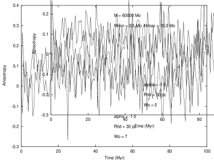
Figure 10: Evolution of the anisotropy for 40% and 99% Lagrangian radii for model W515.

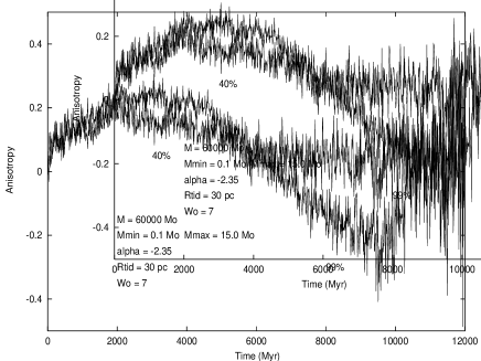
Figure 11: Evolution of the anisotropy for 40% and 99% Lagrangian radii for model W7235.

Figure 12: Evolution of the anisotropy for 10%, 40% and 99% Lagrangian radii for model W735-4 (Family 1).

The anisotropy of the main–sequence stars shows very similar behaviour to that discussed above. Mass segregation forces white dwarfs and neutron stars to occupy the inner parts of the system preferentially. Therefore the anisotropy for them is much more modest than for the main–sequence stars, and stays close to zero. The evolution of the anisotropy agrees qualitatively with the results obtained by Takahashi (1997).

3.4 Mass segregation.

Three main effects may be expected to govern the evolution of the mass function in models of the kind studied in this paper. First, there is a period of violent mass loss due to evolution of the most massive stars. It takes place mainly during the first few hundred million years and its amplitude strongly depends on the slope of the mass function. Secondly, there is the process of rapid mass segregation, caused by two–body distant encounters (relaxation). It takes place mainly during core collapse and, as can be expected, is relatively unaffected by the presence of a tidal field. Thirdly, there is the effect of the tidal field itself, which becomes important after core collapse or even earlier (for models with a shallow mass function and with low concentration). Because the tides preferentially remove stars from the outer parts of the system, which (because of mass segregation) are mainly populated by low–mass stars, one can expect that the mean mass should increase as evolution proceeds, making allowance for stellar evolution.

The basic results are illustrated in Figures 13 to 15 for the total average mass inside the $10\%$ and $50\%$ Lagrangian radii and the tidal radius, and in Figures 16 to 18 for the overall average mass of main–sequence stars and white dwarfs. The violent and strong mass loss due to stellar evolution is characterized by an initial decrease of the average mass. This is best seen in Figure 13 for model W715. The initial average mass in this model is much larger than for other models. It contains a relatively small number of low mass stars and a large number of massive stars. Therefore the evolution of the most massive stars will remove a substantial amount of mass from the system and, consequently, greatly lower the average mass in the whole system. This behaviour is visible (with smaller amplitude) in other models (with steeper mass function) as well, but with one exception. The average mass inside the $10\%$ Lagrangian radius is increasing instead of decreasing (see Figures 14 and 15). For these models, there is enough time for mass segregation to force the most massive stars (in this situation less massive main–sequence stars, neutron stars and massive white dwarfs) to sink into the center and increase the average mass there.

Family 1 models show a much stronger initial decrease of the average mass than the standard models. This is connected with the fact that they contain a much larger number of massive stars than the standard models. The initial mass segregation is only visible for model W735-4 for the 10% Lagrangian radius.

For the standard models with $\alpha=-2.35$ and $-3.5$, mass segregation substantially slows down in the inner parts of the system after the core collapse. This is in good agreement with results obtained by Giersz & Heggie (1997) for small $N$-body simulations, but the reason for that behaviour is still unclear. During the post–collapse phase, for systems with a steeper mass function, mass segregation proceeds further, but at a smaller rate. The effect of tides manifests itself by a gradual increase of the average mass. This increase, as expected, is fastest in the halo and slowest in the core. There is one exception to this rule models which are disrupted before core collapse show a nearly constant rate of increase of the average mass inside the whole system (see Figures 13 and 14). This is probably connected with the fact, that for these disrupting systems stars are removed from the whole body of the cluster.

Family 1 models which enter the long post–collapse evolution phase show a steady, slow decrease of the average mass in the whole system. The total initial average mass for these models is much larger than for the standard models, and therefore stellar evolution is important for a longer time and is competitive with tidal stripping.

Figure 13: Evolution of the average mass inside 10%, 40% Lagrangian radii and $r_{tid}$ for model W715.

Figure 14: Evolution of the average mass inside 10%, 40% Lagrangian radii and $r_{tid}$ for models W3235, W5235 and W7235.

Figure 15: Evolution of the average mass inside 10%, 40% Lagrangian radii and $r_{tid}$ for models W335, W535 and W735.

The evolution of the overall average mass for main–sequence stars and white dwarfs in the standard models shows basically the same features as discussed above (see Figures 16 to 18). When less and less massive main–sequence stars finish their evolution as less and less massive white dwarfs, the average mass of white dwarfs decreases with time. It seems, that in nearly the whole first Gyr the rate of decrease of white dwarf average mass is practically independent of the central concentration and the initial mass function. The differences start to build up later and become most evident close to the collapse time. This can be explained by the fact that models with a steeper mass function contain a smaller number of very massive main–sequence stars. Therefore the total mass of white dwarfs is smaller for these models than for models with a shallower mass function. When less and less massive main–sequence stars finish their evolution, the newly created less massive white dwarfs affect the average mass of white dwarfs more strongly for the steeper mass function than for the shallower one. At the time around core bounce the average mass of white dwarfs increases, particularly for low concentration models with a shallow mass function. Binaries start to be created mainly from the most massive stars (neutron stars and white dwarfs) deep in the core. In interacting with field stars these binaries remove them from the system – preferentially less massive white dwarfs. At the time of core bounce less concentrated models with a shallower mass function are on the verge of disruption. They contain only a small number of stars, and therefore removal of some low mass white dwarfs can lead to substantial changes of the average mass.

For models which enter post–collapse evolution the average mass of main–sequence stars behaves as expected. There is a small initial decrease of the average mass, connected with stellar evolution of the most massive stars. Then there is a period of the gradual increase of the average mass due to tidal stripping and the preferential removal of the least massive stars. At late phases of cluster evolution the increase of average mass speeds up. A different behaviour of the average mass of main–sequence stars is observed for clusters which are disrupted just before core collapse (W515 and W715). For these models removal of low mass main–sequence stars is so strong (because of violent mass loss due to stellar evolution of the most massive stars and induced tidal stripping) that the average mass increases slightly (see Figure 17 and 18). Then the average mass quickly decreases because of stellar evolution and nearly homologous mass removal from the system – most stars are on radial orbits (see Figures 12 and 13).

Generally, Family 1 models show the same features as discussed above. Only for models which enter the long post–collapse evolution phase does the average main–sequence mass decrease slightly instead of increasing. This is in agreement with the evolution of the total average mass for Family 1 models discussed above.

Figure 16: Evolution of the average mass for 10% Lagrangian radius for models W3235, W335; $ms$ and $wd$ means mean–sequence stars and white dwarfs, respectively.

Figure 17: Evolution of the average mass for 10% Lagrangian radius for models w515, W5235 and W535; $ms$ and $wd$ means mean–sequence stars and white dwarfs, respectively.

Figure 18: Evolution of the average mass for 10% Lagrangian radius for models w715, W7235 and W735; $ms$ and $wd$ means mean–sequence stars and white dwarfs, respectively.

4 CONCLUSIONS.

This paper is continuation of Paper I, in which it was shown that the Monte Carlo method is a robust scheme to study, in an effective way, the evolution of a large $N$–body systems. The Monte Carlo method describes in a proper way the graininess of the gravitational field and the stochasticity of the real $N$–body systems. It provides, in almost as much detail as $N$–body simulations, information about the movement of any object in the system. In that respect the Monte Carlo scheme can be regarded as a method which lies between direct $N$–body and Fokker–Planck models and combines most advantages of both these methods. The code has been extended to include stellar evolution, multi–component systems described by a power–law mass function, the tidal field of a parent galaxy and generation of energy by binary–binary interactions. This is the first major step in the direction of simulating the evolution of a real globular cluster.

A small survey (similar to these presented by CW, AH, TPZ and JNR) on the evolution of globular clusters in the Galactic tidal field was carried out. It was shown that the results obtained are in qualitative agreement with these presented by CW, AH, TPZ and JNR. Particularly good agreement is obtained with AH’s $N$-body simulations. JNR’s Monte Carlo results, mainly for strongly concentrated models, disagree with the other models. The Monte Carlo scheme discussed in this paper has some problems with low concentration models and these with a flat mass function. It seems that the collapse times for these models are too short, in comparison with the results of the other methods. However, these models are problematic for all methods; for example, the $N$–body method has problems with proper time scaling. All standard models, for which mass loss due to violent stellar evolution of the most massive stars does not induce quick cluster disruption, evolve in a very similar way. The rate of mass loss, the evolution of the central potential, and the evolution of the average mass, do not depend much on the central concentration of the system. They depend strongly on the index of the mass function. Models of Family 1, on the contrary, show dependence on the initial concentration, as well. The very high initial mass loss across the tidal boundary, connected with the evolution of the most massive stars (for models of Family 1, there are more massive stars than for standard models) forces to substantial changes in the structure of the system and in consequence different evolution of the total mass, anisotropy, etc. Models which are quickly disrupted show only small signs of mass segregation. Models with larger central concentration survive the phase of rapid mass loss and then undergo core collapse and subsequent post–collapse expansion in a manner similar to isolated models. The expansion phase is eventually reversed when tidal limitation becomes important. As in isolated models, mass segregation substantially slows down by the end of core collapse. After core bounce there is a substantial increase in the mean mass in the middle and outer parts of the system, caused by the preferential escape of stars of low mass and by tidal effects. Standard models, which are not quickly disrupted, show a modest initial build up of anisotropy in the outer parts of the system. As tidal stripping exposes the inner parts of the system, the anisotropy gradually decreases and eventually becomes slightly negative. The central part of the system stays nearly isotropic. From the very beginning models of Family 1 develop a modest negative anisotropy in the outer parts of the system. It stays negative until the time of cluster disruption, when it becomes slightly positive (during cluster disruption most stars are on radial orbits).

In order to perform simulations of real globular clusters several additional physical effects have to be included into the code. The tidal shock heating of the cluster due to passages through the Galactic disk, interaction with the bulge, shock–induced relaxation, primordial binaries, physical collisions between single stars and binaries are some of them. Inclusion of all these processes does not pose a fundamental theoretical or technical challenge. It will allow us to perform detailed comparison between simulations and the observed properties of globular clusters, and will also help to understand the conditions of globular cluster formation and explain how peculiar objects observed in clusters can be formed. These kinds of simulations will also help us to introduce, in a proper way, into future $N$–body simulations all the necessary processes required to simulate evolution of real globular clusters on a star–by–star basis from their birth to their death.

Acknowledgments I would like to thank Douglas C. Heggie and Rainer Spurzem for stimulating discussions, comments and suggestions. I also thank DCH for making the $N$–body results of standard model simulations available. This work was partly supported by the Polish National Committee for Scientific Research under grant 2–P03D–022–12.

References

- [1] Aarseth S.L., 1985, in Brackbill J.U., Cohen B.,I., eds, Multiple Time Scales. Academic Press, New York, p.377
- [2] Aarseth S.L., 1999a, Cel. Mech. Dyn. Astr., 73, 127
- [3] Aarseth S.L., 1999b, PASP, 111, 1333
- [4] Aarseth S.L. & Heggie D.C., 1998, (AH), MNRAS, 297, 794
- [5] Baumgardt H., 2000, in Star 2000, Dynamics of Star Clusters and the Milky Way
- [6] Chernoff D.F. & Weinberg M.D., 1990, (CW), ApJ, 351, 121
- [7] Djorgovski S.G. & Meylan G., eds., 1993, Structure and Dynamics of Globular Clusters. A.S.P., San Francisco
- [8] Einsel Ch., Spurzem R., 1999, MNRAS, 302, 81
- [9] Gao B., Goodman J., Murphy B., Cohn H., 1991, ApJ, 370, 567
- [10] Giersz M., 1998, (Paper I), MNRAS, 298, 1239
- [11] Giersz M., 2000, in Dynamics of Star Clusters and the Milky Way, ASP Conference Series, eds S.Deiters, B. Fuchs, A. Just, R. Spurzem and R. Wielen (astro-ph/0006438)
- [12] Giersz M. & Heggie D.C., 1994, MNRAS, 270, 298
- [13] Giersz M. & Heggie D.C., 1996, MNRAS, 279, 1037
- [14] Giersz M. & Heggie D.C., 1997, MNRAS, 286, 709
- [15] Giersz M. & Spurzem R., 2000, MNRAS, accepted (astro-ph/9911504)
- [16] Gnedin O.Y., Lee H.M. & Ostriker J.P., 1999, ApJ, 552, 935
- [17] Heggie D.C., 1975, MNRAS, 173, 729
- [18] Heggie D.C., 2000, private information
- [19] Heggie D.C. & Mathieu R.M., 1986, in Hut P., McMillan S.L.W., eds., The Use of Supercomputers in Stellar Dynamics., Springer Berlin, 233
- [20] Heggie D.C., Hut P. & McMillan S.L.W., 1996, ApJ, 467, 359
- [21] Heggie D.C., Giersz M., Spurzem R., Takakashi K., 1999, in Highlights of Astronomy, vol 11, ed. J. Andersen, 591
- [22] Hénon M., 1971, Astrophys. Sp. Sci., 14, 151
- [23] Hénon M., 1975, in Hayli A., ed., Dynamics of Stellar Systems, Reidel: Dordrecht, 133
- [24] Hut p., McMillan S.L.W., Goodman J., Mateo M., Phinney E.S., Pryor C., Richer H.B, Verbunt F. & Weinberg M., 1992, PASP, 104, 981
- [25] Hut P. & Makino J., eds. 1996, Dynamical Evolution of Star Clusters. A.S.P., San Francisco
- [26] Janes K., ed. 1991, The Formation and Evolution of Star Clusters. A.S.P., San Francisco
- [27] Joshi K.,J., Nave C. & Rasio F.A., 1999a, ApJ submitted (astro-ph/9912155)
- [28] Joshi K.,J., Rasio F.A. & Portegies Zwart S., 1999b, (JNR), ApJ submitted (astro-ph/9909115)
- [29] Kroupa P, Tout C.A. & Gilmore G., 1990, MNRAS, 244, 76
- [30] Makino J., 1989, in Dynamics of Dense Stellar Systems, ed. D. Merritt (Cambridge: Cambridge Univ. Press), 201
- [31] Makino J., Taiji M., Ebisuzaki T. & Sugimoto D., 1997, ApJ, 480, 432
- [32] Makino J., 1996b ApJ, 471, 796
- [33] Makino J., Tanekusa J. & Sugimoto D., 1986, PASJ, 38, 865
- [34] Marchant A.B, & Shapiro S.L., 1980, ApJ, 239, 685
- [35] Meylan G., & Heggie D.C., 1997 in The Astronomy and Astrophysics Review, 8, 1
- [36] Mikkola S., 1983, MNRAS, 205, 733
- [37] Mikkola S., 1984, MNRAS, 208, 75
- [38] Portegies Zwart S.F. & Verbunt F., 1996, A&A, 309, 179
- [39] Portegies Zwart S.F., Hut P., Makino J. & McMillan S.L.W., 1998, A&A, 337, 363
- [40] Rauch K.P., & Tremaine S., 1996, New Astronomy, 1, 149
- [41] Smith G.H & Brodie J.P, eds., 1993 The Globular Cluster–Galaxy Connection. A.S.P, San Francisco
- [42] Spitzer L., Jr., 1975, in Hayli A., ed, Dynamics of Stellar Systems, Reidel: Dordrecht, p.3
- [43] Rubenstein E.P. & Bailyn C.D., 1997, ApJ, 474, 701
- [44] Spitzer L., Jr., 1987, Dynamical Evolution of Globular Clusters. Princeton Univ. Press, Princeton, 77
- [45] Spurzem R., 1994, in Ergodic Concepts in Stellar Dynamics, eds. D. Pfenniger & V.G. Gurzadyan (Springer–Vlg., Berlin, Heidelberg), 170
- [46] Spurzem R. & Aarseth S.J., 1996, MNRAS, 282, 19
- [47] Spurzem R. & Giersz M., 1996, MNRAS, 283, 805
- [48] Stodółkiewicz J.S., 1982, Acta Astr., 32, 63
- [49] Stodółkiewicz J.S., 1986, Acta Astr., 36, 19
- [50] Takahashi K., 1995, PASJ, 47, 561
- [51] Takahashi K., 1996, PASJ, 48, 691
- [52] Takahashi K., 1995, PASJ, 49, 547
- [53] Takahashi K. & Lee H.M., 1999, MNRAS submitted (astro-ph/9909006)
- [54] Takahashi K., & Portegies Zwart, S.F., 1998, ApJ, 503, L49
- [55] Takahashi K., & Portegies Zwart, S. F., 1999, (TPZ), ApJ submitted (astro-ph/9903366)
- [56] Tout C.A, Aarseth S.J., Pols O.R. & Eggleton P.P, 1997, MNRAS, 291, 732