A Model of Void Formation

Abstract

We introduce a simple model for the formation of voids. In this model the underdensity of galaxies in voids is the product of two factors. The first arises from a gravitational expansion of the negative density perturbation. The second is due to biasing: galaxies are less likely to form in an underdense region. One feature of the model is an upper cutoff in void sizes. We calculate the volume filling factor of characteristic voids for different CDM models and find that our formation model points to $\Lambda$CDM models as preferred models of the power spectrum. A natural consequence of our model is that the underdensity of the dark matter inside voids is smaller than the galaxy underdensity.

1 Introduction

Visual inspection of redshift surveys has revealed (De Lapparent et al., 1986; Kirshner et al., 1987; Geller and Huchra, 1989; Da Costa et al., 1995; Geller et al., 1997; Shectman et al., 1996) that a large fraction of the universe is made of ”voids”: regions in which the typical galaxy density is significantly lower than the mean galaxy density. Most galaxies tend to be found in two dimensional sheets that encompass these voids. Using the “VOID FINDER” algorithm, an automated algorithm that detects voids in three dimensional surveys and measures their volume, El-Ad and Piran determined the sizes and depths of voids in several surveys: SSRS2, IRAS and ORS (El-Ad and Piran, 1997; El-Ad et al., 1997; El-Ad and Piran, 1999). They found that the void distribution is remarkably stable and that different surveys that encompass the same regions in the sky see the same voids. They also found that: (i) The voids occupy $\approx 50\%$ of the volume. (ii) Void radii are in the range 13-30$h^{-1}$ Mpc. There appears to be an upper cutoff to the sizes of the voids. This upper limit does not depend on the properties of a particular survey or on the effective depth. This upper cutoff is also seen in visual inspection of the deepest survey existing today, the LCRS (Shectman et al., 1996), whose effective depth is 100$h^{-1}$ Mpc. (iii) The density contrast of galaxies in voids is in the range $[-0.70,-0.95]$.

In current surveys the sizes of observed structures are not much smaller than the effective depth of the survey. Therefore only about a dozen voids have been identified so far. Hence, there is not enough data to produce a good statistics on the distribution of the voids’ sizes and depths. This situation will change with the new generation of automated redshift surveys - the 2dF (Lahav, 1996) and the SDSS (Loveday, 1996). With these surveys we will be able to identify dozens of voids and to quantify their features. With this situation in mind we are beginning to set here the ground for the analysis of these properties and for a comparison of the observations with a simple model for void formation.

The existence of significant inhomogeneities on the scale of tens of Mpc should be an important clue as to the formation of large scale structure, and can be useful in exploring the power spectrum on this scale range. Indeed positive fluctuations on scales of 10 Mpc (clusters and super clusters) provide a powerful tool to explore the power spectrum (see Bahcall and Fan (1998)). However voids have not been used as yet. This is due to several reasons. The present day sky surveys are not comprehensive enough to allow a full quantitative assessment of void sizes and of the distribution function of void sizes. Secondly, there is a lack of a simple theory for the formation of voids.

A theory for the formation of voids should explain the physical mechanisms which operate in the formation of the voids. It should be able to explain qualitatively the appearance of the apparent upper cutoff on their sizes. Using this theory one could compare the properties of voids (more specifically, voids sizes and filling factor) that arise from different primordial perturbation spectra with the observations. Another goal of such a model is to predict the underdensity of the dark matter within the voids and to provide us with a prediction of the effective biasing factor within the voids.

Blumenthal et al. (1992), Dubinski et al. (1993) and Piran (1997) considered a purely gravitational scenario for the formation of voids. Their model is based on the assumption that light traces matter on the scale of voids. In this case the observed underdensity in the galaxy distribution corresponds to a comparable underdensity in the dark matter. According to this model the observed voids today are primordial negative perturbations that grew gravitationally and reached shell crossing today. Shell crossing happens when the radius of the perturbation has grown by a factor of 1.7, corresponding to a density contrast of -0.8. However, at this stage the perturbation is highly non linear (the corresponding linear amplitude would have been 2.7). Such a large amplitude requires too much power on the scale of voids and it is inconsistent with the number density of clusters and super-clusters on slightly lower scales.

In this paper we suggest a new approach that may be used as a formalism for analyzing voids. We present a simple intuitive model which describes the formation of voids as due to gravitational growth and biasing. We relax the assumption that light traces matter on these large scales and claim that the observed underdensity in the galaxy density is a product of two factors. The first arises from a simple gravitational expansion of the negative density perturbation. The second factor arises due to biasing: galaxies are less likely to form in an underdense region. We consider spherical underdensities. This is, quite generally, a good approximation as negative density perturbations become more and more spherical as they evolve (Icke (1984), Lin et al. (1965)). To estimate the biasing factor we use a simple peak biasing formalism which was developed by David and Blumenthal (1992) for the calculation of biasing in clusters.

Our model explains why voids appear in a relatively small range of sizes and in particular why there is an upper limit to the sizes of the voids. We use it to calculate the expected sizes and volume filling factor of voids in different cosmological models and we compare our results with current observations. The comparison is made to a simple interpretation of the data - voids occupy 50% of the volume, their radii are in the range of 13-30$h^{-1}$ Mpc and the typical underdensity in the galaxy distribution is taken to be -0.8. This is a simplified picture and should be modified in the future when data from new surveys is available and when we have a more refined model. Finally we use our model to calculate the expected dark matter underdensity within the voids.

We find that cosmological models which agree with other constraints on the power spectrum can in general produce the observed voids even if not as many as observed. In particular we find, in-spite of the crudeness of the model and the uncertainties in present day data, that flat $\Lambda$CDM with a current density parameter $0.25<\Omega_{0}<0.35$ is the most preferable model, in agreement with other observations.

The paper is organized as follows. In section (2) we present the details of the model and a general calculation of the underdensity of galaxies inside voids. In section (3) we calculate the relative volume of the universe in the form of voids in universes characterized by different cosmological parameters and CDM power spectra. We discuss the implication of our results in section (4).

2 The Model

We begin by calculating the dynamics of a negative density perturbation in a general cosmology. Our goal is to calculate $\eta$, the ratio of the comoving size of the perturbation to its initial comoving size, in terms of $\delta_{L}$, the linear amplitude of the perturbation. The factor $\eta^{-3}-1$ is the underdensity due to the gravitational growth. As it is expressed in terms of $\delta_{L}$ it can be calculated directly from the linear power spectrum once the relevant scale is chosen. Then we turn to calculate the underdensity of galaxies in a larger scale negative density perturbation.

2.1 Gravitational Growth of Voids

During the linear phase perturbations grow in amplitude but not in comoving size. As the perturbations become nonlinear their comoving radius begins to grow. To find $\eta$ we solve the differential equation that governs the evolution of a spherical shell surrounding a negative density region. At some initial time, $t_{i}$ (at a redshift $z_{i}$), the shell is expanding at the same rate as the background (that is we have an initial density perturbation). The initial small (negative) density contrast is $\delta_{i}$ and the initial radius of the shell is $R_{i}$. The background evolution is characterized by the present values of the Hubble constant $H_{0}$, the density parameter $\Omega_{0}$, and the cosmological constant $\Lambda$. For convenience we define: $\lambda_{0}=\Lambda/3H_{0}^{2}$. As long as there is no shell crossing the mass inside the shell remains constant and energy conservation yields a differential equation for $R$, the shell’s radius (Lahav et al., 1991):

$${\dot{R}}^{2}= H_{0}^{2}[-\Omega_{0}(1+z_{i})^{3}R_{i}^{2}\delta_{i}-(\Omega_{0}+\lambda_{0}-1)(1+z_{i})^{2}R_{i}^{2}+$$

$$\Omega_{0}(1+z_{i})^{3}R_{i}^{3}(1+\delta_{i})/R+\lambda_{0}R^{2}].$$

We combine this equation with the equation for the background’s redshift:

$$\frac{1}{1+z}\frac{d(1+z)}{dt}=-H_{0}P(z)$$ (2)

where

$$P(z)=\Omega_{0}(1+z)^{3}-(\Omega_{0}+\lambda_{0}-1)(1+z)^{2}+\lambda_{0}$$ (3)

to obtain an equation for $dR/dz$. We solve this equation numerically and obtain the radius $R$ as a function of the redshift. Since the comoving radius increases as $1/(1+z)$ we find that $\eta=[R(z)(1+z)]/[R_{i}(1+z_{i})]$.

The growing solution of the linear perturbation equation is given by Heath (1977):

$$\delta_{L}^{+}=CP^{1/2}(z)\int_{z}^{\infty}\frac{(u+1)du}{P(u)^{3/2}}.$$ (4)

The constant C depends on the initial conditions. Since we have considered earlier an initial density perturbation, $\delta_{i}$, the corresponding initial density contrast of the growing mode is $3\delta_{i}/5$.

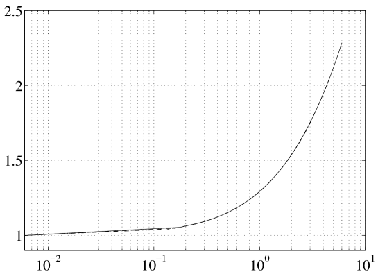
Figure 1: The growth factor, $\eta$, of a spherical perturbation as a function of the corresponding linear amplitude for three cases: an $\Omega_{0}<1$ open universe, $\Omega_{0}+\lambda_{0}=1$ and a flat universe with $\lambda_{0}=0$.

We can now obtain the growth factor as a function of $\delta_{L}$ (we will drop the ⁺ from now on). Fig. (1) depicts $\eta$ as a function of $\delta_{L}$ for three cases: an Einstein-de Sitter universe ($\Omega_{0}=1$, $h=0.5$, $\lambda_{0}=0$), an open low density universe without a cosmological constant ($\Omega_{0}=0.37$, $\lambda_{0}=0$) and a flat low density model, with cosmological constant ($\Omega_{0}=0.37$, $\lambda_{0}=0.63$). The function $\eta(\delta_{L})$ is practically independent of the cosmological parameters and the different curves overlap each other. For very small values of $\delta_{L}$, when the perturbations are still linear, the growth factor $\eta$ is very close to 1. This is expected since in the linear theory perturbations grow in amplitude only. $\eta$ increases only as the perturbation becomes non linear.

2.2 Biased Galaxy Formation in Voids

We turn now to the statistical determination of the underdensity of galaxies within voids. Following David and Blumenthal (1992) we consider a simple model in which galaxies form in peaks that exceed a global galaxy formation threshold. We define the “efficiency” of galaxy formation in some volume $V$, $\epsilon^{V}$, as the fractional volume of $V$ which is contained in galaxies:

$$\epsilon^{V}=\frac{V_{gal}}{V_{tot}}$$ (5)

To determine $\epsilon^{V}$ we use the conditional probability $f(\nu_{g},\nu_{v})$ of finding a galaxy-size fluctuation with a relative over-density $\nu_{g}=\frac{\delta_{g}}{\sigma_{g}}$ within a void size fluctuation with a relative under-density $\nu_{v}=\frac{\delta_{v}}{\sigma_{v}}$. Here $\sigma_{g}$ and $\sigma_{v}$ are the rms mass fluctuations filtered on galaxy and void scales, respectively. The scale of a galaxy, $R_{g}$ is related to its mass $M_{g}$ (including the dark matter) through $M_{g}=(4\pi/3)R_{g}^{3}<\rho>$.

$$f(\nu_{g},\nu_{v})=\frac{1}{2\pi\sqrt{1-r^{2}}}\exp[-\frac{1}{2\sqrt{1-r^{2}}}(\nu_{g}^{2}+\nu_{v}^{2}+2r\nu_{g}\nu_{v})].$$ (6)

$r$ is the correlation coefficient between the two scales, given by $\sigma_{gv}^{2}/\sigma_{g}\sigma_{v}$, where:

$$\sigma_{gv}^{2}=\frac{1}{(2\pi)^{3}}\int d^{3}\mathbf{k}\left|\delta_{\mathbf{k}}\right|^{2}W(kR_{g})W(kR_{v}),$$ (7)

and $W(kR)$ is a window function. We choose a top-hat window function:

$$W(kR)=\frac{3(\sin{kR}-kR\cos{kR})}{(kR)^{3}}$$ (8)

We use a single typical galaxy mass of $M_{g}=1.2\cdot 10^{12}M_{\odot}\frac{(M/L)}{100M_{\odot}/L_{\odot}}$ which is the median of the galaxy luminosity function. This is clearly an approximation and possibly the crudest one we make in this work. The scale related to this mass, $R_{g}$, varies according to the cosmological parameters of the model. Assuming that only the peaks that exceed a global threshold $\nu_{th}$ become luminous galaxies the efficiency of galaxy formation in voids of a given radius $R$ and with a given $\nu_{v}$ is:

$$\epsilon^{void}(\nu_{v},R)=\frac{\int_{\nu_{th}}^{\infty}f(\nu_{g},\nu_{v})d\nu_{g}}{\int_{-\infty}^{\infty}f(\nu_{g},\nu_{v})d\nu_{g}}=\frac{1}{2}{\rm erfc}\left[\frac{\nu_{th}+r\nu_{v}}{\sqrt{2(1-r^{2})}}\right].$$ (9)

The galaxy formation threshold, $\nu_{th}$, is calculated using the global efficiency of galaxy formation:

$$\epsilon^{bg}=\epsilon^{void}(R_{v}=\infty)=\frac{1}{2}{\rm erfc}\frac{\nu_{th}}{\sqrt{2}}$$ (10)

Empirically, one possible way of determining the fraction of mass residing in galaxies is to divide the mass-to-light ratio of a typical galaxy by the mass-to-light ratio of the universe. Following Bahcall et al. (1995) we take the M/L ratio of the universe to be 1350$\Omega_{0}$h and that of a typical galaxy to be 100h. Now we have

$$\frac{1}{2}{\rm erfc}\frac{\nu_{th}}{\sqrt{2}}=\frac{(M/L)_{gal}}{1350\Omega_{0}h}$$ (11)

Using eq. 11 we can determine, for any given $\Omega_{0}$, the global galaxy formation threshold.

2.3 The combined underdensity

The current underdensity of galaxies in voids, $\delta_{gal}$, is

$$1+\delta_{gal}=\frac{\rho_{gal}^{void}}{\rho_{gal}^{bg}}=\frac{\epsilon^{void}}{\epsilon^{bg}\eta^{3}}$$ (12)

where $\rho_{gal}^{void}$ is the density of galaxies in the void and $\rho_{gal}^{bg}$ is their average density in the background universe. The second equality holds once the growth factor of the void is taken into account and all the galaxies are taken to be of the same typical scale ($\approx 1h^{-1}$Mpc).

3 The Void Content of the Universe in Different CDM Models

Given the model described above we shall now calculate the expected sizes and the volume filling factors of voids in different cosmological models. We also calculate the dark matter underdensity in voids in these models. Our aim is to find the dependency of the filling factor on cosmological parameters. A second goal is to predict the dark matter underdensity in voids and through this to learn of the biasing between dark and luminous matter on these large scales.

We consider first the SCDM model ($\Omega_{0}=1$, $h_{0}=0.5$, $\Lambda=0$, $n=1$, $\Omega_{b}=0.0125h^{-2}$). It is already established that this is not a valid model of the universe; it does not agree simultaneously with COBE and with cluster abundance data. However because of the simplicity of the SCDM model we use it as a tool to demonstrate how the void content of the universe changes with the normalization of the power spectrum. We use the transfer function calculated by Bardeen et al. (1986) as the shape of the dark matter power spectrum. For the normalization we consider two possibilities: COBE normalization as calculated by Bunn and White (1997) ($\sigma_{8}=1.27$) and cluster abundance normalization as given by Pen (1998) ($\sigma_{8}=0.53$).

We present contour lines of constant galaxy underdensity as a function of the radius of the voids today $R$ and the relative underdensity in the dark matter $\nu$. Figure [2] depicts several contour lines for the cluster normalized SCDM model. If we look at constant $\nu$ we find that there are relatively more galaxies in larger voids. This is due in part to the statistical properties of the fluctuations and in part to the gravitational expansion of the underdensities. At larger scales the amplitude of the perturbations is smaller, so to form a galaxy in a larger underdensity we need galaxy size perturbations of smaller amplitude. These will be more abundant because the distribution function of the fluctuations is a Gaussian. Thus there will be more galaxies in larger voids and the relative underdensity of the galaxies will decrease. The gravitational expansion factor does not compensate for this - in fact, it becomes less important because $\delta_{L}$ of the underdensities decreases as $R$grows (see Fig[1]). If we look at voids of constant radius we see that there are relatively less galaxies at larger $\nu$. The contribution to this behavior is also two-fold. Negative perturbations of higher $\nu$ correspond to deeper voids; In such voids we need galaxy size perturbations of larger amplitude to form galaxies. These are less abundant and therefore the relative underdensity of the galaxies is larger in deeper voids. To this we add the fact that negative perturbations of higher $\nu$ are of higher $\delta_{L}$ and for these the gravitational factor is bigger. Thus the volume of the void will grow and the relative underdensity in the galaxy distribution will be even greater.

An important feature to notice in this figure is that for a given underdensity of the galaxy distribution inside a void, larger voids are produced exponentially more rarely as they require large and hence extremely rare initial perturbations. Thus there is a sharp upper limit to the sizes of voids.

To compare with observations we calculate the filling factor of the voids. We calculate the fraction of the universe which is composed of spherical and isolated negative density perturbations that are large enough and deep enough to produce voids of radii 13-30 $h^{-1}$Mpc. The number of spherical inhomogeneities of a radius R and an amplitude in the range [$\delta,\delta+d\delta$] inside the horizon is:

$$N(R,\delta)d\delta=\frac{c^{3}H_{0}^{-3}}{R^{3}}\cdot\frac{1}{(2\pi\sigma_{R}^{2})^{1/2}}e^{-\delta^{2}/2\sigma_{R}^{2}}d\delta.$$ (13)

Clearly the isolated spherical approximation would break down at low $\nu$ values and it might be violated around the lower limits ($\nu\sim 1.5$) of our integration. We expect it to hold at higher values. The total volume of the corresponding voids is $(\eta R)^{3}\cdot N(R,\delta)$ and the relative volume is

$$f(R,\delta)d\delta=\frac{\eta^{3}}{(2\pi\sigma_{R}^{2})^{1/2}}\cdot e^{-\delta^{2}/2\sigma_{R}^{2}}d\delta$$ (14)

The voids with radii 13-30 $h^{-1}$Mpc correspond to initial fluctuations of sizes of about 10-25$h^{-1}$Mpc, depending on the model. Thus to obtain the overall filling factor, denoted by $f$, we integrate equation (14) along the contour of $\delta_{gal}=-0.8$ in the appropriate range. This method of counting might be complicated by the possibility of over-counting: a void of certain radius and amplitude might be counted again as a void of larger radius and smaller amplitude. This cannot happen if the underdensity $\delta$ increases with R, as the larger void would be deeper. We therefore checked the behavior of $\delta$, and found that it increases monotonically with R.

We have carried out this calculation for two CDM models with different normalizations. The contour lines of $\delta_{gal}=-0.8$ of the two models are presented in Fig. [3]. The difference between the two models is very pronounced: the model with more power on the scale of the voids (COBE normalized) yields more voids. This can be explained as follows: when the power on the scale of the voids is larger, the amplitude needed to produce the voids that we see today is reached by fluctuations with lower $\nu$ which are therefore more frequent. In models with less power on void scales, the same amplitude of underdensities requires higher $\nu$ values and are therefore less frequent. This is reflected in the calculated values of the filling factors $f=33\%$ for the COBE normalized model, and only 11% for the cluster normalized model.

However, neither of these CDM models is an acceptable model of the universe. We estimate now the void content of the universe in the context of power spectra which are compatible with observations. We consider Open CDM and flat $\Lambda$CDM models. The transfer function used is, as above, (Bardeen et al., 1986). The normalization will be according to the 4-year COBE DMR experiment, as calculated by Bunn and White (1997). To determine the models’ parameters we first set $\Omega_{0}$, then we choose a tilt such that the model is also cluster normalized. This is done by calculating $\sigma_{8}$ and finding a tilt such that the normalization condition given by Pen (1998):

$$\sigma_{8}=(0.53\pm 0.05)\Omega_{0}^{-0.45}$$ (15)

for open models and

$$\sigma_{8}=(0.53\pm 0.05)\Omega_{0}^{-0.53}$$ (16)

for flat models is satisfied. We take Hubble’s constant to be $H_{0}=65$ $Kmsec^{-1}Mpc^{-1}$ in agreement with recent results from HST Key project ($H_{0}=0.71\pm 0.06$, see Mould et al. (2000)) and measurements of time delay between multiple images of gravitational lens systems ($H_{0}=0.69^{+13}_{-19}$, see Biggs, et al. (1999)). $\Omega_{b}h^{-2}=0.015$ in all models. The models are described in Table 1. The first two columns of the table give $\Omega_{0}$ and $n$. In the third column we list $\sigma_{8}$, the amplitude of mass fluctuations in spheres of radius 8$h^{-1}$Mpc. All $\sigma_{8}$ are within the ranges allowed by the cluster normalisation. As another check for the validity of our models, we show that the shape parameter $\Gamma$ of each of the models is within limits ($0.15<\Gamma<0.3$) allowed by measurments of the angular correlation function from the APM galaxy survey (Efstathiou, Bond and White, 1992). The values of $\Gamma$ are listed in the fourth column. Finally the fifth column gives the calculated filling factor and in the sixth column the calculated dark matter underdensity is listed.

As before, we present the results as contour lines of constant $\delta_{gal}$ as a function of the radius of the voids today, $R$, and as a function of their relative underdensity in the dark matter, $\nu$. The contour lines for the Open and $\Lambda$ CDM models are presented in figures [4,5] respectively. We notice, first, that all the models show a common behaviour which was manifested also in the SCDM models: Larger voids of $\delta_{gal}=-0.8$ are produced exponentially more rarely. The sharp upper limit to the sizes of voids exists in all CDM models.

		$\Omega_{0}$	n	$\sigma_{8}$	$\Gamma$	$f(\%)$	$\delta_{DM}$
1	Open-	0.3	1.3	0.92	0.18	19	-0.56
2	CDM	0.35	1.17	0.85	0.21	18	-0.53
3		0.4	1.07	0.81	0.24	18	-0.52
4		0.45	0.98	0.76	0.27	18	-0.49
5	$\Lambda$CDM	0.2	1.2	1.2	0.11	31	-0.60
6	(flat)	0.25	1.1	1.11	0.15	29	-0.56
7		0.3	1	0.95	0.18	25	-0.53
8		0.35	0.96	0.93	0.21	25	-0.52
9		0.4	0.91	0.86	0.24	24	-0.50
10		0.45	0.88	0.83	0.27	22	-0.49

Table 1: A list of the models considered.

Figure [4] describes voids of $\delta_{gal}=-0.8$ in Open CDM models. It is clear that the void distribution does not depend strongly on $\Omega_{0}$. The filling factor is almost constant, having values 18-19%. Figure [5] describes the same voids in flat $\Lambda$CDM models. Here there is a stronger dependence of the void distribution function on $\Omega_{0}$, and the filling factor is larger than in the open models. It is in the range 22-31%, decreasing with $\Omega_{0}$.

We have also calculated the expected underdensity of the dark matter. This underdensity is given simply by $\delta_{DM}=\eta^{-3}-1$. It is listed, for 20 $h^{-1}$Mpc voids in the different models, on sixth coloumn of table [1]. The underdensities are in the range [-0.5,-0.6] for all the models. These typical values are a factor of 1.3-1.6 smaller than the galaxy underdesity, indicating this factor as the biasing between galaxies and dark matter perturbations on the $20h^{-1}$Mpc scale within the voids.

4 Discussion

We have presented here a model for the formation of voids. In this model voids arise from initial negative density perturbations. Such underdensities grow in comoving volume and this growth increases the underdensities of both the galaxies and the dark matter within the voids. The galaxy underdensity is enhanced further since positive galaxy size perturbations are less frequent within negative void size perturbations. This mechanism inhibits the formation of galaxies within the voids. In our model both mechanisms contribute comparable factors to the overall galaxy underdensity.

We use the model to investigate the void content of the universe for different power spectra which are in agreement with COBE and cluster abundance data. Qualitatively we found, in all the cosmological models we tested, that the probability of finding voids of a certain $\delta_{gal}$ falls exponentially with the radius. This behavior may explain the observed upper limit of the radii of voids.

In order to quantitatively test our model, we have calculated the filling factor of the observed voids ($R_{v}\in[13-30]h^{-1}$Mpc, $\delta_{gal}=-0.8$). We find that in all the models that we considered the observed voids fill only half of the expected volume. However, there is a clear trend toward higher filling factors in $\Lambda$CDM models where the relevant voids appear more frequently and fill a larger fraction of the universe. We also found that in the open models that we have tried, since the power spectra were very similar, the distribution of the void sizes and the filling factor did not change with $\Omega_{0}$. However, in $\Lambda$CDM models, as $\Omega_{0}$ grows the relevant voids become less frequent and the void content of the universe decreases. It can be explained by the fact that as we increase $\Omega_{0}$, the amplitude of fluctuations on the scale of voids is decreased. The most preferable models are the $\Lambda$CDM models with $0.25<\Omega_{0}<0.35$: these comply with all the constraints and have the highest void filling factors. Still even these values fall short of the observations by a factor of $\approx 1.4$.

We suspect that the small filling factor is due in part to the oversimplified model of galaxy formation that we have used. A more realistic model should allow for a range of galaxy masses and a more elaborate biasing mechanism between the dark matter and galaxies. This will be the next step towards a more reliable model. Also note that, as already mentioned, another important assumption of our model is that of spherically symmetric isolated evolution. We have assumed that the underdensities are spherical and isolated when calculating the gravitational growth and the filling factor, ignoring possible mergers between neighboring voids and the influence of positive overdensities on nearby underdensities. Void mergers might lead to the disappearance of smaller voids with deeper underdensities alongside with the appearance of larger asymmetric voids. Positive nearby overdensities could exert forces on matter inside underdensities and increase their growth rate. Both effects could increase the filling factor of voids.

Finally we have computed the underdensity of dark matter in typical voids of radius 20$h^{-1}$Mpc. While the dark matter is influenced only by the gravitational expansion of the negative density perturbations the number of galaxies is also influenced by the biasing factor. For this reason we have $\mid\delta_{DM}\mid<\mid\delta_{gal}\mid$. The expected dark matter underdensities that we find are about a factor of 1.3-1.6 lower than the underdensities of the galaxy density. These values should be regarded only as an upper limit to the real underdensity expected in nature. Since real voids are more frequent, they must correspond to lower $\nu$ values and their gravitational growth factor would be smaller. This will result in a less negative dark matter density contrast. This prediction should be compared with estimates of the dark matter density in voids from N-body simulations and with future measurements of the dark matter underdensity within the voids.

It will be interesting to apply our model to account for evolution of void sizes and abundances as a function of redshift. We suspect that in critical density universes the evolution of voids will be stronger than in low density universes: We have shown in section 2 that the growth of the radius of the void depends only on the linear amplitude of the perturbation and not on cosmological parameters. Thus in a universe with $\Omega_{0}=1$ where the linear amplitude grows like the scale factor, the radius of the void will grow constantly. However, in models where matter ceases to dominate, such as open models which become curvature dominated at small z or flat models with a cosmological constant which begins to dominate at late times the linear amplitude reaches a constant value and stops growing. In such cases, the comoving radius of the voids will also stop growing at late times. Thus we could use the model to predict the change in comoving radius of voids as function of z in different cosmological models and by comparing to the next generation of deep sky surveys discriminate between low and critical density models (for example, in critical density universes older voids will be smaller in radius and the galaxy underdensity in them will also be smaller).

Upcoming sky surveys, such as the Sloan Digital Sky Survey, will increase the available galaxy distribution data by several orders of magnitude. In particular such surveys will include more voids and hopefully enough voids to obtain the distribution and evolution of the void sizes. That would allow us to compare our model with observations in a more accurate way and constrain $\Omega_{0}$ and other cosmological parameters using the void distribution.

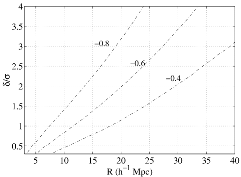
Figure 2: Contours of constant $\delta_{gal}$ are displayed as a function of the radius of the voids today, R, and the relative underdensity of the dark matter, $\nu_{v}$, in a standard CDM model which is cluster-normalised. We can see that the typical voids ($R=20h^{-1}$Mpc $\delta_{gal}=-0.8$) are 3$\sigma$ objects i.e they are produced very rarely.

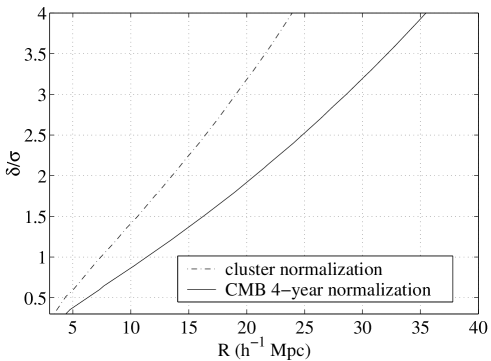
Figure 3: Two contours of $\delta_{gal}=-0.8$ are displayed. One is for cluster abundance normalized SCDM (dashed). The other is for COBE-normalized SCDM. The effect of the different normalizations is very obvious: When the power on the scale of voids is higher (COBE) the observed voids are much more frequent.

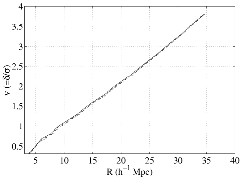
Figure 4: Contours of $\delta_{gal}=-0.8$ in the four Open CDM models we checked are displayed as a function of the radius of the voids today, R, and relative underdensity, $\nu$. It is clear that in open models the distribution of the voids is not a function of $\Omega_{0}$. This can be explained by the fact that the power spectra for these models are almost the same on all scales.

Figure 5: The contours of $\delta_{gal}(\nu,R)=-0.8$ in the six $\Lambda$CDM models as a function of the radius of the voids today, $R$, and of the relative underdensity of the void, $\nu$. Here we see a stronger dependance on $\Omega_{0}$, and also we see that voids are more frequent in these models than in the open models.

References

- Bahcall and Fan (1998) N. A. Bahcall and X. Fan. ApJ, 504:1, 1998.
- Bahcall et al. (1995) N. A. Bahcall, L. M. Lubin, and V. Dorman. ApJ, 447:L81, 1995.
- Bardeen et al. (1986) J. M.Bardeen, J. R.Bond, N. Kaiser and A. S.Szalay. ApJ, 304, 1986.
- Biggs, et al. (1999) A. D. Biggs, I. W. A. Browne, P. Helbig, L. V. E. Koopmans, P. N. Wilkinson, and R. A. Perley MNRAS, 304:349, 1999.
- Blumenthal et al. (1992) G. R. Blumenthal, L. N. Da Costa, D. S. Goldwirth, M. Lecar, and T. Piran. ApJ, 388:234, 1992.
- Bunn and White (1997) E. F.Bunn, and M. White, ApJ 480:6,1997.
- Da Costa et al. (1995) L. Nicolaci Da Costa, M. J. Geller, P. S. Pellegrini, D. W. Latham, A. P. Fairall, R. O. Marzke, C. N. A. Willmer, J. P. Huchra, J. H. Calderon, M. Ramella, and M. J. Kurtz. ApJ, 100:L1, 1995.
- David and Blumenthal (1992) L. P. David and G. R. Blumenthal. ApJ, 389:510, 1992.
- De Lapparent et al. (1986) V. De Lapparent, M. J. Geller, and J. P. Huchra. ApJ, 302:L1, 1986.
- Dekel and Lahav (1999) A. Dekel & O. Lahav, 1999, ApJ, 520, 24
- Dubinski et al. (1993) J. Dubinski, L. N. Da Costa, D. S. Goldwirth, M. Lecar, and T. Piran. ApJ, 410:458, 1993.
- Efstathiou, Bond and White (1992) G. Efstathiou, J. R. Bond and S. D. M. White MNRAS, 258:1P, 1992.
- El-Ad and Piran (1997) H. El-Ad and T. Piran. ApJ, 491:421+, December 1997.
- El-Ad and Piran (1999) H. El-Ad and T. Piran. astro-ph/9908004, 1999.
- El-Ad et al. (1997) H. El-Ad, T. Piran, and L. N. Dacosta. MNRAS, 287:790–798, June 1997. URL .
- Geller et al. (1997) M. J. Geller, M. J. Kurtz, G. Wegner, J. R. Thorstensen, D. G. Fabricant, R. O. Marzke, J. P. Huchra, R. E. Schild, and E. E. Falco. ApJ, 114:2205, 1997.
- Geller and Huchra (1989) M. J. Geller and J. P. Huchra. Science, 246:897, 1989.
- Heath (1977) D. J. Heath MNRAS, 179:351, 1977.
- Hu and Sugiyama (1996) W. Hu and N. Sugiyama ApJ, 471:542, 1996.
- Icke (1984) V. Icke, MNRAS, 206:1P, 1984.
- Kirshner et al. (1987) R. P. Kirshner, A. Oemler, P. L. Schechter, and S. A. Shectman. ApJ, 314:493, 1987.
- Lahav (1996) O. Lahav. In ASP Conf. Ser. 94: Mapping, Measuring, and Modelling the Universe, pages 145+, 1996.
- Lahav et al. (1991) O. Lahav, M. J. Rees, P. B. Lilje, and J. R. Primack. MNRAS, 251:128–136, July 1991.
- Liddle and Lyth (1993) A. R Liddle and D. H Lyth. Phys. Rep, 231:1, 1993.
- Lin et al. (1965) C. C. Lin, L. Mestel, and F. H. Shu. ApJ, 142:1431, 1965.
- Loveday (1996) J. Loveday Conference Paper, Recontres De Moriond Workshop, May 1996.
- Mould et al. (2000) J. R. Mould, and 16 colleagues ApJ, 529:786, 2000.
- Pen (1998) U. Pen. ApJ, 498:60, 1998.
- Piran (1997) T. Piran. General Relativity and Gravitation, 29:1363, 1997.
- Somerville et al. (1999) R. S. Somerville G. Lemson Y. Sigad A. Dekel G. Kauffmann S. D. M. White . astro-ph/9912073, 1999.
- Shectman et al. (1996) S. A. Shectman, S. D. Landy, A. Oemler, D. L. Tucker, H. Lin, R. P. Kirshner, and P. L. Schechter. ApJ, 470:172, 1996.
- Sugiyama (1995) N. Sugiyama. ApJS, 100:281, 1995.
- Viana and Liddle (1996) P. T. P. Viana and A. R. Liddle. MNRAS, 281:323, 1996.