Parsec-Scale Blazar Monitoring: Proper Motions

Abstract

We present proper motions obtained from a dual frequency, six-epoch, VLBA polarization experiment monitoring a sample of 12 blazars. The observations were made at 15 GHz and 22 GHz at bi-monthly intervals over 1996. Ten of the eleven sources for which proper motion could be reliably determined are superluminal. Only J2005+77 has no superluminal components. Three sources (OJ 287, J1224+21, and J1512$-$09) show motion faster than $10h^{-1}$c, requiring $\gamma_{pattern}$ of at least $10h^{-1}$ ($H_{0}=100h$ km s^-1 Mpc^-1). We compare our results to those in the literature and find motions outside the previously observed range for four sources. While some jet components exhibit significant non-radial motion, most motion is radial. In at least two sources there are components moving radially at significantly different structural position angles. In five of six sources (3C 120, J1224+21, 3C 273, 3C 279, J1512$-$09, and J1927+73) that have multiple components with measurable proper motion, the innermost component is significantly slower than the others, suggesting that acceleration occurs in the jet. In the motions of individual components we observe at least one decelerating motion and two “bending” accelerations which tend to align their motions with larger scale structure. We also discuss in detail our procedures for obtaining robust kinematical results from multi-frequency VLBI data spanning several epochs.

ApJ in Press; Received: 2000 September 15; Accepted 2000 October 23

1 Introduction

Apparent superluminal motion is one of the key results to emerge from Very Long Baseline Interferometry (VLBI). Since its initial detection in 1971 (Whitney et al., 1971; Cohen et al., 1971), the number of compact radio sources where components appear to move apart at a transverse velocity that exceeds the speed of light has been increasing rapidly (Vermeulen and Cohen, 1994). Insofar as they confirm relativistic jet speeds, measurements of superluminal motion are integral to our current explanations of the high energies inferred for quasars.

The most widely accepted explanation of superluminal motion (Rees, 1966; Blandford & Konigl, 1979) postulates a collimated pair of jets of plasma expanding from the nuclear region of an active galactic nucleus (AGN). If one of these jets is pointed close to our line of sight, contraction of the apparent time scale creates the illusion of superluminal transverse motions. For a jet oriented at an angle $\Theta$ relative to the observer, a pattern moving at $\beta_{p}$ down the jet will appear to be moving at a speed $\beta_{app}=\beta_{p}\sin\Theta/(1-\beta_{p}\cos\Theta)$, which can greatly exceed unity, reaching a maximal value of $\gamma_{p}=(1-\beta_{p}^{2})^{-1/2}$ when $\beta_{p}=\cos\Theta$. “Doppler favoritism,” the boost in the flux from such a closely aligned jet, makes superluminal sources some of the brightest in the radio sky.

Even as the number of known superluminal sources has been rising, many of the basic questions about them remain open. This is in large part due to a number of difficulties in measuring proper motions with precision. Experiments with ad hoc arrays can be difficult to set up and are difficult to repeat at regular and frequent intervals. They are usually made at only one frequency with no polarization information. They often have sparse (u,v)-coverage and use different sets of dissimilar antennas over different epochs. With the exception of a few, well observed sources, most of the known proper motions are subject to at least some of these problems.

All the issues listed above impact on the fundamental problem in proper motion study - the identification of components (i.e., coherent source structure) between epochs. Frequent monitoring plays a key role, for example in preventing multiple, quickly moving components from being mis-identified as a single slowly moving component (sometimes called strobing). By providing independent observations, multiple frequencies are very helpful in resolving confusing behavior and adding confidence to component identifications. Polarization information provides additional identifying characteristics to components and can be vital when the source behavior is particularly complex (see OJ 287 below, for example). Finally, having consistent (u,v)-coverage from epoch to epoch is important to the consistent calibration and modeling of source structure.

Here we present proper motion results from six epochs of VLBI observation of 12 blazars. These sources were selected from among the most variable sources being monitored by the University of Michigan Radio Astronomy Observatory (UMRAO). They were chosen to study the rapid evolution of parsec-scale total intensity and polarization structure in the most active blazars. The observations were made at two month intervals with NRAO’s (National Radio Astronomy Observatory) Very Long Baseline Array (VLBA) at 15 and 22 GHz with full polarization information. The VLBA (Napier, 1995; Thompson, 1995) is a group of 10 identical telescopes, with identical back-ends, that are located across the United States so as to optimize (u,v)-coverage. Results from other aspects of this monitoring program have been presented elsewhere (e.g. Wardle et al. (1998); Homan & Wardle (1999, 2000)) and others are in preparation. In particular, the entire dataset in the form of images and tabular data will be presented in Ojha et al. (in prep.). We will also explore the total intensity and polarization structure and variability of these sources in a third paper (Ojha et al., in prep.). A fourth paper (Aller et al., in prep.) will examine the relationship between flux and polarization outbursts and component origin and evolution.

Key questions we investigate here include: (1) How do our observed proper motions compare to those obtained from quasi-annual observations, often made at lower frequencies (e.g., $5$ GHz)? (2) Are there significant non-radial motions of jet components? (3) How do the speeds of different components in the same jet compare? Is there a systematic dependence of velocity on position in the jet? (4) Are there accelerations in the motions of individual jet components, either along the direction of motion or perpendicular to it?

Section §2 describes our sample, data reduction, and model-fitting procedures. Conventions used throughout the paper are detailed in §2.5. Proper motion results on individual sources are presented in §3. In §4 we explore the above questions in the context of our sample as a whole, and our conclusions appear in §5.

2 Observations

2.1 The Sample

We used the VLBA to conduct a series of 6 experiments, each of 24 hour duration, at (close to) two month intervals during the year 1996. The observations were made at 15 GHz ($\lambda$2 cm, U-band) and 22 GHz ($\lambda$1.3 cm, K-band). We observed 11 target sources for six epochs and one (J1224+21) for only the last five epochs. These sources are listed in table 1. The epochs, labeled “A” through “F” throughout this paper, are listed in table 2. For four sources we have additional observations at a later date, 1997.94, that we refer to as epoch “G”.

Table 1: Source Information

J2000.0	J1950.0	Other Names	Redshift	Classification
J0433+053	B0430+052	3C 120, II Zw 14	0.033	Sy 1
J0530+135	B0528+134	PKS 0528+134	2.060	Quasar
J0738+177	B0735+178	OI 158, DA 237, PKS 0735+178	0.424	BL
J0854+201	B0851+202	OJ 287	0.306	BL
J1224+212	B1222+216	4C 21.35	0.435	Quasar
J1229+020	B1226+023	3C 273	0.158	Quasar
J1256$-$057	B1253$-$055	3C 279	0.536	Quasar
J1310+323	B1308+326	OP 313	0.996	Quasar/BL
J1512$-$090	B1510$-$089	OR $-$017	0.360	Quasar
J1751+09	B1749+096	OT 081, 4C 09.56	0.322	BL
J1927+739	B1928+738	4C 73.18	0.302	Quasar
J2005+778	B2007+777		0.342	BL

Table 2: Epochs of Observation

Epoch	Day	Label	Notes
1996.05	19 Jan	A
1996.23	22 Mar	B
1996.41	27 May	C
1996.57	27 Jul	D
1996.74	27 Sep	E
1996.93	06 Dec	F
1997.94	07 Dec	G

The sources were chosen from those regularly monitored by the University of Michigan Radio Astronomy Observatory (UMRAO) in total intensity and polarization at $4.8$, $8.0$, and $14.5$ GHz. They were selected according to the following criteria. (1) High total intensity: The weakest sources are about 1 Jy, the most powerful as much as 22 Jy. (2) High polarized flux: Typically over 50 mJy. (3) Violently variable: In both total and polarized intensity. Such sources are likely to be under-sampled by annual VLBI. (4) Well distributed in right ascension: This allowed us to make a optimal observing schedule.

About 112 of the UMRAO sources meet the first three of the above criterion. The 12 actually selected were the strongest, most violently variable sources, subject to the fourth criteria. Clearly these sources do not comprise a “complete sample” in any sense.

2.2 Data Calibration

The frequency agility and high slew speeds of the VLBA antennas were used to schedule our observations to generate maximal (u,v)-coverage. Scan lengths were kept short (13 minutes for the first two epochs and 5.5 minutes for the last four or five), with a switch in frequency at the end of each scan. In addition, scans of neighboring sources were heavily interleaved at the cost of some additional slew time. Each source was observed for approximately 45 minutes per frequency at each epoch.

The data were correlated on the VLBA correlator in Socorro, NM. After correlation, the data were distributed on DAT tape to Brandeis University where they were loaded into NRAO’s Astronomical Imaging Processing System (AIPS) (Bridle & Greisen, 1994; Greisen, 1988) and calibrated using standard techniques for VLBI polarization observations, e.g., (Cotton, 1993; Roberts, Wardle & Brown, 1994). For a detailed description of our calibration steps see Ojha et al. (in prep.).

2.3 Modeling the data

The final CLEAN images of our sources present a wealth of information. In many ways, the images contain too much information to be simply parameterized for quantitative analysis. To study proper motions, we used the model fitting capabilities of the DIFMAP software package (Shepherd, Pearson & Taylor, 1994, 1995) to fit the sources with a number of discrete Gaussian components. The fitting was done directly on the final, self-calibrated visibility data (i.e., in the (u,v)-plane). Obtaining a discrete list of component properties allows for robust mathematical analysis of proper motions, one of the key goals of our observing program.

Operationally, components are simply two dimensional Gaussian fits to some or all of the visibility data from a source. We are agnostic about the physical significance of components. Components which correspond to compact, enhanced regions of brightness in the jet are the easiest to follow for proper motion analysis. They could be shock induced dense regions traveling along the jet, they could result from variation in the Doppler factor as the jet bends, or slight variations in speeds could lead to faster plasma catching up with slower plasma, increasing brightness.

Our approach to model fitting was empirical and conservative. We chose to fit the visibilities instead of modeling in the image plane which was one step removed from the data. We fit the visibility data with elliptical Gaussians (though point sources were used occasionally) as this made the fewest assumptions about the nature of the components. We sought to obtain the simplest possible model, i.e., the model with the least number of components that gave a good fit to the data as judged by a relative chi-squared statistic. In addition, for a fit to a source to be considered acceptable we required the components to contain $\gtrsim$ 95% of the total flux and a convolution of the model components with the beam to be similar to the CLEAN image of the source. In some cases it was possible to fit an additional component, but we have not done so unless its presence led to a significant improvement in the quality of the fit. Several techniques were used to ensure that a fit was not merely a local minimum; these included trying different starting points and deliberately perturbing the final model.

No attempt was made to “drive” the fit towards previous models where such models exist in the literature. Indeed, we intentionally remained ignorant of such models to keep our work unbiased during this part of the analysis. We did try to maintain consistency between the model-fits, across both epoch and frequency of our observations; however, the primary goal was always to obtain the best representation of the data in that epoch and at that frequency.

Modeling a jet with Gaussian components will work best with sources that are dominated by discrete, well separated structures. We had the most difficulty in fitting sources that have complex morphology with a large fraction of flux in diffuse, extended structures (e.g., 3C 120, described below). The relative flux densities, positions, and dimensions of the Gaussian components that make up a fit can be strongly correlated, particularly when jet features are closely spaced or poorly defined. The chief problems that such “cross-talk” between components lead to are (1) poor modeling of weak structures, e.g., the northern bar in J0738+17, and (2) poor modeling of structures that are close to each other. If one of these is very bright, a dimmer companion may have its position seriously skewed, e.g., component U2 (K2) in 3C 279.

Given these issues, it is clear that obtaining a good fit to a source is only the first step; deciding which components are reliable tracers of the motion of jet structures is critical. We consider a component to be kinematically useful if it meets the following criteria:

• It is consistent at our two frequencies: The difference in resolution, sensitivity and, occasionally, (u,v)-coverage (due to failure of a receiver at one frequency) often give useful perspectives on the “reality” of jet features. Occasionally we follow a feature well at one frequency and not the other; these cases are described in the text and marked in the tables.

• It is consistent over many epochs, either steady in shape and flux or changing smoothly. We often fit components in a particular part of a jet at only a few of our epochs. While such transitory components represent real flux in the jet, in this paper we generally do not use such components to derive kinematic information.

• The position of the component cannot be strongly biased by a close neighbor. We have found that position and flux can often be exchanged in the model-fitting of two closely spaced components. A weak neighbor may have its properties distorted by a strong component, particularly if the one (or both) components has a large angular extent (e.g., the relationship of U2 (K2) and U1 (K1) in 3C 279).

Here we use 3C 120 to illustrate the above issues in a particularly difficult case. In our sample, this was the most difficult source to model-fit robustly because its structure did not lend itself to simple representation as a collection of well-separated, discrete components. The intensity near the core declines in a smooth manner, and there is appreciable underlying emission all along the jet. While there are edges and lumps superimposed on this smooth background, we were able to fit such structures reliably only when they were very prominent.

Figure 1 displays images at two epochs of 3C 120 at both of our frequencies. Images created by CLEAN are compared to those produced by adding the model-fit components to the transform of the model-fit residuals. The first thing to note is that, even with these difficulties, the two sets of images (traditional CLEAN and restored Gaussian components) are remarkably similar. This demonstrates that the model-fit components are, even in this worst case example, an adequate description of the data. The key question is then, to what extent (if any) can the components that we have fit be used to trace motions in the jet? Using the criteria stated above, we find that there are three kinds of components in our fit to 3C 120.

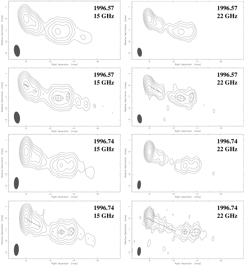
Figure 1: Two epochs of 3C 120 at two frequencies. Images created by cleaning the data (first image of each pair) are directly compared to the images produced by restoring the model-fit components to the transform of the model-fit residuals (second image of each pair). Note the essential similarity of the two sets of images, demonstrating the adequacy of the modeling procedure.

First consider the two components lying in the region between $2$ and $4$ mas from the core, which we have labeled U1A (K1A) and U1B (K1B) in figure 2. They represent easily identifiable discrete structures, and vary smoothly in position, size, flux, and polarization from epoch to epoch, and between our two observing frequencies. Neither is very close to another bright feature. Thus we use these two components to trace motion in the jet of 3C 120.

Next consider the single component that we fit to the region within $2$ mas from the core, which at every epoch is a narrow Gaussian elongated in the direction of the jet. While such a component does represent quite well the flux in this region at each epoch, its parameters are not well determined, and it does not vary smoothly in size, flux, position, or polarization from epoch to epoch, or between frequencies. Therefore we do not attempt to extract any kinematic information from this component.

Finally, there are the several components that we fit beyond $4$ mas from the core. They represent the flux distribution in this part of the jet quite well, but we were unable to extract any kinematic information from them because (i) we cannot reliably identify them between our two frequencies and (ii) there are so many components in one small region that we cannot match them up from epoch to epoch.

Hence there are three types of components that we fit to our sources. The first are well defined, compact, isolated from each other, and clearly identifiable across epoch and frequency. The second are also fit across epochs and frequencies, but do not represent compact structure in the jet. Such components may be marked on our images and discussed in §3, but we do not present formal proper motions for them. The third kind are transitory (present in a few epochs and often at only one frequency), or they are erratic in position, size, flux, and/or polarization (i.e., they “flicker”), or they are simply crowded too close together. While such components surely represent real flux in the jet, we generally do not label them in the images presented in §3, and they are not included in our (very conservative) analysis of jet proper motions.

2.4 Computing Velocities and Accelerations

The proper motions presented in §3 were calculated using the angular component positions in $x$ and $y$ relative to the core component, D. The jets are assumed to be one-sided, and D is taken to be the bright component at the end of the jet. By fitting the motions in $x$ and $y$ independently, we are sensitive to non-radial velocities and accelerations. We use a parameterized model for the motions in ($x$, $y$) that allows us to simultaneously determine three quantities:

• The angular velocity of the component at our middle epoch, $t_{mid}=(t_{min}+t_{max})/2$. This mean velocity should correspond well to the velocity of the component if no acceleration was fit to the data.

• The epoch of origin, $t_{0}$, assuming this mean velocity is constant with no acceleration.

• Any acceleration of the component motion during our observations.

To measure these quantities we developed the following parameterization for motions in ($x$, $y$):

$$x(t)=\mu_{x}(t-t_{x0})+\frac{\dot{\mu}_{x}}{2}(t-t_{mid})^{2}$$ (1)

$$y(t)=\mu_{y}(t-t_{y0})+\frac{\dot{\mu}_{y}}{2}(t-t_{mid})^{2}$$

Thus $\ddot{x}=\dot{\mu}_{x}$ and $\ddot{y}=\dot{\mu}_{y}$ give the angular accelerations. The mean angular velocities, $\dot{x}(t_{mid})=\mu_{x}$ and $\dot{y}(t_{mid})=\mu_{y}$, are given directly, as are the epochs of origin, $t_{x0}=t_{mid}-x(t_{mid})/\dot{x}(t_{mid})$ and $t_{y0}=t_{mid}-y(t_{mid})/\dot{y}(t_{mid})$. These models were fit to our position versus time data using a $\chi^{2}$ minimization routine (Press et al., 1995). In this procedure, the positions measured at the two frequencies were treated independently, giving us $\approx 12$ data points for each component. Our computed proper motions are presented in table 3 as vector proper motions. The reported epochs of origin are an average of $t_{x0}$ and $t_{y0}$ weighted by their uncertainties.

In reporting our measured accelerations in table 3, we resolve the angular accelerations into two components. One component, $\dot{\mu}_{\parallel}$, is along the nominal velocity direction, $\phi$, and represents changes in speed of the component during our observations. The second component, $\dot{\mu}_{\perp}$, is taken along, $\phi+90^{\circ}$, and represents changes in direction of motion during our observations.

The reader will note that the proper motion plots in §3 contain no error bars on the positions of components. We found that no simple rule for estimating positional uncertainties applied well to all components or even to a majority of components. Applying a more detailed procedure, such as manually varying positional parameters for each component while monitoring relative changes in the $\chi^{2}$ statistic, the visual fit with the (u,v)-data, and the flux distribution in the residual image, is a viable solution when a small number of components are involved. However, such a procedure still does not address uncertainties due to fundamental changes in the model (e.g., changes in the number of components fit in a given epoch), possible errors created during the iterative self-calibration and imaging procedure, or jitter in the observed core location. Given these issues and the large number of data points for each component, we decided to use the variance about the best fit to estimate the uncertainties in the fitted parameters. To do this, we initially set the uncertainty for each data point equal to unity. A first pass through fitting our parameterized proper motion model gave a preliminary $\chi^{2}$ value. Taking this preliminary $\chi^{2}$ value, we then uniformly re-scaled the uncertainties on the data points so that $\chi^{2}=N_{points}-N_{parameters}$. A second pass through our fitting procedure then gave us good uncertainty estimates for the velocity, epoch of origin, and acceleration in our models.

As a check on these procedures, we also fit a simpler linear least squares model assuming equally weighted data (no uncertainties on individual points were necessary) and no acceleration. The velocities and epochs of origin (as well their estimated uncertainties) for most components were nearly the same as the values obtained by our more detailed procedure. In a few components, the difference in component velocity and epochs of origin between the two procedures was larger, but was still within the estimated uncertainties.

An interesting statistic is the root mean square variation in position about our fit component trajectories. We computed this statistic with the accelerations set to zero, so the RMS variation is a good upper bound estimate of component position uncertainty and any jitter in the core position (relative to which the component positions are determined). We find the RMS variation in position to be typically $\sim 0.05$ milli-arcseconds with a number of smaller values ($0.02-0.03$ mas) and a few larger values ($0.1-0.2$ mas).

2.5 Conventions and Assumptions

Throughout this paper the structural position angle is denoted by $\theta$, while $\phi$ is the proper motion position angle. Angular separation from the core is denoted by $x$, $y$, and $R=\sqrt{x^{2}+y^{2}}$. Angular proper motion is given by $\mu$ and angular acceleration by $\dot{\mu}$ (for definition of $\dot{\mu}_{\parallel}$ and $\dot{\mu}_{\perp}$ see §2.4). The components are labeled U1 (K1), U2 (K2) $\cdots$ on the 15 GHz (22 GHz) images, in order of emergence, with the earliest labeled U1 (K1). The core is labeled D. Sometimes a component that is picked up beyond U1 (K1) at a later epoch is labeled U0 (K0). In all calculations we assume a Friedman universe with $q_{0}=0.05$ and $H_{0}=100h$ km s^-1 Mpc^-1. Wherever they are discussed in the text, results from the literature have been converted to our choice of cosmology.

Table 3: Proper motion results.

$Object$	$Component$	$N$	$<R>$	$<\theta>$	$\mu$	$\phi$	$\beta_{app}h$	$t_{0}$	$\dot{\mu}_{\parallel}$	$\dot{\mu}_{\perp}$
			(mas)	(deg)	(mas/yr)	(deg)		(years)	(mas/yr/yr)	(mas/yr/yr)
3C 120	K1B/U1B	6	$2.8$	$-112.6\pm 0.3$	$1.62\pm 0.05$	$-102.7\pm 1.5$	$2.5\pm 0.1$	$1994.66\pm 0.10$	$-0.71\pm 0.39$	$0.22\pm 0.32$
	K1A/U1A	6	$3.4$	$-106.8\pm 0.5$	$2.22\pm 0.07$	$-103.7\pm 2.7$	$3.4\pm 0.1$	$1994.90\pm 0.09$	$\underline{-1.37\pm 0.51}$	$-1.10\pm 0.79$
J0530+13	K2/U2	7	$0.2$	$82.7\pm 2.9$	$0.16\pm 0.02$	$43.4\pm 7.3$	$9.7\pm 1.2$	$1995.91\pm 0.21$	$-0.06\pm 0.07$	$0.08\pm 0.07$
J0738+17	K1/U1	6	$0.8$	$79.6\pm 0.7$	$0.14\pm 0.03$	$60.2\pm 10.7$	$2.4\pm 0.4$	$1992.23\pm 1.16$	$-0.39\pm 0.21$	$0.24\pm 0.21$
OJ 287	K3/U3	6	$0.6$	$-94.7\pm 0.6$	$1.01\pm 0.07$	$-90.4\pm 0.9$	$12.8\pm 0.9$	$1995.93\pm 0.10$	$\underline{1.28\pm 0.54}$	$-0.21\pm 0.12$
J1224+21	K3/U3	6	$0.6$	$-13.6\pm 0.5$	$0.65\pm 0.03$	$-9.0\pm 0.8$	$11.2\pm 0.5$	$1995.80\pm 0.07$	$0.18\pm 0.12$	$0.03\pm 0.04$
	K2/U2	6	$1.7$	$-2.5\pm 0.5$	$0.67\pm 0.03$	$-5.3\pm 0.7$	$11.6\pm 0.5$	$1994.53\pm 0.15$	$0.09\pm 0.12$	$0.24\pm 0.03$
	K1/U1	6	$4.7$	$6.3\pm 0.3$	$0.66\pm 0.10$	$-0.6\pm 3.8$	$11.3\pm 1.7$	$1989.78\pm 2.14$	$-0.63\pm 0.40$	$0.15\pm 0.18$
3C 273	K10/U10	5	$0.4$	$-118.1\pm 1.5$	$0.77\pm 0.04$	$-117.4\pm 3.3$	$5.3\pm 0.3$	$1996.12\pm 0.05$	$0.45\pm 0.40$	$-0.05\pm 0.04$
	K9/U9	6	$1.3$	$-121.9\pm 0.7$	$0.94\pm 0.06$	$-120.4\pm 3.2$	$6.5\pm 0.4$	$1995.09\pm 0.13$	$-0.74\pm 0.45$	$0.15\pm 0.39$
	K8/U8	6	$2.0$	$-118.6\pm 0.5$	$1.15\pm 0.05$	$-120.1\pm 2.6$	$8.0\pm 0.3$	$1994.81\pm 0.11$	$-0.07\pm 0.38$	$-0.71\pm 0.40$
	K7/U7	6	$2.7$	$-114.8\pm 0.6$	$1.06\pm 0.08$	$-113.6\pm 4.3$	$7.4\pm 0.6$	$1993.99\pm 0.30$	$\underline{1.30\pm 0.64}$	$-0.60\pm 0.60$
	K4/U4	6	$5.1$	$-111.3\pm 0.2$	$0.99\pm 0.05$	$-120.6\pm 3.2$	$6.9\pm 0.3$	$1991.72\pm 0.34$	$-0.13\pm 0.36$	$-0.54\pm 0.42$
3C 279	K4/U4	5	$0.2$	$-125.1\pm 2.2$	$0.17\pm 0.01$	$-142.4\pm 3.4$	$3.6\pm 0.2$	$1996.09\pm 0.10$	$0.07\pm 0.06$	$0.04\pm 0.05$
	K1/U1	7	$3.1$	$-113.8\pm 0.1$	$0.25\pm 0.01$	$-124.4\pm 1.5$	$5.1\pm 0.1$	$1985.61\pm 0.43$	$-0.06\pm 0.02$	$-0.03\pm 0.02$
J1512$-$09	K2/U2	5	$0.2$	$-32.4\pm 3.0$	$0.19\pm 0.06$	$-24.5\pm 14.6$	$2.8\pm 0.9$	$1995.49\pm 0.52$	$0.36\pm 0.61$	$0.07\pm 0.46$
	K1/U1	6	$1.5$	$-28.6\pm 0.3$	$0.96\pm 0.03$	$-28.2\pm 1.7$	$14.0\pm 0.4$	$1994.93\pm 0.07$	$0.30\pm 0.23$	$0.36\pm 0.22$
J1751+09	K3/U3	6	$0.3$	$31.5\pm 2.3$	$0.45\pm 0.06$	$28.2\pm 5.2$	$5.9\pm 0.8$	$1995.89\pm 0.12$	$-0.26\pm 0.48$	$0.12\pm 0.33$
J1927+73	K3/U3	6	$0.7$	$150.8\pm 0.4$	$0.06\pm 0.02$	$142.8\pm 17.2$	$0.8\pm 0.3$	$1986.37\pm 4.30$	$0.26\pm 0.16$	$0.01\pm 0.14$
	K2/U2	6	$1.8$	$157.3\pm 0.2$	$0.22\pm 0.03$	$164.4\pm 3.1$	$2.8\pm 0.4$	$1987.15\pm 1.36$	$-0.02\pm 0.22$	$0.30\pm 0.09$
	K1/U1	6	$2.1$	$172.9\pm 0.1$	$0.25\pm 0.02$	$168.9\pm 3.8$	$3.1\pm 0.3$	$1989.06\pm 1.12$	$\underline{0.40\pm 0.18}$	$-0.10\pm 0.13$
J2005+77	U3	6	$0.2$	$-84.3\pm 4.3$	$0.04\pm 0.03$	$-58.9\pm 33.0$	$0.5\pm 0.4$	$\cdots$	$\cdots$	$\cdots$
	U2	6	$0.5$	$-93.4\pm 0.7$	$0.02\pm 0.02$	$137.5\pm 62.0$	$0.2\pm 0.2$	$\cdots$	$\cdots$	$\cdots$
	U1	6	$1.7$	$-93.3\pm 0.5$	$0.20\pm 0.04$	$172.2\pm 13.9$	$2.8\pm 0.6$	$\cdots$	$\cdots$	$\cdots$

Note. — The number of epochs are given by $N$. Mean-epoch values for angular radius, $<R>$, and structural position angle, $<\theta>$, are provided for comparison. Proper motion and structural position angles are measured to be positive, counter-clockwise from north. See §2.5 for a general discussion of our conventions and §2.4 for a detailed discussion of our proper motion fitting procedure.

3 Results

In this section we present our observed proper motions for the well-defined components in each source. Complete model fitting results as well as images of all sources at both frequencies and all epochs will be presented in Ojha et al. (in prep). Here we present a single total intensity image for each source, labeling the components that are discussed in the text. We also show a plot of angular radial distance, $R$, versus time for all components for which we present proper motions. When appropriate to understanding a particular component’s motion, we also present plots of the angular position ($x$, $y$) over time. Table 3 contains a summary of the computed proper motions for each source in our sample (see §2.4). On all of our plots (($R$, $t$) and ($x$, $y$)) we overlay a projection of these fitted proper motions. The trajectories may be non-radial and include accelerations; therefore, the projections of these motions will not, in general, be straight lines.

3.1 3C 120 (J0433$+$05)

3C 120 is a nearby example of extra-galactic superluminal motion (Seielstad et al., 1979). At a redshift of just $0.033$, an observed proper motion of $1$ mas/yr corresponds to a speed of $1.5h^{-1}$c. Recent results from Gomez et al. (1998) at 22 and 43 GHz show up to 10 superluminal components with angular velocities between $1.5$ mas/yr ($2.3h^{-1}$c) and $3.6$ mas/yr ($5.5h^{-1}$c).

While, in any given epoch, we observe a large number of components (regions of enhanced brightness) in the jet, we found it very difficult to identify many of these components across epochs and (to a lesser extent) across frequency (see §2.3). The components U1A (K1A) and U1B (K1B) (see figure 2), however, are unambiguously identified in all epochs and at both frequencies. Our computed proper motions for U1A (K1A) and U1B (K1B) appear in table 3. Figure 3 shows the radial position of these components versus time with the fitted proper motions superimposed.

Figure 2: Total intensity image of 3C 120 at 15 GHz, epoch 1996.57. Components discussed in the text are marked on the image. Contours begin at 2 mJy/beam and increase in $\sqrt{2}$ steps.

Figure 3: Radial position of model components versus time for 3C 120. Components U1A (K1A) and U1B (K1B) are plotted with their fitted motion lines. Components are marked with a “$\blacklozenge$” at $15$ GHz and a “$\bigcirc$” at $22$ GHz. Components that we do not follow well enough to present proper motions for are included on the plots marked with a “$\times$” at $15$ GHz and a “$+$” at $22$ GHz.

At $2.22\pm 0.07$ and $1.62\pm 0.05$ mas/yr for U1A (K1A) and U1B (K1B) respectively, the proper motions of these components are distinctly different; however, their epochs of origin are nearly the same, straddling $1994.8$. Figures 4 and 5 show the detailed ($x$, $y$) motion of these components over time. The proper motion position angles of both components ($\phi\simeq-103^{\circ}$) are nearly along the local jet direction; however, for component U1B (K1B) this proper motion position angle is $10^{\circ}$ from its structural position angle relative to the core ($-113^{\circ}$) and is distinctly non-radial. An interesting aspect of the motion of U1A (K1A) is that it appears to slow down over time (see figure 4); we measure this deceleration to be $-1.37\pm 0.51$ mas/yr/yr, a $2.6\sigma$ result.

Figure 4: Plot showing the $x$ and $y$ position from the core of component U1A (K1A) in 3C 120. The six epochs are labeled A through F with the capitals referring to the higher frequency. The solid line is the projection of the derived motion of U1A (K1A). The dotted line is line for pure radial motion. The derived motion is not significantly non-radial. Note the apparent deceleration in the motion of U1A (K1A).

Figure 5: Plot showing the $x$ and $y$ position from the core of component U1B (K1B) in 3C 120. The six epochs are labeled A through F with the capitals referring to the higher frequency. The solid line is the projection of the derived motion of U1A (K1A). The dotted line is line for pure radial motion. The derived motion is significantly non-radial.

3.2 J0530+135 (B0528+134)

This EGRET-detected quasar varies with extreme rapidity at high energies (Mukherjee et al., 1996). It is also well known as a strong, flat spectrum radio source (Aller et al., 1985). At a redshift of 2.060, proper motion of $1$ mas/yr corresponds to a velocity $60.3h^{-1}$ times the speed of light. Global VLBI observations at 8 and 22 GHz (Pohl et al., 1996, 1995) found one component moving at a superluminal speed of $\beta_{app}h=6.6\pm 2.6$ ($\mu=0.11\pm 0.043$ mas/yr). Britzen et al. (1999), observing at 8 GHz, model up to seven jet features, finding superluminal motion of about $7-9h^{-1}$c ($\mu=0.12-0.15$ mas/yr) for five of them. They report that the two outermost components show higher speeds than do the inner five. Further, they find that some of their components move along curved trajectories that differ from component to component. The ejection position angles of two pairs of components are displaced by about $100^{\circ}$. They find that the times of ejection coincide with the beginning of “phases of enhanced flux-density activity” for four components.

Our images are the first VLBP (Very Long Baseline Polarization) images of this source. The total intensity structure is in agreement with earlier VLBI images. We see a faint jet extending up to 3 mas from the core. To our data we fit a core and two jet components within the first milliarcsecond of the jet. Almost all the flux is contained in the core and innermost component (see figure 6). While this is the simplest model that adequately fits the total intensity observations, it is almost certainly not a complete description of the source whose complexity is more apparent in our polarized images (Ojha et al., in prep.).

Figure 6: Total intensity image of J0530+13 at 22 GHz, epoch 1996.57. Components discussed in the text are marked in the image. The contours begin at 15 mJy/beam and increase in $\sqrt{2}$ steps.

Figure 7: Radial position of model components versus time for J0530+13. Component K2 (U2) is plotted with its fitted motion line. Components are marked with a “$\blacklozenge$” at $15$ GHz and a “$\bigcirc$” at $22$ GHz. Components that we do not follow well enough to present proper motions for are included on the plots marked with a “$\times$” at $15$ GHz and a “$+$” at $22$ GHz.

The outer-most component K1 (U1) has no clear proper motion (see figures 7 and 8) and is fit closer to the core at the higher frequency at every epoch, suggesting a strong spectral index gradient. This feature is large (about 0.5 mas in size) and the differences in position at the different frequencies are smaller than its size. Thus it could be a single component with a large gradient in spectral index; however, its shape and orientation vary enough that it cannot be considered a well defined component, and we do not use it in our kinematic analysis.

The behavior of the inner component K2 (U2) lends itself to two different interpretations. If we interpret all 7 epochs (times 2 frequencies) as the motion of a single component, we obtain a proper motion of $0.16\pm 0.02$ mas/yr, corresponding to $\beta_{app}h=9.7\pm 1.2$ (figure 7). The derived motion is clearly non-radial (figure 8) at a proper motion position angle that differs from its mean structural position angle by at least $30^{\circ}$. The proper motion position angle is approximately along a line from K2 (U2) toward K1 (U1).

Figure 8: Plot showing the $x$ and $y$ position from the core of components K1 and K2 in J0530+13. The seven epochs are labeled A through G with the capitals referring to the higher frequency. Note that the position of K1 (upper left) varies erratically with epoch and frequency supporting the interpretation that it is not a discrete component. In contrast, the position of the well-defined component K2 (close to origin) hangs together well. The non-radial nature of K2’s motion stands out in this plot.

Examining our data, however, it is clear that our independent fits for K2 (U2) at 15 and 22 GHz agree very closely at every epoch from 1996.22 onward, and it seems unlikely that modeling error will cause the “jittery” variation in position that we see in figure 7. In addition to the positional variation, we see accompanying changes in the flux of K2 (U2) between epochs 1996.22 and 1996.41 that suggest we may not be looking at the same component at the two epochs (Ojha et al., in prep.). Its flux rises sharply from $\sim$$1.5$ to $\sim$$4.0$ Jy at both frequencies, while that of the core drops from $\sim$$7.8$ to $\sim$$3.9$ Jy. This change in flux is not an artifact of our model fitting and is confirmed by changes in our polarization images. Taking just the epochs 1996.41 through 1996.74, we would fit a component moving on a well-defined trajectory with a proper motion of more than $20h^{-1}$c! However, at the next epoch, 1996.93, we observe K2 (U2) falling short of the predicted position for such a fast motion. We may be seeing the effects of a curving jet trajectory, multiple component ejection and the limits of our spatial and temporal resolution. We consider the simple interpretation of a single component trajectory to be the minimum motion exhibited by the feature(s) we call K2 (U2), and this is the motion we report in table 3.

3.3 J0738+177 (B0735+178)

This highly optically variable BL Lac object has one of the most bent jets on milliarcsecond scales (Gabuzda et al., 1994). With an absorption line redshift of $0.424$, proper motion of 1 mas/yr corresponds to a velocity of at least $16.9h^{-1}$c. Bååth & Zhang (1991) reported superluminal motion in a component of $\sim 7.9h^{-1}$c ($\sim 0.47$ mas/yr). Gabuzda et al. (1994) confirmed the motion of this component at a velocity $8.1h^{-1}$c ($0.48\pm 0.02$ mas/yr), reported speeds of $5.6h^{-1}$c ($0.33\pm 0.02$ mas/yr) and $4.7h^{-1}$c ($0.28\pm 0.03$ mas/yr) for two other components, and found evidence for a stationary component with $\mu=0.03\pm 0.04$ mas/yr.

We see most of the flux in an East-West core-jet, plus a faint parallel “bar” of emission, about 1.5 mas north of the main structure. This unusual morphology is also seen by Kellermann et al. (1998) and Gomez et al. (1999). Our fitting process yields one reliable jet component, U1 (K1), at $R\simeq 0.8$ mas and $\theta\simeq$ 80^∘ (see figure 9), that is consistently fit over all epochs at 15 GHz but only at the first two epochs at 22 GHz, probably due to the lack of sensitivity at the higher frequency. Gomez et al. (1999) propose that this component marks a bend in the jet. However, we find no evidence of anything other than the unaccelerated, essentially radial motion reported in table 3 and figure 10 of $\beta_{app}h=2.4\pm 0.4$ ($\mu=0.14\pm 0.03$ mas/yr).

Figure 9: Total intensity image of J0738+17 at 15 GHz, epoch 1996.05. Components discussed in the text are marked on the image. Contours begin at 3 mJy/beam and increase in $\sqrt{2}$ steps.

Figure 10: Radial position of model components versus time for J0738+17. Component U2 (K2) is plotted with its fitted motion line. Components are marked with a “$\blacklozenge$” at $15$ GHz and a “$\bigcirc$” at $22$ GHz. Components that we do not follow well enough to present proper motions for are included on the plots marked with a “$\times$” at $15$ GHz and a “$+$” at $22$ GHz.

We also find a second component, U2 (K2), close to the core. This component seems to change its size, shape, flux, and position in unpredictable ways from epoch to epoch. Its angular size was often much larger than its separation from the core and oriented along its structural position angle. For these reasons we do not present a proper motion for it. The only thing consistent about U2 (K2) is its structural position angle of $50-55^{\circ}$ which is distinctly different from that of U1 (K1).

We were unable to fit any reproducible components to the bar of emission to the north, and cannot address proper motions in this region of the jet.

3.4 OJ 287 (J0854+201, B0851+202)

OJ 287 is a BL Lac object at a redshift of 0.306, where $1$ mas/yr corresponds to an apparent speed of $12.7h^{-1}c$. Its VLBI structure has been studied at centimeter wavelengths by the Brandeis Radio Astronomy Group for about 17 years (Roberts, Gabuzda & Wardle, 1987; Gabuzda, Wardle, & Roberts, 1989; Gabuzda & Cawthorne, 1996). They report a proper motion of $\sim 0.25$ mas/yr for two components. Vicente, Charlot, & Sol (1996) report a proper motion as high as $0.4$ mas/yr for their component K3. Tateyama et al. (1999) report an average speed of about $0.5$ mas/yr for six components that they follow.

Our analysis of OJ 287 provides an excellent example of the need for frequent (no less often than bi-monthly) monitoring of such sources, as well as of the importance of polarization images in deciphering the kinematics of blazars. In any given epoch OJ 287 exhibits a simple total intensity structure, with a strong core and a short parsec scale jet extending almost due west (figure 11). The structure and polarization of our images are consistent with the near-simultaneous 43 GHz image of Lister, Marscher, & Gear (1998). The jet is well fit by two or three components at every epoch. However, our closely-separated epochs reveal complex kinematics that would have been missed by less well sampled observations, and without the polarization images of the components, we could not have understood the situation with confidence.

Figure 11: Total intensity image of OJ 287 at 22 GHz, epoch 1996.57. Components discussed in the text are marked on the image. Contours begin at 2 mJy/beam and increase in $\sqrt{2}$ steps.

Figure 12: Radial position of model components versus time for OJ 287. Component K3 (U3) is plotted with its fitted motion line (solid line). Components are marked with a “$\blacklozenge$” at $15$ GHz and a “$\bigcirc$” at $22$ GHz. Components that we do not follow well enough to present proper motions for are included on the plots marked with a “$\times$” at $15$ GHz and a “$+$” at $22$ GHz. The motion of K3 (U3) is clearly affected by its proximity to (the as yet unresolved) component K4 in the first three epochs resulting in the apparent “jump” in its position between the third and fourth epochs.

Of the three components that make up the jet, K2 (U2) and K4 (U4) show no significant outward motion, while K3 (U3) moves radially outward with an apparent speed of $1.01\pm 0.07$ mas/yr ($\beta_{app}h=12.8\pm 0.9$) and emergence date $1995.93\pm 0.10$ (figure 12). The difficulty in discovering this behavior arises from the fact that K3 (U3) passes successively through K4 (U4) and K2 (U2) in its outward motion. For the first two epochs we do not fit K4 (U4), and for the last two epochs we do not fit K2 (U2), as during these epochs K3 (U3) is effectively merged with K4 (U4) or K2 (U2) respectively. This merging may bias slightly the position of K3 (U3) at these times, and leads to the borderline significant acceleration fit to K3 (U3). The key to identifying this picture is that K3 (U3) has distinctive polarization properties, particularly its polarization position angle, that it maintains over all the epochs (see figure 13). The polarization position angle of K3 (U3) is aligned neither parallel nor perpendicular to the jet axis, but at an oblique angle to both its structural position angle and the direction of its proper motion. The component fits agree closely between our two frequencies, both in the position and polarization of K3 (U3). By epoch 1997.94, K3 (U3), along with its peculiar mis-aligned polarization, has disappeared, which we would expect given that its speed would place it beyond the point in the jet of OJ 287 where the brightness sharply falls off at 15 and 22 GHz ($\sim 2$ mas).

Figure 13: Total intensity (panel a) and polarization (panel b, tick marks indicate electric vector direction) images of OJ 287 at 15 GHz. The approximate locations of the core and component U3 (K3) are marked on the images. As detailed in the text, the persistent polarization properties of U3 (K3) were the important clues that allowed us to confidently identify it across epoch.

To illustrate the complex problem of discovering the motion of K3 (U3), we show in figure 13a the 15 GHz total intensity images of OJ 287 during 1996. On each panel we have marked the approximate positions fit to the total intensity distributions of the core and component U3. We have marked these same positions in figure 13b, which shows the polarization images for each epoch. It is clear that component U3 (K3) maintains the same polarization structure throughout our observations. While it is true that the location of the polarization peaks do not precisely match those of the total intensity component, they are well within a beam width of one another. In the early epochs, this displacement is clearly due to “beating” with the polarization of the core component. Our component model-fits, which require the polarization to be fit at the location of the total intensity components and are less subject to “beating” effects, show this polarization structure to be always part of component U3 (K3).

3.5 J1224+212 (B1222+216, 4C 21.35)

J1224+212 is one of the most distorted of the WAT (wide-angle-tailed) quasars (Hintzen, 1984; Saikia, Wiita & Muxlow, 1993). At a redshift of 0.435, an observed proper motion of $1$ mas/yr corresponds to an apparent speed of $17.3h^{-1}$ times the speed of light. Hooimeyer et al. (1992), report a tentative detection of superluminal proper motion of $\beta_{app}h=1.6\pm 0.6$ ($0.09\pm 0.04$ mas/yr) for a component located $\sim$$3$ mas from the core.

Figure 14: Total intensity image of J1224+21 at 22 GHz, epoch 1996.57. Components discussed in the text are marked on the image. Contours begin at 3 mJy/beam and increase in $\sqrt{2}$ steps.

Our images show a dominant core and a north-south jet (figure 14), in general agreement with Hooimeyer et al. (1992). Using our two frequencies we are able to follow confidently the motion of three jet components. The proper motions of K1 (U1), K2 (U2) and K3 (U3) are highly superluminal with $\beta_{app}h=$ $11.3\pm 1.7$, $11.6\pm 0.5$ and $11.2\pm 0.5$ respectively (figure 15). These components are located at differing structural position angles increase from $-14^{\circ}$ to $+6^{\circ}$ with increasing radius. The proper motion position angles of these components also increase from $\phi\simeq-9^{\circ}$ to $\phi\simeq-1^{\circ}$ with radius. Interestingly, component K2 (U2) shows a significant perpendicular acceleration $\dot{\mu}_{\perp}=0.24\pm 0.03$ (see figure 16) which is consistent with this change in position angle with radius. Both K3 (U3) and K2 (U2) show slight, but significant, non-radial motions; however, the apparent position of K3 (U3) may be biased (particularly at U-band where U4 is not fit until 1997.94) by its close proximity to the core, combined with the emergence of component K4 (U4). Component K4 is fit close to the core and is $\lesssim 15$% of the core flux; combined with its large size ($\sim 0.5$ mas) relative to its core separation ($\sim 0.1$ mas), we did not feel that the motion of K4 could be followed robustly during 1996. Only in 1997.94, is K4 (U4) clearly separated from the core. A naive fit, including the 1996 points, is included in figure 15 as a dotted line and suggests strong acceleration with $\mu=0.35\pm 0.01$ mas/yr and $\dot{\mu}_{\parallel}=0.66\pm 0.09$ mas/yr/yr.

Figure 15: Radial position of model components versus time for J1224+21. Components K4 (U4), K3 (U3), K2 (U2), and K1 (U1) are plotted with their fitted motion lines. Components are marked with a “$\blacklozenge$” at $15$ GHz and a “$\bigcirc$” at $22$ GHz. Components that we do not follow well enough to present proper motions for are included on the plots marked with a “$\times$” at $15$ GHz and a “$+$” at $22$ GHz.

Figure 16: Plot showing the $x$ and $y$ position from the core of component K2 (U2) in J1224+21. The six epochs are labeled B through G with the capitals referring to the higher frequency. The line of best fit indicates a significant perpendicular acceleration in the component motion.

3.6 3C 273 (J1229+02)

The famous quasar 3C 273 is one of the best studied AGN in all wavebands. The source has been observed with VLBI techniques for over 30 years. At a redshift of 0.158, a proper motion of $1.0$ mas/yr corresponds to an apparent proper motion of $7.0h^{-1}$ c. Abraham et al. (1996) examine all the available data in the literature including their own observations up to early 1991. They find that the velocities of individual components do not change with time; however, the proper motions can be distinctly different from component to component with a range of $0.7$ to $1.2$ mas/yr.

We follow five components in the first 6 mas of the jet with sufficient confidence to compute their proper motions. We have labeled these components K4, K7, K8, K9, and K10 in figure 17, and their proper motions are listed in table 3. Figure 18 shows the radial position versus epoch for each of these components. The oldest of these components, K4 (U4), has an epoch of emergence that is later than any of the observations summarized and reported by Abraham et al. (1996), so no identification with the components they track is possible.

Figure 17: Total intensity image of 3C 273 at 22 GHz, epoch 1996.93. Components discussed in the text are marked on the image. Contours begin at 20 mJy/beam and increase in $\sqrt{2}$ steps.

Figure 18: Radial position of model components versus time for 3C 273. Components K10 (U10), K9 (U9), K8 (U8), K7 (U7), and K4 (K4) are plotted with the projections of their computed motions. Components are marked with a “$\blacklozenge$” at $15$ GHz and a “$\bigcirc$” at $22$ GHz. Components that we do not follow well enough to present proper motions for are included on the plots marked with a “$\times$” at $15$ GHz and a “$+$” at $22$ GHz.

As reported in table 3, the proper motions of the components we follow range from $0.77$ to $1.15$ mas/yr ($\beta_{app}h=5.3$ to $6.9$), and their structural position angles range from $-111^{\circ}$ to $-122^{\circ}$. A number of authors have noted a “wiggling” in the ridge line of the milli-arcsecond jet of 3C 273 (Zensus et al., 1990; Krichbaum et al., 1990; Bååth et al., 1991; Leppännen, Zensus & Diamond, 1995; Mantovani et al., 1999). While we do fit differing structural position angles for our components, it is interesting that the component motions do not appear to follow this “wiggle”. We find that the proper motions for all components, with the exception of K4 (U4), are consistent with radial motion along their structural position angles. Component K4 (U4) has a fitted proper motion position angle of $-120.6^{\circ}\pm 3.2^{\circ}$ as compared to its mean structural position angle of $-111.3^{\circ}\pm 0.2^{\circ}$ (see figure 19); these values differ at nearly the three sigma level, suggesting non-radial motion.

Figure 19: Plot showing the $x$ and $y$ position from the core of component K4 (U4) in 3C 273. The six epochs are labeled A through F with the capitals referring to the higher frequency. The line of best fit indicates borderline significant non-radial motion.

3.7 3C 279 (J1256$-$05)

Another famous quasar, 3C 279, has also been studied for $\sim$30 years with VLBI techniques. At a redshift of $0.536$, $1$ mas/yr corresponds to an observed proper motion of $20.6h^{-1}$ times the speed of light. Cotton et al. (1979) measured an expansion speed of $0.5$ mas/yr along a position angle of $-140^{\circ}$. Unwin et al. (1989) follow a component they call “C3” with a proper motion of $0.12\pm 0.02$ mas/yr along a position angle of $-134^{\circ}$. Carrara et al. (1993) have additional observations of “C3,” and revise this proper motion to $0.16\pm 0.01$ mas/yr; they also observe a proper motion for a component denoted “C4” of $0.15\pm 0.01$ mas/yr along a position angle of about $\sim-114^{\circ}$. The same “C4” is apparently followed by Unwin et al. (1998) over a much longer period of time with a proper motion of $\simeq 0.24$ mas/yr.

We observe only the inner $3$ mas of the jet in 3C 279, and identify four components (labeled U1-U4 in figure 20) in each of our epochs. Of these components, only U1 (K1) and U4 (K4) have well defined proper motions at both frequencies. U1 (K1) is the same component “C4” followed by Unwin et al. (1998). Component U2 (K2) appears to be a strong but poorly defined “tail” to U1 (K1) (see figure 22). Component U3 (K3) is not a well defined component and may represent some underlying jet emission.

Figure 20: Total intensity image of 3C 279 at 15 GHz, epoch 1996.74. Components discussed in the text are marked on the image. Contours begin at 30 mJy/beam and increase in $\sqrt{2}$ steps.

Figure 21: Radial position of model components versus time for 3C 279. Components U4 (K4) and U1 (K1) are plotted with their fitted motion lines. Components are marked with a “$\blacklozenge$” at $15$ GHz and a “$\bigcirc$” at $22$ GHz. Components that we do not follow well enough to present proper motions for are included on the plots marked with a “$\times$” at $15$ GHz and a “$+$” at $22$ GHz.

Our fit to the proper motion of U1 (K1) is reported in table 3 and plotted in figure 21. We find a proper motion of $0.25\pm 0.01$ mas/yr, in agreement with Unwin et al. (1998). The proper motion of U1 (K1) is distinctly non-radial (see figure 22) with a proper motion position angle of $-124^{\circ}\pm 2^{\circ}$ as compared to its mean structural position angle of $-114^{\circ}$. This non-radial motion is paired with a slight (but significant) deceleration of the component of $-0.06\pm 0.02$ mas/yr/yr. Both the non-radial motion and deceleration may result from either an interaction of U1 (K1) with the external medium or the “tail” component U2 (K2) catching up with U1 (K1). This scenario is suggested by the observation that the flux of U1 (K1) rose by nearly $50\%$ from epoch 1996.93 to epoch 1997.94 while the flux of U2 (K2) fell off significantly (Ojha et al., in prep.).

Figure 22: Plot showing the $x$ and $y$ position from the core of components U1 (K1) and U2 (K2) in 3C 279. The seven epochs are labeled A through G, with the capitals referring to the higher frequency. The positions of the well-defined component U1 (K1) (upper right) are plotted against its projected motion which is clearly non-radial. The positions of U2 (K2) are scattered showing how poorly this “tail” component is followed.

Component U4 (K4) is a developing component very near the core of the jet that rises sharply in flux during our observations and has polarization properties distinct from those of the core (Ojha et al., in prep.). We fit what appears to be a strongly accelerated motion for U4 (K4), with $\dot{\mu}_{\parallel}=0.24\pm 0.04$ mas/yr/yr along the component motion, so that over the two year span of our observations, its speed changes by more than twice the average velocity of $0.11\pm 0.01$ mas/yr. This component is also moving non-radially along a position angle of $-148.2^{\circ}\pm 5.3^{\circ}$ which differs from its structural position angle by more than $20^{\circ}$. There is a slight, bending acceleration to the component motion of $\dot{\mu}_{\perp}=0.08\pm 0.03$ mas/yr/yr which may be related to this non-radial motion. Figure 23a displays this fitted motion on the ($x$, $y$) position plot of U4 (K4) over time. This plot immediately raises some issues for our fitted motion. It appears as though the position of the component during the first two epochs (A and B) is inconsistent with the motion suggested by the remaining epochs. As stated above, component U4 (K4) rises sharply in flux during our observations, and has its lowest flux states during the first two epochs. At 22 GHz, K4 is only $13$% of the core flux in epoch A and is only $25$% of the core flux in epoch B. This component is large enough in size ($0.3-0.4$ mas FWHM) that biasing due to the proximity and strong relative flux of the core in these epochs is a concern. By the later epochs, U4 (K4), is comparable in strength to the core, and its position is less likely to be seriously biased by the presence of the strong core.

Figure 23: Plots showing the $x$ and $y$ position from the core of component U4 (K4) in 3C 279. The seven epochs are labeled A through G, with the capitals referring to the higher frequency. Panel (a) displays the best fit to all seven epochs while panel (b) excludes the first two epochs.

In figure 23b, we show the component motion without the first two epochs contributing to the fit. Here we find a motion $\mu=0.17\pm 0.01$ mas/yr along a position angle of $-142.4^{\circ}\pm 3.4^{\circ}$. This motion is still significantly non-radial by $\approx 17^{\circ}$ but has no significant acceleration, $\dot{\mu}_{\parallel}=0.07\pm 0.06$ mas/yr/yr. This result is more conservative and we report it in table 3 and plot it in figure 21; however, it is possible that figure 23a represents the correct motion for component U4 (K4), with the component maintaining a distance of $0.1\pm 0.05$ mas from the core during 1996 and accelerating to $0.3$ mas by the end of 1997.

3.8 J1310+323 (B1308+326, OP 313)

This source is a resolved blob in our VLBI images, and although we have been able to model this source with multiple components, we cannot identify components over epochs or between frequencies. Hence no information about its proper motion is presented.

3.9 J1512$-$090 (B1510$-$089, OR $-$017)

This fascinating source is discussed in detail in Wardle et al. (in preparation). It is one of the most violently variable examples of an OVV blazar (Moore & Stockman, 1984). It is also classified as a radio selected quasar by Hewitt & Burbidge (1993). At a redshift of $0.360$, $1$ mas/yr corresponds to an observed proper motion of $14.6h^{-1}$ times the speed of light. Fey & Charlot (1997) have VLBI images at three frequencies that show a strong core containing most of the flux and a jet extending northwest. Bondi et al. (1996) have images at three epochs with a jet extending to the south! There is, however, an extension to the north corresponding to the Fey & Charlot (1997) jet.

The total intensity structure we observe (see figure 24) is similar to the Fey & Charlot (1997) 15 GHz image, with a strong core and a jet along $\theta\approx-30$ degrees. We fit the source with a core and two jet components.

Figure 24: Total intensity image of J1512$-$09 at 15 GHz, 1996.41. Components discussed in the text are marked on the image. Contours begin at 3 mJy/beam and increase in $\sqrt{2}$ steps.

The proper motions for the two jet components are reported in table 3 and displayed in figure 25. The outer jet component K1 (U1) is moving radially at an astonishing $\beta_{app}h=14.0\pm 0.4$ ($0.96\pm 0.03$ mas/yr) making it the fastest superluminal component in our sample. This component also appears to be expanding in angular size at superluminal speed (Wardle et al., in preparation). Much closer to the core, component K2 (U2) is also moving radially at the considerably slower speed of $\beta_{app}h=2.8\pm 0.9$ ($0.19\pm 0.06$ mas/yr). We detect no non-radial motions or accelerations in the individual motions of these components.

Figure 25: Radial position of model components versus time for J1512$-$09. Components U2 (K2) and U1 (K1) are plotted with their fitted motion lines. Components are marked with a “$\blacklozenge$” at $15$ GHz and a “$\bigcirc$” at $22$ GHz. At $\beta_{app}h=14.0\pm 0.4$, U1 (K1) is the fastest superluminal component in our sample.

3.10 J1751+09 (B1749+096, OT 081, 4C 09.56)

This compact BL Lacertae object has a redshift of $0.322$, so an observed proper motion of 1 mas/yr corresponds to an apparent speed of $13.2h^{-1}$ times the speed of light. At milliarcsecond scales over $90$% of its flux is contained within a compact component $\sim 0.2$ mas in size (Weiler & Johnston, 1980). Wehrle et al. (1992) report a strong compact source with an emission to the north. Fey, Clegg & Fomalont (1996) have VLBI images at four frequencies also showing this northward extension, with over 90 percent of the flux in the compact core. Gabuzda & Cawthorne (1996) and Gabuzda, Pushkarev & Cawthorne (1999) see a compact jet initially at $\theta=25^{\circ}$ that curves to the south.

Our image (figure 26) shows a very compact core containing over 95% of the flux and an extension at $\theta\simeq 30^{\circ}$. At 22 GHz we fit only a single Gaussian component at the core. At 15 GHz, however, we fit a component close to the core, labeled U3 in figure 26, that has a proper motion of $0.45\pm 0.06$ mas/yr (figure 27). The flux of this component falls off very rapidly as it moves away from the core (Ojha et al., in prep.). Because of its close proximity to the core and rapid fall-off in flux, the proper motion of U3 may be confused by the presence of the variable core. We detect no non-radial motion or acceleration here.

Figure 26: Total intensity image of J1751+09 at 15 GHz, epoch 1996.57. Components discussed in the text are marked on the image. Contours begin at 2 mJy/beam and increase in $\sqrt{2}$ steps.

Figure 27: Radial position of model components versus time for J1751+09. Component U3 is plotted with its fitted motion line. Components are marked with a “$\blacklozenge$” at $15$ GHz. Note the large change in position between epochs 1996.41 and 1996.57 as U3 moves away from the influence of the strong core.

3.11 J1927+739 (B1928+738, 4C 73.18)

This OVV quasar is at a redshift of $0.302$ where a proper motion of 1 mas/yr corresponds to an apparent speed of $12.4h^{-1}$c. Eckart et al. (1985, 1987) and Witzel et al. (1988), observing at 5 GHz, find a complex jet extending $\sim 20$ mas to which they fit nine components of which at least five are superluminal, with $\beta_{app}h$ ranging from $4$ to $8$ ($0.3-0.6$ mas/yr). Eckart et al. (1985) draw attention to the fact that the jet is not straight and the structural position angles of the components vary from $151^{\circ}$ to $175^{\circ}$ as seen from the core. Six epochs of $22$ GHz images made by Hummel et al. (1992) show three superluminal components, one of which may be exhibiting acceleration between epochs, with a velocity of about $4h^{-1}$c ($0.34$ mas/yr). They refer to work by Schalinski (at 5 GHz) showing an average superluminal velocity of $\sim 7h^{-1}$c and point out that taken in conjunction with their results, this indicates acceleration between the $\sim 2$ mas and the $6-15$ mas scales.

We fit this source with a core and three well defined jet components (figure 28), for which proper motions are displayed in figure 29 and reported in table 3. Components K2 (U2) and K1 (U1) are located at what might be visually interpreted as two sharp bends in the jet; however, they are both moving predominantly radially (the motion of K2 (U2) has a small non-radial component which is significant at the $2\sigma$ level) away from the core at $\beta_{app}h=2.8\pm 0.4$ and $3.1\pm 0.3$, respectively (figure 30). About $0.7$ mas from the core, we fit a third component, K3 (U3), that has a distinctly slower radial motion of $\beta_{app}h=0.8\pm 0.3$.

Figure 28: Total intensity image of J1927+73 at 22 GHz, epoch 1996.23. Components discussed in the text are marked on the image. Contours begin at 5 mJy/beam and increase in $\sqrt{2}$ steps.

Figure 29: Radial position of model components versus time for J1927+73. Components K3 (U3), K2 (U2), and K1 (U1) are plotted with their fitted motion lines. Components are marked with a “$\blacklozenge$” at $15$ GHz and a “$\bigcirc$” at $22$ GHz.

Figure 30: Plot showing the $x$ and $y$ position from the core of components K2 (U2) and K1 (U1) in J1927+73. The six epochs are labeled A through F, with the capitals referring to the higher frequency.

The differing structural position angles of all three components, coupled with their predominantly radial motions, suggests that there may be different angles of ejection for different components in this jet. An interesting fact is that K2 (U2), in addition to having a slightly significant non-radial motion, has a significant bending acceleration of $0.30\pm 0.09$ mas/yr/yr, in the right direction to bring the trajectory of K2 (U2) parallel to that of K1 (U1). Thus it is possible that we are seeing the effects of collimation here.

In figure 30, it is interesting to note the location of the components in epoch “C” (1996.41). Relative to the motion suggested by the other epochs, the ($x$, $y$) positions of both K1 (U1) and K2 (U2) in epoch “C” are clearly displaced toward the core by the same amount. This could well be due to variation in the observed core position, against which all the component positions are determined. Also note that the higher frequency is systematically fit at a larger radii for both components at most epochs. This systematic position shift is also apparent in figure 29 for component K3 (U3). Both pieces of evidence suggests a core shift between $15$ and $22$ GHz of $\sim 0.04$ mas.

3.12 J2005+778 (B2007+777)

This source is unique as the only source in our sample whose components show no discernible proper motions. The process of modeling and understanding this source was also a reminder of the pitfalls of modeling single frequency observations – our 22 GHz modeling by itself leads to an interpretation that is plausible but probably incorrect.

J2005+778 is a BL Lacertae object at a redshift of 0.342 where a proper motion of 1 mas/yr corresponds to an apparent speed of $14h^{-1}$c. VLBI images by Eckart et al. (1987) and Witzel et al. (1988) show a jet at $\theta\simeq-95^{\circ}$. They identify a component that has a proper motion of $0.18$ mas/yr, corresponding to $\beta_{app}h=2.5$. Gabuzda et al. (1994) see a similar structure and fit their image with six components. By identifying one of their components with that of Eckart et al. (1987) and Witzel et al. (1988), they calculate a proper motion of $0.22\pm 0.02$ mas/yr, corresponding to $\beta_{app}h=3.1\pm 0.8$ over $\sim 9$ years.

Our images (see figure 31) show a jet extending $\sim 2.5$ mas at $\theta\simeq-95^{\circ}$. At 22 GHz the data appear to be well fit with three components, the core, K1, and K2. If we confine our analysis to 22 GHz, we find that K1 and K2 are moving with jerky but distinctly superluminal apparent speeds comparable to those found by Gabuzda et al. (1994) (see figure 32).

Figure 31: Total intensity image of J2005+77 at 15 GHz, epoch 1996.23. Components discussed in the text are marked on the image. Contours begin at 2 mJy/beam and increase in $\sqrt{2}$ steps.

Figure 32: Radial position of model components versus time for J2005+77. Components U3, U2, and U1 are plotted with their fitted motion lines. Within our uncertainties, these components do not propagate down the jet. Components are marked with a “$\blacklozenge$” at $15$ GHz. Components that we do not follow well enough to present proper motions for are included on the plots marked with a “$+$” at $22$ GHz.

At 15 GHz, the core region is fit with two components, D and U3. All the jet components, U1, U2, and U3 are stationary in the radial direction (motions are listed in table 3). For reasons we do not understand, no K3 corresponding to U3 could be fit at 22 GHz, although U3 seems to be robustly fit at 15 GHz. The radial proper motions observed at 22 GHz correspond very nearly to confusing the core at 22 GHz with U3 in the early epochs and with the 15 GHz core during the later epochs (see figure 33)!

Figure 33: Plot showing the $x$ and $y$ position from the core of components U1, U2 and U3 in J2005+77. The six epochs are labeled A through F, with the capitals referring to the higher frequency. The systematic shift between components at the two frequencies is evident.

Thus we conclude that there is no radial motion in any component. The only observed proper motion is for U1 (and K1 after we remove the false radial motion). It appears to be moving due south at $(2.8\pm 0.6)h^{-1}c$. This southward motion is unlikely to be actual motion of the component. It is probably a shift in the centroid of brightness in a large, low surface-brightness component.

4 Discussion

4.1 Component Speeds

Out of our sample of 12 blazars, we found proper motions in 11 sources, 10 of which are superluminal. Three sources (total of five components) display transverse speeds larger than $10h^{-1}$c, and four other sources (seven components) display speeds larger than $5h^{-1}$c. This strongly supports the AGN paradigm that requires highly relativistic motion near the base of a blazar jet. The only source where we did not detect superluminal motion is J2005+77, where none of its three components appear to propagate.

One goal of our program was to compare our range of observed motions to those published in the literature. The range of previously published motions is summarized in the individual source sections. In figure 34 we compare this range of speeds with our range of speeds for each source. We find the best agreement for 3C 273, which has been frequently observed in the past and to which we are able to fit and follow a large number of components. It is interesting to note that we get this agreement without following any of the same components previously reported on in the literature. In general, we observe a much narrower range of motions than exist in the literature. This may simply result from our short time baseline and the fact that we follow a small number of components.

Figure 34: Diagram of shared parameter space between previously published proper motion results and our results on the same sources. Uncertainty estimates are included in the range of motions, and only proper motions results with uncertainties $\leq 0.1$ mas/yr contribute to the plot. Previously published results have been converted to our choice of cosmology. Each source is represented by a rectangle encompassing the shared parameter space.

There are four sources with obvious disagreement in range of motions: OJ 287, J1224+21, J1927+73, and J2005+77. We find OJ 287 to have a larger speed than previously observed, even though the well sampled observations of Tateyama et al. (1999) include our epochs. While their observations were at $8$ GHz, the transatlantic baselines in their array gave them a resolution approaching ours at $15$ GHz with the VLBA. They may have found only slower speeds because they did not have polarization observations to resolve confusion and help identify the fast moving component we observe. Our observations suggest that OJ 287 also has slower speeds in the jet, but we do not follow those components well enough to calculate robust motions. For J1224+21, our motions are much faster than those in the literature; however, the only previously published result is tentative and based on only two epochs. In J1927+73, our upper limits of motions agree with the lower limits from well sampled previous observations. The previous observations are prior to 1990, and the source may simply exhibit a wide range of motions. In the case of J2005+77, we also find slower proper motions (no motion!) than previously published. Again, variability may be an issue, as the earlier observations were all prior to 1990; however it is also important to note that the previous observations were at $5$ GHz which probes different physical scales than do ours.

Although our source sample is small and not complete, it is interesting to examine the connection of apparent speed to optical identification. Gabuzda et al. (1994) find that VLBI component speeds are systematically slower in BL Lacs than in quasars; however, Vermeulen and Cohen (1994) do not find strong evidence of such a dichotomy. Figure 35 is a histogram of all the components for which we have measured proper motion. A straight Kolmogorov-Smirnov (K-S) test shows no significant difference between the distributions of quasar and BL Lac component speeds, with a probability of $0.28$ that they are drawn from the same distribution. If we consider only the highest speed component in each source, the sample sizes are simply too small ($4$ BL Lacs and $6$ quasars) for a valid K-S test.

Figure 35: Histogram of the apparent velocity of all components in our sample of 12 blazars.

4.2 Non-radial Motions

Non-radial motion is the motion of a component along a position angle that differs significantly from its structural position angle relative to the core. Apparent non-radial motions may result from bent jet trajectories and/or centroid shifts due to flux or morphological changes in a component. Figure 36 is a histogram of the non-radial motions in our observations. Most component motion is not significantly non-radial (12 components are $<2\sigma$). There are two cases of borderline significance ($2-3\sigma$), and seven significant ($>3\sigma$) non-radial motions. Four of the significant non-radial motions have $|<\theta>-\phi|\gtrsim 10^{\circ}$ (3C 120 has a component at $|<\theta>-\phi|=9.9^{\circ}\pm 1.6^{\circ}$ which falls in the bin just under $10^{\circ}$ in figure 36.). Two of these large, non-radial motions are in 3C 279, one is in 3C 120, and the largest (nearly $40^{\circ}$) is in J0530+13. Examining table 3, it appears that the outer-most component in J2005+77 has a non-radial motion of nearly $90^{\circ}$; however, as explained in section 3.12, this motion is almost surely due to a centroid shift in this large, low surface brightness component between epochs 1996.23 and 1996.41.

Figure 36: Histogram of non-radial motions in our sample of 12 blazars. The mean structural position angle is $<\theta>$, and the proper motion position angle is $\phi$.

Related to the issue of non-radial motion is the existence of radial motion of two or more jet components along distinctly different structural position angles in a given source. The clearest case of this phenomenon is J1927+73, though the inner four components of 3C 273 also appear to be moving radially at slightly different (but significantly so) structural position angles. J1224+21 also appears to have motion along slightly different position angles in its jet; some of those motions are also slightly non-radial. In J1224+21, the proper motion position angles of the components increase from $\phi\simeq-9^{\circ}$ to $\phi\simeq-1^{\circ}$ with increasing radius. Interestingly, we detected a significant, perpendicular acceleration (see below) in one of the components that is consistent with this change in proper motion position angle with radius. There is also a significant acceleration which changes the trajectory of a component in J1927+73 (see below).

In examining the pattern of structural position angles down the jet, only J1224+21, 3C 273, J1927+73, and J2005+77 have three or more jet components that we follow well. In J2005+77, the outer two jet components lie along the same position angle, while the inner-most component differs from them by $10^{\circ}\pm 5^{\circ}$. In both J1224+21 and J1927+73, all three jet components lie in a steady progression of position angle with radius spanning $\sim 20^{\circ}$. In 3C 273, the outer four jet components lie in a steady progression of position angle with radius spanning $\sim 10^{\circ}$; however, this trend is reversed by the inner-most jet component. Taken together, these cases might suggest a slow oscillation in component ejection angle; however, with such small statistics, components may simply be located at random position angles within a cone of broader emission.

4.3 Accelerations

Accelerations in the motions of individual jet components have been reported in the literature e.g., (Hough, Zensus, & Porcas, 1996; Vicente, Charlot, & Sol, 1996), and here we consider both accelerations along a component’s velocity, $\dot{\mu}_{\parallel}$ (speeding up or slowing down), and perpendicular to it, $\dot{\mu}_{\perp}$, i.e., “bending” accelerations that change a component’s trajectory. Section 2.4 contains the details of our component motion fitting including acceleration.

We were unable to detect significant accelerations in most components (see table 3). There were four components with borderline significant ($2-3\sigma$) accelerations and three components with significant ($>3\sigma$) accelerations. In table 3 we have marked the borderline and significant accelerations by underlining or boxing, respectively.

One difficulty we have with measuring reliable accelerations is our short total time baseline (1 year). It is no surprise, therefore, that two of our three significant accelerations were found on sources for which we had an extra epoch of observation (1997.94). We have no clear cases of individual components speeding up in their motions, although there are hints of such an accelerated motion in the inner-most components of both J1224+21 and 3C 279 (see §3.5 and §3.7). For both sources, we have the difficulty of confusion with the strong core which may bias the position of the innermost jet component in some epochs.

In 3C 279 component K1 appears to be slightly (but significantly) decelerating in its outward motion. Combined with the $\simeq 10^{\circ}$ non-radial motion of this component, it appears that K1 (U1) is either interacting with the external medium or its “tail” component, K2 (U2), is catching up as described in §3.7.

There are two components that appear to have significant bending accelerations. One of these is component K2 (U2) in the source J1224+21, and the acceleration is in the right direction to align its motion with larger scale jet structure. The other component with a significant bending acceleration is component K2 (U2) of J1927+73 which appears to have a bending acceleration directed toward the structural position angle of the nearby component, K1 (U1), suggesting collimation.

4.4 Component Speeds vs. Jet Distance

Related to the idea of accelerations in the motions of individual components are different component speeds for different components down the jet. Figure 37 is a plot of component velocity versus projected radial distance from the core for our sample. Of six sources for which we report significant proper motions in more than one jet component, five show significantly different velocities between at least some components. In all five of these sources, the inner-most component is the slowest component in the source. This may be evidence for systematic acceleration along the jet, perhaps from a change in jet velocity (e.g., (Georganopoulos & Marscher, 1998)) or a change in jet trajectory which may bend towards the optimum angle for superluminal motion. From figure 37 any such acceleration appears to happen very close in, within the first few parsecs as viewed in projection. While there is the possibility of acceleration in the inner-most components of J1224+21 and 3C 279, we do not robustly observe the rapid acceleration of a single component near the core in any source.

Figure 37: Plot of apparent proper motion versus projected radial distance from the core in our sample of 12 blazars. In all six sources with multiple components, the innermost component is the slowest.

5 Conclusions

We have presented proper motions for 11 highly active blazars from a six epoch bi-monthly monitoring program with the VLBA at 15 and 22 GHz. Only one source (J2005+77) in our sample has no clearly observed superluminal components. Of the remaining 10 sources, three (five components) have $\beta_{app}h>10$ requiring $\gamma_{jet}$ of at least $10h^{-1}$ in these sources. Four other sources (seven components) have $\beta_{app}h>5$. For eight sources, we were able to compare our ranges of observed motions to those found in the literature. Our best agreement in range was in 3C 273, for which we were able to follow five superluminal components. For four sources, we find motions well outside the range of those previously observed; some of our speeds or higher, others are lower.

In five of six sources for which we measure significant proper motions in multiple components, we see distinctly different speeds along the jet. The innermost component is always the slowest, suggesting that acceleration takes place along the jet. We have no clear cases of individual components speeding up in their motions, although there are hints of such an accelerated motion in the inner-most components of both J1224+21 and 3C 279. We do observe at least one decelerating motion and two bending accelerations which tend to align their motions with larger scale structure.

We have also investigated trajectories of the moving components in our sample. We find most proper motion to be radial, with components in J0530+13, 3C 120, and 3C 279 being the most significant examples of non-radial motion. In at least two sources there are components moving radially at significantly different structural position angles.

Finally, we demonstrate the benefit of high frequency observations at closely spaced intervals to accurately measure large proper motions. There is clearly a strong role for multiple frequency observation and polarization data in elucidating complex proper motion behavior.

6 Acknowledgments

This work has been supported by NASA Grants NGT-51658 and NGT5-50136 and NSF Grants AST 91-22282, AST 92-24848, AST 95-29228, and AST 98-02708. We thank C. C. Cheung and G. Sivakoff for their help. This research has made use of the NASA/IPAC Extragalactic Database (NED) which is operated by the Jet Propulsion Laboratory, California Institute of Technology, under contract with the National Aeronautics and Space Administration. This research has also made use of NASA’s Astrophysics Data System Abstract Service.

References

- Abraham et al. (1996) Abraham, Z., Carrara, E. A., Zensus, J. A., & Unwin, S. C. 1996 A&AS, 115, 543
- Aller et al. (1985) Aller, H. D., Aller, M. F., Latimer, G. E., & Hodge, P. E. 1985 ApJS, 59, 513
- Bååth et al. (1991) Bååth, L. B. et al. 1991 A&A, 241, L1
- Bååth & Zhang (1991) Bååth, L. B., & Zhang, F. J. 1991 A&A, 243, 328
- Blandford & Konigl (1979) Blandford, R. D., & Konigl, A. 1979 ApJ, 232, 34
- Bondi et al. (1996) Bondi, M., Padrielli, L., Fanti, R. et al. 1996 A&A, 308, 415
- Bridle & Greisen (1994) Bridle, A. H., & Greisen, E. W. 1994 AIPS Memo 87
- Britzen et al. (1999) Britzen, S., Witzel, A., Krichbaum, T. P., Qian, S. J., & Campbell, R.M. 1999 A&A, 341, 418
- Carrara et al. (1993) Carrara, E. A., Abraham, Z., Unwin, S. C., & Zensus, J. A. 1996 A&A, 279, 83
- Cohen et al. (1971) Cohen, M. H., Cannon, W., Purcell, G. H., & Shaffer, D.H. 1971 ApJ, 170, 207
- Cotton (1993) Cotton, W. D. 1993 AJ, 106, 1241
- Cotton et al. (1979) Cotton, W. D., et al. 1979 ApJ, 229, 115
- Eckart et al. (1987) Eckart, A., Witzel, A., Biermann, P., Johnston, K.J., Simon, R., Schalinski, C., & Kühr, H. 1987 A&AS, 67, 121
- Eckart et al. (1985) Eckart, A., Witzel, A., Biermann, P., Pearson, T.J., Readhead, A.C.S., & Johnston, K.J. 1985 ApJ, 296, L23
- Fey & Charlot (1997) Fey, A.L., & Charlot, P 1997 ApJS, 111, 95
- Fey, Clegg & Fomalont (1996) Fey, A.L., Clegg, A.W., & Fomalont, E.B. 1996 ApJS, 105, 299
- Gabuzda et al. (1994) Gabuzda, D.C., Wardle, J.F.C., Roberts, D.H., Aller, M.F., & Aller, H.D. 1994 ApJ, 435, 128
- Gabuzda, Wardle, & Roberts (1989) Gabuzda, D.C., Wardle, J.F.C., & Roberts, D.H. 1989 ApJ, 336, L59
- Gabuzda et al. (1994) Gabuzda, D.C., Mullan, C.M., Cawthorne, T.V., Wardle, J.F.C., & Roberts, D.H. 1994 ApJ, 435, 140
- Gabuzda & Cawthorne (1996) Gabuzda, D.C., & Cawthorne, T.V. 1996 MNRAS, 283,759
- Gabuzda, Pushkarev & Cawthorne (1999) Gabuzda, D.C., Pushkarev, A.B., & Cawthorne, T.V. 1999 MNRAS, 307, 725
- Georganopoulos & Marscher (1998) Georganopoulos, M., & Marscher, A. P. 1998 ApJ, 506, 621
- Gomez et al. (1999) Gomez, J., Marscher, A. P., Alberdi, A., & Gabuzda, D. C. 1999 ApJ, 519, 642
- Gomez et al. (1998) Gomez, J., Marscher, A. P., Alberdi, A., Marti, J. M., & Ibanez, J. M. 1998 ApJ, 499, 221
- Greisen (1988) Greisen, E. W. 1988 AIPS Memo 61
- Hewitt & Burbidge (1993) Hewitt, A., & Burbidge, G. 1993 ApJS, 87, 451
- Hintzen (1984) Hintzen, P. 1984 ApJS, 55, 533
- Homan & Wardle (1999) Homan, D. C., & Wardle, J. F. C. 1999 AJ, 118, 1942
- Homan & Wardle (2000) Homan, D. C., & Wardle, J. F. C. 2000 ApJ, 535, 575
- Hooimeyer et al. (1992) Hooimeyer, J.R.A., Schilizzi, R.T., Miley, G.K., & Barthel, P.D. 1992 A&A, 261, 5
- Hough, Zensus, & Porcas (1996) Hough, D.H., Zensus, J.A., & Porcas, R.W. 1996 ApJ, 464, 715
- Hummel et al. (1992) Hummel, C.A., Schalinsky, C.J., Krichbaum, T.P., Rioja, M.J., Quirrenbach, A., Witzel, A., Muxlow, T.W.B., Johnston, K.J., Matveyenko, L.I., & Shevchenko, A. 1992 A&A, 257, 489
- Kellermann et al. (1998) Kellermann, K. I., Vermeulen, R.C., Zensus, J.A., & Cohen, M.H. 1998 ApJ, 115, 1295
- Krichbaum et al. (1990) Krichbaum, T. P. et al. 1990 A&A, 237, 3
- Leppännen, Zensus & Diamond (1995) Leppänen, K. J., Zensus, J. A., & Diamond, P. J. 1995 AJ, 110, 2479
- Lister, Marscher, & Gear (1998) Lister, M. L., Marscher, A. P., & Gear, W. K. 1998 ApJ, 504, 702
- Mantovani et al. (1999) Mantovani, F., Junor, W., Valerio, C., & McHardy, I. 1999 A&A, 346, 397
- Moore & Stockman (1984) Moore, R.L., & Stockman, H.S. 1984 ApJ, 279, 465
- Mukherjee et al. (1996) Mukherjee, R., Dingus, B.L., Gear, W.K, et al. 1996 ApJ, 470, 831
- Napier (1995) Napier, P.J. 1995 in ASP Conf. Ser. 82, Very Long Baseline Interferometry with the VLBA, ed. Zensus, J. A., Diamond, P. J., & Napier, P. J., 57
- Pohl et al. (1996) Pohl, M., Reich, W., Schlickeiser, R., Reich, P., & Ungerechts, H. 1996 A&AS, 120, 529
- Pohl et al. (1995) Pohl, M., Reich, W., Krichbaum, T. P., Standke, K., Britzen, S., Reuter, H. P., Reich, P., Schlickeiser, R., Fiedler, R. L., Waltman, B. E., Ghigo, F. D. & Johnston, K. J. 1995 A&A, 303, 397
- Press et al. (1995) Press, W. H., Teukolsky, S. A., Vetterling, W. T., & Flannery, B. P. 1995, Numerical Recipes in C, (Cambridge University Press) p. 681.
- Rees (1966) Rees, M. J. 1966 Nature, 211, 468
- Roberts, Wardle & Brown (1994) Roberts, D. H., Wardle, J. F. C., & Brown, L. F. 1994, ApJ, 427, 718
- Roberts, Gabuzda & Wardle (1987) Roberts, D. H., Gabuzda, D.C., & Wardle, J. F. C. 1987, ApJ, 323, 536
- Saikia, Wiita & Muxlow (1993) Saikia, D.J., Wiita, P.J., & Muxlow, T.W.B. 1993 AJ, 105, 5
- Seielstad et al. (1979) Seielstad, G. A., Cohen, M. H., Linfield, R. P., Moffet, A. T., Romney, J. D., Schilizzi, R. T., & Shaffer, D. B. 1979 ApJ, 229, 53
- Shepherd, Pearson & Taylor (1994) Shepherd, M. C., Pearson, T. J., & Taylor, G. B. 1994 BAAS, 26, 987
- Shepherd, Pearson & Taylor (1995) Shepherd, M. C., Pearson, T. J., & Taylor, G. B. 1995 BAAS, 27, 903
- Tateyama et al. (1999) Tateyama, C. E., Kingham, K. A., Kaufmann, P., Piner, B. G., Botti, L. C. L., & de Lucena, A. M. P. 1999 ApJ, 520, 627
- Thompson (1995) Thompson, A. R. 1995 in ASP Conf. Ser. 82, Very Long Baseline Interferometry with the VLBA, ed. Zensus, J. A., Diamond, P. J., & Napier, P. J., 73
- Unwin et al. (1998) Unwin, S. C., Wehrle, A. E., Xu, W., Zook, A. C., & Marscher, A. P. 1998 in ASP Conf. Ser. 144, Radio Emission from Galactic and Extragalactic Compact Sources, ed. Zensus, J. A., Taylor, G. B. J., & Wrobel, J. M., 69
- Unwin et al. (1989) Unwin, S. C., Cohen, M. H., Hodges, M. W., Zensus, J. A., & Biretta, J. A. 1989 ApJ, 340, 117
- Vermeulen and Cohen (1994) Vermeulen, R. C., & Cohen, M. H. 1994 ApJ, 430, 467
- Vicente, Charlot, & Sol (1996) Vicente, L., Charlot, P., & Sol, H. 1996 A&A, 312, 727
- Wardle et al. (1998) Wardle, J. F. C., Homan, D. C., Ojha, R., & Roberts, D. H. 1998 Nature, 395, 457
- Wehrle et al. (1992) Wehrle, A. E. et al. 1992 ApJ, 391, 589
- Weiler & Johnston (1980) Weiler, K. W., & Johnston, K. J. 1980 MNRAS, 190, 269
- Whitney et al. (1971) Whitney, A. R. et al. 1971 Science, 173, 225
- Witzel et al. (1988) Witzel, A., Schalinski, C. J.,Johnston, K. J., Biermann, P. L., Krichbaum, T. P., Hummel, C. A., & Eckart, A. 1988 A&A, 206, 245
- Zensus et al. (1990) Zensus, J. A., Unwin, S. C., Cohen, M. H., & Biretta, J. A. 1990, AJ, 100, 1777