Reconstructing the inflationary power spectrum from CMBR data

Abstract

The Cosmic Microwave Background Radiation (CMBR) holds information about almost all the fundamental cosmological parameters, and by performing a likelihood analysis of high precision CMBR fluctuation data, these parameters can be inferred. However, this analysis relies on assumptions about the initial power spectrum, which is usually taken to be a featureless power-law, $P(k)\propto k^{n_{s}-1}$. Many inflationary models predict power spectra with non-power law features. We discuss the possibility for detecting such features by describing the power spectrum as bins in $k$-space. This method for power spectrum reconstruction is demonstrated in practise by performing likelihood optimization on synthetic spectra, and the difficulties arising from reconstructing smooth features using discontinuous bins are discussed in detail.

I introduction

Fluctuations in the Cosmic Microwave Background Radiation (CMBR) were detected for the first time by the COBE satellite in 1992 [1]. Subsequently it was realised that precision measurements of the fluctuation spectrum can be used to infer almost all of the fundamental cosmological parameters [2, 3, 4, 5, 6, 7]. The method most commonly used for determining parameters from the data is to maximise the likelihood function, $\cal L$, over the space of model parameters to be determined, $\theta=\{\Omega,\Omega_{m},\Omega_{b},H_{0},\tau,\ldots\}$. A large number of papers have dealt with with this issue in great detail. However, when calculating the theoretical CMBR power spectrum needed for the likelihood function, a necessary input is the initial power spectrum of fluctuations, usually assumed to have been produced during the inflationary epoch.

There exists a plethora of different inflationary models, each having a specific prediction for the produced fluctuation spectrum. In the simplest slow-roll models, the spectrum is described by a simple featureless power-law $P(k)\propto k^{n_{s}-1}$, where $n_{s}\simeq 1$ [8]. However, the power spectrum could easily behave differently, depending both on the specific form of the inflaton potential, $V(\phi)$, and on the presence of different physical phenomena during inflation. A plethora of different models predicting such behaviour exists [9]. Examples of such phenomena are the resonant production of particles during inflation, proposed by Chung et al. [10], and the multiple inflation model discussed by Adams, Ross and Sarkar [11].

In almost all existing likelihood analyses the initial power spectrum is assumed to have the power-law form $P(k)\propto k^{n_{s}-1}$, where $n_{s}$ is a constant [2, 3, 4, 5, 6, 7]. This type of analysis restricts the parameter estimation in such a way that no non-power law features can be detected. Since there are so many different inflationary models, each with unique predictions, it is highly desirable to have a more model-independent way of estimating the initial power spectrum.

Such a possibility has been discussed by Souradeep et al. [12] and by Wang, Spergel and Strauss [13, 14]. In both treatments, the power spectrum was described as a featureless spectrum, but binned in $k$-space. Using a Fisher matrix analysis, it was shown by Wang, Spergel and Strauss that it is possible to determine the power in each bin to reasonable precision, so that some features could be detectable. In the next section we discuss the prospects for detecting features in more detail, also using the Fisher matrix technique. Particularly, it is shown that there is a trade-off between the precision to which the power in each bin can be measured and the width of each bin.

In Section III we go on to discuss in detail how such a likelihood analysis with a binned power spectrum is performed in practise. This analysis highlights some of the difficulties which can be expected. In general it is quite difficult to reconstruct a power spectrum with smooth features using a set of discontinuous bin amplitudes. If the binning is too coarse, the individual bins being comparable in size or broader than the power spectrum features, the spectrum reconstruction can easily give misleading results. For a reasonable reconstruction it is necessary to choose a binning which is significantly finer than the features to be detected. However, maximising the likelihood function is a highly non-linear optimization problem. If the number of free parameters in the fit, $N=N_{\theta}+N_{\rm bins}$, is too large the computation time to retrieve the maximum likelihood becomes very long. Nevertheless, it is demonstrated that it is computationally feasible to use at least 20 bins in $k$-space.

Finally, Section IV contains a discussion of the results, with emphasis on how the techniques can be used on results from high precision satellite experiments, like MAP and PLANCK [16].

II Fisher Matrix Analysis

CMBR temperature fluctuations are usually expressed in terms of spherical harmonics as

$$\frac{\Delta T}{T}(\theta,\phi)=\sum_{lm}a_{lm}Y_{lm}(\theta,\phi).$$ (1)

From these $a_{lm}$ coefficients it is possible to construct the power spectrum as

$$C_{l}=\langle|a_{lm}|^{2}\rangle,$$ (2)

where the average in principle is an ensemble average. Such an ensemble average can obviously not be performed since we have access to only one realisation of the underlying distribution. However, in a universe which is isotropic the ensemble average can be replaced by an average over $m$-values for a given $l$ [17].

It is possible to estimate the precision with which the cosmological model parameters can be extracted from a given hypothetical data set. The starting point for any parameter extraction is the vector of data points, $x$. This can be in the form of the raw data, or in compressed form, either as the $a_{lm}$ coefficients or the power spectrum, $C_{l}$. Each data point has contributions from both signal and noise, $x=x_{\rm CMBR}+x_{\rm noise}$. If both signal and noise are Gaussian distributed it is possible to build a likelihood function from the measured data which has the following form [18]

$${\cal L}(\Theta)\propto\exp\left(-\frac{1}{2}x^{\dagger}[C(\Theta)^{-1}]x\right),$$ (3)

where $\Theta=(\Omega,\Omega_{b},H_{0},n,\tau,\ldots)$ is a vector describing the given point in model parameter space and $C(\Theta)=\langle xx^{T}\rangle$ is the data covariance matrix. In the following we shall always work with data in the form of a set of power spectrum coefficients, $C_{l}$.

If the data points are uncorrelated so that the data covariance matrix is diagonal, the likelihood function can be reduced to ${\cal L}\propto e^{-\chi^{2}/2}$, where

$$\chi^{2}=\sum_{l=2}^{N_{\rm max}}\frac{(C_{l,{\rm obs}}-C_{l,{\rm theory}})^{2}}{\sigma(C_{l})^{2}},$$ (4)

is a $\chi^{2}$-statistics and $N_{\rm max}$ is the number of power spectrum data points [18].

The maximum likelihood is an unbiased estimator, which means that

$$\langle\Theta\rangle=\Theta_{0}.$$ (5)

Here $\Theta_{0}$ indicates the true parameter vector of the underlying cosmological model and $\langle\Theta\rangle$ is the average estimate of parameters from maximising the likelihood function.

The likelihood function should thus peak at $\Theta\simeq\Theta_{0}$, and we can expand it to second order around this value. The first order derivatives are zero, and the expression is thus

$$\chi^{2}=\chi^{2}_{\rm min}+\sum_{i,j}(\theta_{i}-\theta)\left(\sum_{l=2}^{N_{\rm max}}\frac{1}{\sigma(C_{l})^{2}}\left[\frac{\partial C_{l}}{\partial\theta_{i}}\frac{\partial C_{l}}{\partial\theta_{j}}-(C_{l,{\rm obs}}-C_{l})\frac{\partial^{2}C_{l}}{\partial\theta_{i}\partial\theta_{j}}\right]\right)(\theta_{j}-\theta),$$ (6)

where $i,j$ indicate elements in the parameter vector $\Theta$. The second term in the second derivative can be expected to be very small because $(C_{l,{\rm obs}}-C_{l})$ is in essence just a random measurement error which should average out. The remaining term is usually referred to as the Fisher information matrix

$$F_{ij}=\frac{\partial^{2}\chi^{2}}{\partial\theta_{i}\partial\theta_{j}}=\sum_{l=2}^{N_{\rm max}}\frac{1}{\sigma(C_{l})^{2}}\frac{\partial C_{l}}{\partial\theta_{i}}\frac{\partial C_{l}}{\partial\theta_{j}}.$$ (7)

The Fisher matrix is closely related to the precision with which the parameters, $\theta_{i}$, can be determined. If all free parameters are to be determined from the data alone without any priors then it follows from the Cramer-Rao inequality [19] that

$$\sigma(\theta_{i})=(F^{-1})_{ii}$$ (8)

for an optimal unbiased estimator, such as the maximum likelihood [20].

In general, the standard error on the $C_{l}$ coefficients can be written as

$$\sigma(C_{l})=\left[\frac{2}{(2l+1)f_{\rm sky}}\right]^{1/2}(C_{l}+\Delta_{\rm exp}).$$ (9)

Here, $f_{\rm sky}$ is the sky coverage and $\Delta_{\rm exp}$ is a (Gaussian) experimental error. Notice that even for $\Delta_{\rm exp}=0$, $\sigma(C_{l})\neq 0$. This derives from the fact that the ensemble average in Eq. (2) has been replaced by an average over $m$-values, and is usually referred to as “Cosmic Variance” [17].

The CMBR is also predicted to be polarized, and this polarization power spectrum can in principle be measured. For scalar perturbations there are only three independent quantities: The temperature, $C_{l,T}$, the $E$-field polarization, $C_{l,E}$, and the temperature-polarization cross-correlation, $C_{l,C}$. Then the Fisher matrix of Eq. (7) is instead [20]

$$F_{ij}=\sum_{l=2}^{N_{\rm max}}\sum_{X,Y}\frac{\partial C_{l,X}}{\partial\theta_{i}}{\rm Cov}^{-1}(C_{l,X},C_{l,Y})\frac{\partial C_{l,X}}{\partial\theta_{j}}.$$ (10)

In this case the covariance matrix, ${\rm Cov}(C_{l,X},C_{l,Y})$, is a symmetric $3\times 3$ matrix with the following elements [20]

$${\rm Cov}(C_{l,T},C_{l,T}) = \left[\frac{2}{(2l+1)f_{\rm sky}}\right](C_{l,T}+\Delta_{\rm exp,1})^{2}$$ (11)

$${\rm Cov}(C_{l,E},C_{l,E}) = \left[\frac{2}{(2l+1)f_{\rm sky}}\right](C_{l,E}+\Delta_{\rm exp,2})^{2}$$ (12)

$${\rm Cov}(C_{l,C},C_{l,C}) = \left[\frac{2}{(2l+1)f_{\rm sky}}\right](C_{l,C}^{2}+(C_{l,T}+\Delta_{\rm exp,1})(C_{l,E}+\Delta_{\rm exp,2}))$$ (13)

$${\rm Cov}(C_{l,T},C_{l,E}) = \left[\frac{2}{(2l+1)f_{\rm sky}}\right]C_{l,C}^{2}$$ (14)

$${\rm Cov}(C_{l,T},C_{l,C}) = \left[\frac{2}{(2l+1)f_{\rm sky}}\right]C_{l,C}(C_{l,T}+\Delta_{\rm exp,1})$$ (15)

$${\rm Cov}(C_{l,E},C_{l,C}) = \left[\frac{2}{(2l+1)f_{\rm sky}}\right]C_{l,C}(C_{l,E}+\Delta_{\rm exp,2}),$$ (16)

where $\Delta_{{\rm exp},i}$ are again experimental experimental errors related to pixel noise and beamwidth [20].

For the purposes of the present paper we assume that $f_{\rm sky}=1$, $\Delta_{{\rm exp},i}=0$ and $l_{\rm max}=1500$, corresponding to a full-sky survey up to $l_{\rm max}=1500$, limited only by cosmic variance. If the temperature power spectrum alone is considered this is not too far from what can be expected with MAP, whereas PLANCK will likely measure both temperature and polarization to this accuracy.

As the free cosmological parameters we use the matter density, $\Omega_{m}$, the cosmological constant, $\Omega_{\Lambda}$, the baryon density, $\Omega_{b}$, the Hubble parameter, $H_{0}$, the optical depth to reionization, $\tau$, and the overall normalization, $Q$. Instead of using the spectral index of a featureless power-law spectrum, $n_{s}$, as the last free parameter, we bin the spectral index in $k$-space. In practise we use $N$ bins of equal size in $\log(k)$, from $k=1.27\times 10^{-5}\,\,{\rm Mpc}^{-1}$ to $k=0.25\,\,{\rm Mpc}^{-1}$ (this covers the entire range of $k$-space which is visible in the CMBR). In each bin the power spectrum is assumed to follow a power-law, $P(k)_{i}\propto k^{n_{s}(i)-1}$. Thus, the parameter vector is

$$\Theta=\{\Omega_{m},\Omega_{\Lambda},\Omega_{b},H_{0},\tau,Q,n_{s}(1),\ldots,n_{s}(N)\}$$ (17)

As the reference model around which to calculate the Fisher matrix, we take the standard CDM model with, $\Omega=\Omega_{m}=1$, $\Omega_{b}=0.05$, $H_{0}=50\,\,{\rm km}\,{\rm s}^{-1}\,{\rm Mpc}^{-1}$, and $\tau=0$. The reference model has a power-law initial spectrum with $n_{s}(i)=1$ for all $i$.

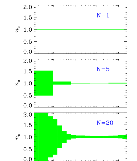
FIG. 1.: The precision with which the spectral indices in each bin can be measured, shown for three different numbers of bins ($N=1,5,20$), for the case where only the temperature anisotropy can be measured. Shown are the $1\sigma$ error bars around the central value which in all cases is $n_{s}=1$.

In Fig. 1 the precision with which $n_{s}(i)$ can be measured is shown for different numbers of bins, for the case where only the temperature power spectrum can be measured. Not surprisingly, the precision with which the effective spectral index in each bin can be measured depends strongly on the number of bins. For only one bin, $\Delta n_{s}/n_{s}=8.21\times 10^{-3}$, whereas for 20 bins, the smallest $\Delta n_{s}/n_{s}$ is $3.49\times 10^{-2}$. Thus, there is a trade-off between the resolution in $k$-space and the resolution in $n_{s}$. Detecting a low-amplitude narrow feature is not possible, whereas either a broad low-amplitude or a narrow high-amplitude feature should be detectable. In agreement with Wang, Spergel and Strauss [13, 14] we find that the CMBR data is most sensitive in the range $k\simeq 10^{-3}-10^{-1}{\rm Mpc}^{-1}$. If polarization can also be measured, the precision with which the $n_{s}(i)$ can be measured increases. Fig. 2 shows the same as Fig. 1, but with the inclusion of polarization. Indeed, the precision on the individual bin amplitudes increases by a large factor. For only one bin, $\Delta n_{s}/n_{s}=2.90\times 10^{-3}$, whereas for 20 bins, the smallest $\Delta n_{s}/n_{s}$ is now $9.49\times 10^{-3}$.

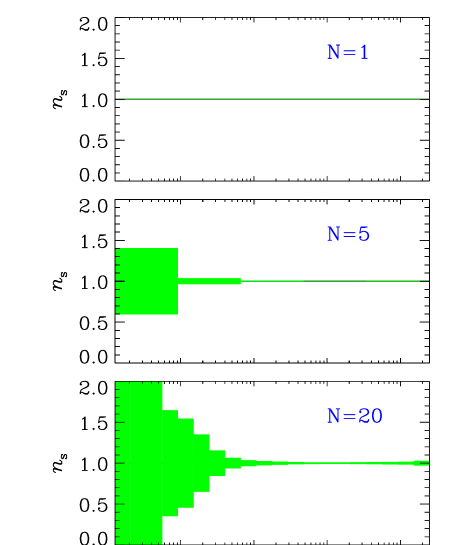
FIG. 2.: The precision with which the spectral indices in each bin can be measured, shown for three different numbers of bins ($N=1,5,20$), for the case where both temperature and polarization can be measured. Shown are the $1\sigma$ error bars around the central value which in all cases is $n_{s}=1$.

Next, a fundamental question is how much the ability to determine the other fundamental parameters depends on the number of bins in $k$-space. Figs. 3 and 4 show the precision in measuring the other cosmological parameters as a function of $N$, the number of bins. Fig. 2 is for the case where only the temperature anisotropy can be measured. For all the cosmological parameters, except $\tau$, there little degeneracy between these parameters and the power spectrum indices, meaning that there is little loss of ability to pin down these parameters. From $N=10$, the resolution begins to decrease, although quite slowly, and at $N=30$ it is for instance down by about 40% for $\Omega_{b}$. Clearly, the spectral indices, $n_{s}(i)$, are not very degenerate with the other cosmological parameters. The reason is that the discontinuous binning in the power spectrum is very hard to mimic by continuous changes in other parameters. This finding is in agreement with Ref. [13, 14], where such a binning was also used. However, there is a marked difference compared with the findings of Ref. [12]. In this work, smoothness of the power spectrum was enforced by using smooth shape functions peaked at a given point in $k$-space instead of discontinuous binning. These authors find that the uncertainty in the other parameters increases very rapidly with $N$, rising by more than a factor of 10 at $N=30$ [12]. However, using smooth functions to describe the power spectrum could indeed be expected to be able to mimic changes in other parameters to a much higher degree than our approach. So it is not surprising that a much higher degree of degeneracy is found. On the other hand, as will be seen in the next section, using a discontinuous binning has the very clear disadvantage that it can be difficult to achieve reasonable likelihood fits if the number of bins is too small.

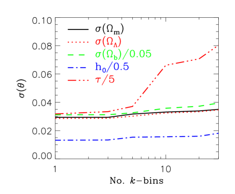
FIG. 3.: The precision with which the other cosmological parameters, $\Omega_{m},\Omega_{\Lambda},\Omega_{b}$ and $H_{0}$, measured as a function of the number of bins in $k$-space, for the case where only the temperature anisotropy can be measured. The precision is quantified in terms of the standard error, $\sigma$.

In line with this discussion, it was shown by Kinney [15] that smooth power spectrum features can mimic variations in the cosmological parameters almost exactly (to within cosmic variance). In this work 75 bins in $k$-space were used and the power spectrum smoothened by cubic spline interpolation, leading to a very large degree of degeneracy between the $k$-space power spectrum and the other cosmological parameters.

The one exception to the above is the optical depth to reionization, $\tau$. Here there is a very large degree of degeneracy, which increases rapidly with the number of bins. This effect was also described by Wang, Spergel and Strauss [13]. It happens because the effect of reionization is to suppress the amplitude at small scales by a factor $e^{-2\tau}$. This can be quite easily mimicked by suppressing the $k$-space power spectrum at small scales.

However, Fig. 4 shows the case where polarization can also be measured. In this case, the degeneracy between $\tau$ and the $k$-space spectrum is broken, and the ability to determine the value of $\tau$ is increased by a large factor. For the other cosmological parameters, the precision is also increased, but not as dramatically.

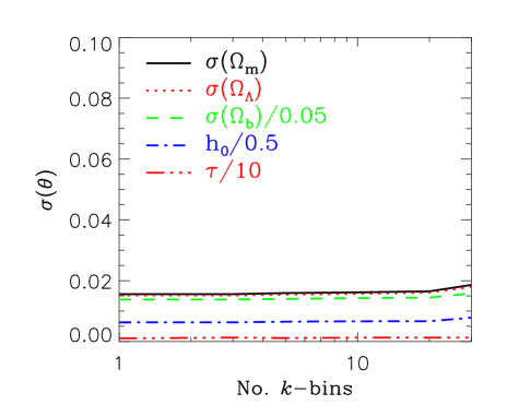
FIG. 4.: The precision with which the other cosmological parameters, $\Omega_{m},\Omega_{\Lambda},\Omega_{b}$ and $H_{0}$, measured as a function of the number of bins in $k$-space, for the case where both temperature and polarization can be measured. The precision is quantified in terms of the standard error, $\sigma$.

III Numerical Spectrum Reconstruction

Having done this initial estimate of how precisely the initial power spectrum can be estimated, it is important to see how such a power spectrum reconstruction works in practise. In order to investigate this, we have produced 10 synthetic spectra based on a underlying theoretical model. These spectra are calculated assuming Gaussian errors given by cosmic variance only. In order to simulate a possible feature in the power spectrum we introduce a Gaussian “bump”, so the spectral index has the form

$$n_{s}=1-A\exp\left(-\frac{(\log(k_{*})-\log(k_{0,*}))^{2}}{\alpha}\right),$$ (18)

where $k_{*}=k/1\,{\rm Mpc}^{-1}$. This bump is characterised by three parameters: $A$, the amplitude, $k_{0,*}$, the position in $k$-space, and $\alpha$, the width. For the underlying cosmological model we have chosen the same standard CDM model as in the last section, so the model parameters are: $\Omega=\Omega_{m}=1$, $\Omega_{b}=0.05$, $H_{0}=50\,\,{\rm km}\,{\rm s}^{-1}\,{\rm Mpc}^{-1}$, $A=0.7$, $\alpha=0.1$ and $\log k_{0,*}=-2$. Thus, the bump has been placed closed to the region where the CMBR data is most sensitive. Note that in this section we use only information related to the temperature power spectrum, not the polarisation spectrum.

On each of these synthetic spectra we try reconstructing the power spectrum using the logarithmic binning method introduced in the previous section. The likelihood optimization algorithm is based on the simulated annealing principle described in Ref. [21]. This method has the advantage that it is very fast for highly non-linear optimization over many-dimensional parameter spaces, exactly the problem that is faced here. In Fig. 3 we show the values extracted by the parameter reconstruction for three different numbers of bins, $N=5,10$ and 20.

In the $N=5$ case the individual bins are broader than the bump to be reconstructed. This shows up in the fact that no good fit is achieved ($\langle\chi^{2}_{\rm min}\rangle/{\rm d.o.f}=12.7$), and the spectrum reconstruction is quite poor. The reconstructed spectrum does show some evidence of a lower spectral index around the position of the bump, but the magnitude is not correct. For $N=10$ the reconstruction is already much better and reproduces the actual slope of the underlying spectrum. However, $\langle\chi^{2}_{\rm min}\rangle/{\rm d.o.f}=8.06$, so the fit is not very good in this case either. In the last case where $N=20$ the reconstructed spectrum again follows the underlying one reasonably well. However, at $N=20$ the uncertainty on the individual bin amplitudes is already significantly larger than for $N=10$. By going to an even higher number of individual bins, the spectrum bump will be smeared out beyond recognition. The $\chi^{2}$-fit is significantly better than for $N=10$ ($\langle\chi^{2}_{\rm min}\rangle/{\rm d.o.f}=2.84$), although far from what should be expected from a “good” fit ($\langle\chi^{2}_{\rm min}\rangle/{\rm d.o.f}\simeq 1$).

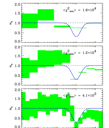
FIG. 5.: The reconstructed power spectrum from likelihood maximisation over 10 synthetic spectra. The boxes show the $1\sigma$ error intervals. The full line shows the underlying $k$-space power spectrum used to generate the synthetic spectra.

The reason for these very high $\chi^{2}$ values is that it is quite hard to mimic a smooth feature in the power spectrum with a sequence of discontinuous bins. Thus, even though it is indeed possible to map out the shape of the power spectrum, it is not possible to achieve a good fit in terms of the likelihood without letting $N\to{\rm d.o.f}$. However, going much beyond $N=20$ increases the uncertainty in the individual bin amplitudes and doing the likelihood maximization is already quite demanding numerically at $N=20$.

Finally, with a large number of bins (10 or 20) the reconstruction at scales smaller than the bump (large $k$) is consistently predicting a too low spectral index. This effect is worrying and to investigate whether it is a generic feature of any discontinuous binning method, or specific to our choice, where each bin has a “tilt”, $P(k)_{i}\propto k^{n_{s}(i)-1}$, we also do the reconstruction using the same method as Wang, Spergel and Strauss [13]. Here, the power in each bin is assumed to have constant amplitude over the entire bin so that $P(k)_{i}=A_{i}$. We show the reconstruction for the case of $N=20$ in Fig. 6. For this case, the reconstruction of the power spectrum bump is actually better than for the “tilt” spectrum reconstruction. There is no trace of the spuriously low spectral index found at high $k$. However, the $\chi^{2}$ is substantially worse for this method, with $\langle\chi^{2}_{\rm min}\rangle/{\rm d.o.f}=3.45$. From this, a robust conclusion is that for discontinuous binning the obtainable fits are quite poor in terms of $\chi^{2}$, regardless of the binning method. However, it is possible to detect features in the spectrum by this method. At least the tilted binning method can show spurious effects, so one should be careful about making strong conclusions without going through several different methods of spectrum reconstruction.

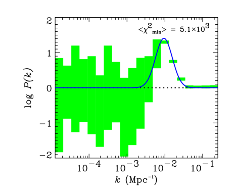
FIG. 6.: The reconstructed power spectrum from likelihood maximisation over 10 synthetic spectra, for the case of $N=20$. The boxes show the $1\sigma$ error intervals. The full line shows the underlying $k$-space power spectrum used to generate the synthetic spectra.

Just for comparison we have also done a spectrum reconstruction where the free parameters are those describing a smooth scale invariant power-law spectrum ($n_{s}=1$) with a Gaussian bump: $A,k_{0,*}$ and $\alpha$, instead of using $n_{s}(i)$. The values extracted from likelihood maximisation on the 10 synthetic spectra are given in Table I. Clearly, in this case, the true underlying spectrum is recovered to very good accuracy because the same functional form is used in the fit as in the underlying power spectrum. Also the $\chi^{2}$ values are completely consistent with what is expected from a good fit.

So using smooth fitting functions could have the advantage of being better able to fit smooth features in the underlying initial power spectrum. However, the discontinuous binning method has the advantage of being very model independent. So a possible way to proceed would be to initially try the discontinuous binning method, and only for refinements go to more complicated fitting functions.

IV Discussion

We have discussed the possibility for measuring the shape of the primordial power spectrum by using precision measurements of CMBR fluctuations. The method employed was to parametrise the spectrum as a power-law, binned in $k$-space. An analysis of the obtainable precision in measuring the power spectrum, using a Fisher matrix analysis, showed that it should be possible to detect features that are sufficiently broad by using CMBR observations.

However, there are some practical problems involved in this spectrum reconstruction. If the power spectrum is parametrised by binning it in $k$-space, it is very difficult to mimic any smooth features in the underlying power spectrum. Especially if the feature is comparable in width to the individual bins the reconstructed spectrum can show spurious features. Nevertheless, by going to a sufficiently fine binning it is possible to map out the general shape of the power spectrum, although still very difficult to get a good fit in terms of the likelihood.

The fact that it is possible to reconstruct the underlying $k$-space power spectrum from CMBR observations opens up the possibility of probing physics at the time of spectrum formation by observing the universe at CMBR formation ($T\sim 4000$K). As was for instance discussed in Refs. [23, 22], if the primordial fluctuations are produced during the inflationary epoch, it is possible to reconstruct the inflationary potential, $V(\phi)$, from the $k$-space spectrum.

However, in addition to that it will be possible to detect non-power-law features in the power spectrum using this discrete binning method. Such features are for instance predicted to occur in the multiple inflation model of Adams, Ross and Sarkar [11]. Here, the effect of symmetry breaking during the inflationary period was discussed. If such spontaneous symmetry breaking occurs along flat directions, short inflationary periods will result, leaving distinct non power-law features in the power spectrum. Another possible mechanism for producing features is the resonant production of particles during inflation discussed by Chung et al. [10].

Note that the CMBR is mainly sensitive to power spectrum at $k\simeq 10^{-3}-10^{-1}\,\,{\rm Mpc}^{-1}$. Any features outside this region in $k$-space would not be detectable, so the CMBR can at most probe a very small region of the inflationary period. However, as discussed for instance in Ref. [13, 14], by also using data from large scale structure (LSS) surveys such as the Sloan Digital Sky Survey it is possible to increase the region of $k$-space that can be probed. LSS surveys are sensitive to smaller scales than the CMBR (for instance the Sloan survey should probe the region $k\simeq 10^{-2}-1\,\,{\rm Mpc}^{-1}$), and by combining MAP/PLANCK with such surveys it should be possible to have sensitivity in the region $k\simeq 10^{-3}-1\,\,{\rm Mpc}^{-1}$. In addition to this, including data from large scale surveys can break some of the cosmological parameter degeneracies [7]. For instance, using CMBR data alone it is impossible to determine either $\Omega_{m}$ or $\Omega_{\Lambda}$ separately with high precision. The parameter that can be measured is the total energy density $\Omega=\Omega_{m}+\Omega_{\Lambda}$. However, the LSS surveys are sensitive to a different combination of $\Omega_{m}$ and $\Omega_{\Lambda}$, and by adding this information the degeneracy between them can be broken [7].

TABLE I.: The recovered parameters from the fit to a Gaussian bump overlayed on a scale invariant spectrum. 10 synthetic spectra were used for the reconstruction.

Parameter	found	expected
$\chi^{2}_{\rm min}$	$1516.7\pm 50.4$	$1496\pm 54.7$
$\alpha$	$0.1004\pm 0.0035$	0.1
$\log k_{0,*}$	$-2.0004\pm 0.0059$	$-2$
$A$	$0.6931\pm 0.003$	$0.7$