The Formation of Broad Line Clouds in the Accretion Shocks of Active Galactic Nuclei

Abstract

Recent work on the gas dynamics in the Galactic Center has improved our understanding of the accretion processes in galactic nuclei, particularly with regard to properties such as the specific angular momentum distribution, density, and temperature of the inflowing plasma. With the appropriate extrapolation of the physical conditions, this information can be valuable in trying to determine the origin of the Broad Line Region (BLR) in Active Galactic Nuclei (AGNs). In this paper, we explore various scenarios for the cloud formation based on the underlying principle that the source of plasma is ultimately that portion of the gas trapped by the central black hole from the interstellar medium. Based on what we know about the Galactic Center, it is likely that in highly dynamic environments such as this, the supply of matter is due mostly to stellar winds from the central cluster.

Winds accreting onto a central black hole are subjected to several disturbances capable of producing shocks, including a Bondi-Hoyle flow, stellar wind-wind collisions, and turbulence. Shocked gas is initially compressed and heated out of thermal equilibrium with the ambient radiation field; a cooling instability sets in as the gas is cooled via inverse-Compton and bremsstrahlung processes. If the cooling time is less than the dynamical flow time through the shock region, the gas may clump to form the clouds responsible for broad line emission seen in many AGN spectra. Clouds produced by this process display the correct range of densities and velocity fields seen in broad emission lines. Very importantly, the cloud distribution agrees with the results of reverberation studies, in which it is seen that the central line peak (due to infalling gas at large radii) responds slower to continuum changes than the line wings, which originate in the faster moving, circularized clouds at smaller radii.

1 INTRODUCTION

The spectra of many AGNs, including Seyfert galaxies and quasars, are distinguished by strong, broad emission lines, with a full width at half maximum intensity (FWHM) of $\sim 5000\ \mathrm{km\ s^{-1}}$, and a full width at zero intensity (FWZI) of $\sim 20,000\ \mathrm{km\ s^{-1}}$ (e.g., Peterson (1997)). From the observed strength of UV emission lines, we know that the temperature of the emitting plasma is on the order of a few times $10^{4}\ \mathrm{K}$ (e.g., Osterbrock (1989)), insufficient to produce the observed line widths via thermal (Doppler) broadening. Instead, bulk motions of the BLR gases appear to be responsible for the line broadening.

Because reverberation studies show a direct response of emission-line strengths to continuum variability (e.g., Clavel et al. (1991)), we know that the BLR gas must be photoionized by the continuum. The International AGN Watch consortium has carried out long-term optical and ultraviolet monitoring on a set of four Seyfert 1 galaxies: NGC 5548 (e.g., Korista et al. (1995); Peterson et al. (1999)), NGC 3783 (Reichert et al. (1994); Stirpe et al. (1994)), Fairall 9 (Rodríguez-Pascual et al. (1997); Santos-Lleó et al. (1997)), and NGC 7469 (Wanders et al. (1997); Collier et al. (1998)); and the broad line radio galaxy 3C 390.3 (Dietrich et al. (1998); O’Brien et al. (1998)). In all sources, it is observed that higher ionization lines respond faster than lower ionization lines. This would indicate that the former are found at smaller radii using a simple $r\sim c\,\tau_{delay}$ argument. The response time for the same line varies by source, even when the luminosities are very similar, indicating that the simple $r_{\mathrm{BLR}}\propto L^{1/2}$ rule alone does not determine the size of the BLR. Indeed, other factors, such as geometry, viewing angle, and spectral energy distribution (SED) may play equally important roles in determining its volume (e.g., Robinson (1995); Wandel (1997)).

What the reverberation studies do tell us, however, is that the size of the BLR ranges from a few to several hundred light days, with a radial dependence on ionization state and possibly other physical properties. It is also seen that the response delay within a given source tends to increase with increasing luminosity (Peterson et al. (1999)), consistent with the $r_{\mathrm{BLR}}\propto\mathit{L^{1/2}}$ rule. The optical continuum displays little or no lag ($\tau_{delay}\lesssim 2$ days) in variability with respect to the ultraviolet continuum, and the amplitude of variations are typically weaker at longer wavelengths (Collier et al. (1998)).

The ionization parameter, $U\equiv n_{\gamma}/n$, which is the ratio of the number density of hydrogen ionizing photons $n_{\gamma}$ to the number density of hydrogen nuclei $n$, determines the physical state of the BLR plasma. In modeling the BLR with photoionization simulations, it is observed that a value of $10^{-2}<U<1$ (e.g., Netzer (1990)) is required to reproduce the correct line strength and ionization state of the gas. Because of the radial structure of the BLR, it is likely that the density of emitting gas varies with radius, within the range $10^{8}\ {\mathrm{c}m}^{-3}\lesssim n\lesssim 10^{11}\ {\mathrm{cm}^{-3}}$ (e.g., Peterson (1997)). However, Marziani et al. (1996) find that the BLR may extend to even higher densities ($n_{e}\sim 10^{12.5}\;\mathrm{cm}^{-3}$). In addition, the BLR may contain a mixture of optically thick and thin gases. Optically thick gas must be present to account for the variability of the low ionization Mg II, Ly$\alpha$, and Balmer lines (e.g., Ferland et al. (1992)). Optically thin gas, on the other hand, may account for the Baldwin effect, a negative correlation between the ultraviolet emission-line equivalent width and continuum luminosity; and the Wamsteker-Colina effect, a negative correlation between C IV $\lambda 1549$/Ly$\alpha$ ratio and continuum luminosity (Shields, Ferland & Peterson (1995)). Green (1995), however, suggests that these effects are due to changes in the SED with luminosity. The set of other important observational constraints include (i) the absence of a deep Ly$\alpha$ absorption edge in AGN spectra indicates that the BLR gas must cover only a small fraction (5 - 25%) of the continuum source (e.g., Bottorff et al. (1997)), and (ii) the observed line strength to continuum ratio requires a small volume filling factor ($\sim 10^{-7}$; Netzer (1990)).

The recent work in modeling (and observations of) the BLR suggests that the clouds are spread over a wide range of radii and may display a wide range of particle density, $n_{c}$, at each radius. The emission from each cloud can be determined largely from the ionization parameter $U$. An important result of this “locally optimally emitting cloud” model is that the predicted integrated spectrum from all clouds depends only weakly on the parameters, including the SED, column density of the clouds, and the cloud distribution as a function of radius (Baldwin (1997)). However, the spectrum does depend strongly on $n_{c}$ and on the elemental abundances. A consequence of the weak dependence on many of the input parameters is that several different models may be able to account for at least some of the observed spectra.

1.1 A Sample of Current Models

There are several models in the literature that account for the origin and nature of the BLR. For example, Emmering, Blandford, & Shlosman (1992) propose that the BLR is associated with magnetohydrodynamic winds originating in a dusty molecular accretion disk. Dense molecular clouds are loaded onto magnetic lines threading the disk and are centrifugally accelerated outward. Being exposed to the central continuum, these clouds are quickly photoionized and produce the observed emission lines. This model correctly “postdicts” both the observed shape and differential response time of the C IV $\lambda 1549$ line, with its mid-red wing portion responding fastest to continuum variations (Bottorff et al. (1997)).

In a different model, Murray et al. (1995) propose that the broad absorption lines (BALs) seen in $\sim 10\%$ of radio quiet QSOs are produced in outwardly flowing radiation- and gas-pressure driven winds rising from an accretion disk. These winds would also be partially responsible for the broad line emission. As this model requires shielding of the absorbing gas from soft X-rays, the absence of BALs in radio-loud quasars and Seyfert galaxies is explained by the fact that these objects are strong X-ray emitters (Murray & Chiang (1995)). Cassidy & Raine (1996) present a similar model in which BLR clouds form as the result of the interaction of an outflowing wind with the surface of an accretion disk.

Alexander & Netzer (1994) propose that the AGN broad-line emission originates in the winds or envelopes of bloated stars in the nuclear environment. They obtain good agreement with the line ratios and response features seen in AGNs, but they encounter some difficulty in reproducing the broad line wings (Alexander & Netzer (1997)).

Finally, Perry & Dyson (1985) propose that the BLR clouds are formed as the result of a cooling instability that occurs when an outflowing wind from the black hole encounters an “astrophysical obstacle” and is shocked. Rapid cooling in the shocked gas causes the plasma to clump into clouds, and the observed line widths are then due to cloud acceleration along the shocks.

1.2 The Analogy with the Galacic Center

In this paper, we will take the approach that it may be worthwhile in formulating a model for the BLR to seek guidance from the galactic nucleus we know best—that of our own Galaxy. The evidence for the presence of a supermassive black hole, coincident with the radio source Sgr A* at the Galactic Center, is now the most compelling of any such systems (for a recent review dealing mostly with the observational characteristics of this region, see Mezger, Duschl & Zylka 1996; for a summary of the theoretical status concerning Sgr A*, see Melia 1998). The motions of stars within 1 pc of Sgr A* seem to require a central dark mass of $(2.61\pm 0.35)\times 10^{6}\;M_{\odot}$ (Genzel et al. 1997; Ghez et al. 1998), in good agreement with earlier ionized gas kinematics and velocity dispersion measurements.

Our proximity to the Galactic Center provides us with the rather unique opportunity of examining the gas dynamics surrounding such a massive point-like object with unprecedented detail. Combined with multi-dimensional hydrodynamical simulations, this extensive body of multi-wavelength data is opening our view into the complex patterns of plasma-plasma and plasma-stellar interactions. It is likely that many of Sgr A*’s characteristics are associated with the liberation of gravitational energy as gas from the ambient medium falls into a central potential well (Melia 1994; Ruffert & Melia 1994). There is ample observational evidence in this region for the existence of rather strong winds in and around Sgr A* itself (from which the latter is accreting), e.g., the cluster of mass-losing, blue, luminous stars comprising the IRS 16 assemblage located within several arcseconds from the nucleus. Measurements of high outflow velocities associated with IR sources in Sgr A West (Krabbe et al. 1991) and in IRS 16 (Geballe et al. 1991), the $H_{2}$ emission in the circumnuclear disk (CND) from molecular gas being shocked by a nuclear mass outflow (Genzel et al. 1996; but see Jackson et al. 1993 for the potential importance of UV photodissociation in promoting this $H_{2}$ emission), broad Br$\alpha$, Br$\gamma$ and He I emission lines from the vicinity of IRS 16 (Hall et al. 1982; Allen et al. 1990), and radio continuum observations of IRS 7 (Yusef-Zadeh & Melia 1992), provide clear evidence of a hypersonic wind, with a velocity $v_{w}\sim 500-1000$ km s^-1, a number density $n_{w}\sim 10^{3-4}$ cm^-3, and a total mass loss rate $\dot{M}_{w}\sim 3-4\times 10^{-3}\;M_{\odot}\ {\mathrm{y}r^{-1}}$, pervading the inner parsec of the Galaxy.

In recent years, several studies have addressed the question of what the physical state of this gas is likely to be as it descends into the deepening gravitational potential well of the massive black hole. In the classical Bondi-Hoyle (BH) scenario (Bondi & Hoyle 1944), the mass accretion rate for a uniform hypersonic flow is $\dot{M}=\pi{R_{A}}^{2}m_{H}n_{w}v_{w}$, in terms of the accretion radius $R_{A}\equiv 2GM/{v_{w}}^{2}$. With the conditions at the Galactic Center (see above), we would therefore expect an accretion rate $\dot{M}\sim 10^{22}{\rm\,g\,s^{-1}}$ onto the black hole, with a capture radius $R_{A}\sim 0.02{\rm\,pc}$.

In reality the flow past the supermassive black hole is not likely to be uniform, so this value of $\dot{M}$ may be greatly underestimated. For example, one might expect many shocks to form as a result of wind-wind collisions within the cluster of wind producing stars, even before the plasma reaches $R_{A}$. With this consequent loss of bulk kinetic energy, it would not be surprising to see the black hole accrete at an even larger rate than in the uniform case. The implications for the gas dynamics in the region surrounding the black hole are significant. Coker & Melia (1997) have undertaken the task of simulating the BH accretion from the spherical winds of a distribution of 10 individual point sources located at an average distance of a few $R_{A}$ from the central object. The results of these simulations show that the accretion rate depends not only on the distance of the mass-losing star cluster from the accretor but also on the relative spatial distribution of the sources.

These calculations indicate that to fully appreciate the morphology of the gaseous environment surrounding the accretor, one must pay particular attention to the spatial distribution of specific angular momentum $l$ in the accreting gas. Written as $l\equiv\lambda cR_{S}$, where $R_{S}\equiv 2GM/c^{2}$ is the Schwarzschild radius, the accreted $\lambda$ can vary by $50\%$ over $\lower 2.15277pt\hbox{$\;\buildrel<\over{\sim}\;$}200$ years with an average equilibrium value of $10-50$ for the conditions in the Galactic Center. This is interesting in view of the fact that earlier simulations based on a uniform flow—the “classic” Bondi-Hoyle accretion, producing a bow shock—resulted in $\langle\lambda\rangle\sim 3-20$. It appears that even with a large amount of angular momentum present in the wind, relatively little specific angular momentum is actually accreted. This is understandable since clumps of gas with a high specific angular momentum do not penetrate to within $1\ R_{A}$. The variability in the sign of the components of $\lambda$ suggests that if an accretion disk forms at all, it dissolves and reforms (perhaps) with a different sense of spin on a time scale of $\sim 100$ years (Coker & Melia (1997)).

The fact that AGNs are significantly more gas rich and display a more powerful array of phenomena than the Galactic Center could mean that these ideas derived from the latter may not be valid in the case of the former. But one area where this type of gas morphology would certainly have a significant impact is in the structure and nature of the BLR. Our intention in this paper is therefore to frame our investigation of the BLR in AGNs with the conditions (i.e., clumping, distribution in specific angular momentum $\lambda$, density and temperature) we now believe to be prevalent in the Galactic nucleus, though scaled accordingly.

2 OVERVIEW OF THE MODEL

2.1 An Accretion Shock Scenario for the Production of BLR Clouds

We suggest that many of the observed properties of the BLR can be explained by a simple picture of cloud production within the accretion shocks surrounding the central black hole. For this, we shall adopt several of the ideas introduced in Perry & Dyson (1985, hereafter PD85) for the formation of clouds from cooling instabilities in these regions. In their model, a hypersonic, outflowing wind is incident upon a supernova remnant or other astrophysical obstacles, causing bow shocks to form around them. The shocked gas is compressed and heated, and is brought out of thermal equilibrium with the radiation field.

The equilibrium temperature $T_{eq}$ of a gas whose heating/cooling is dominated by radiative processes is determined by another ionization parameter (Krolik, McKee, & Tarter (1981))

$$\Xi\equiv\frac{F_{ion}}{nkTc}\;,$$ (1)

where $F_{ion}$ is the ionizing flux between 1 and $10^{3}$ ryd; then, $T_{eq}=T_{eq}(\Xi)$. Because the shock temperature $T_{s}\gg T_{eq}$, the shocked gas will rapidly cool via inverse-Compton and bremsstrahlung processes. If the cooling time is shorter than the dynamical time for the gas to flow along the shock, the cooled gas will clump and form clouds, which then stream along and behind the shock.

An important parameter in determining $T_{eq}$ is the Compton temperature $T_{C}$, at which Compton heating and cooling processes balance (e.g., Krolik, McKee, & Tarter (1981); Guilbert (1986)). The Compton temperature is highly sensitive to the shape of the continuum, particularly at high (X-ray and gamma ray) energies; typical AGN spectra have $T_{7}\approx 0.01-5$ (Mathews & Ferland (1987)), where $T_{7}\equiv T_{C}/(10^{7}\ {\mathrm{K}})$ . For these high values of $T_{C}$, we can state a couple of generalities about $T_{eq}$: if $\Xi\gg 1$, Compton processes dominate, and $T_{eq}\simeq T_{C}$; if $\Xi\ll 1$, collisional (bremsstrahlung) and recombination-line cooling dominate, and $T_{eq}\simeq 1-3\times 10^{4}$ K.

In our picture, we assume that gravitation dominates over the outward radiation pressure within the BLR (either because the outward radiation field is sub-Eddington, or because the radiative emission is anisotropic), allowing a hypersonic, accreting wind to feed the central black hole. In the AGN context, we re-examine the PD85 result for stellar wind bow shocks, and extend the idea of “astrophysical obstacles” to include Bondi-Hoyle accretion shocks and density perturbations due to wind-wind collisions and turbulence in the accretion flow. As discussed above, this is motivated by the recent simulations of the highly variable gas flows at the Galactic Center.

2.2 Model Parameters

Our model requires the specification of several parameters, including the density, velocity, and temperature profiles of the accreting wind as functions of radius, as well as the intensity and Compton temperature of the continuum. In order to keep our arguments general, we choose to model the wind flow using simple dimensional requirements. We adopt the view that the accreting gas circularizes before it reaches the event horizon, thereby forming a disk at small radii. The existence of an accretion disk in AGNs is inferred from, e.g., the axisymmetry observed in many sources (Brotherton (1996); Glenn, Schmidt, & Foltz (1994)). Again writing the specific angular momentum as $l\equiv\lambda cR_{S}$, it is easy to show that the circularization radius is

$$r_{circ}=2\lambda^{2}R_{S}\ .$$ (2)

If the central object dominates the gravitational potential, then the characteristic wind velocity scales as the free-fall velocity, $v_{w}(r)\approx v_{ff}=\sqrt{2GM/r}$. Due to mass conservation (which in the outer region gives $\dot{M}=4\pi r^{2}n_{w}v_{w}$) and assuming that the bolometric luminosity is related to the mass accretion rate by

$$L_{bol}=\epsilon\dot{M}c^{2}\ ,$$ (3)

where $\epsilon<1$ is the accretion efficiency, the wind density can be expressed as

$$n_{w}(r)=\frac{L_{bol}}{4\pi\,\sqrt{2GM}\,\epsilon\,m_{H}\,c^{2}\,r^{3/2}}\ .$$ (4)

The temperature $T_{w}$ of the gas undergoing steady, spherical infall is described by the Equation (Mathews & Ferland (1987))

$$\frac{dT_{w}}{dr}=-\frac{T_{w}}{r}+\frac{F_{c}(T_{w})}{v_{w}}\;,$$ (5)

which we use as an approximation for our non-steady flow. In Equation (5), the first term represents compressional heating and the second term is due to radiative heating/cooling, for which $F_{c}(T)$ is the cooling function of the gas (c.f., Eq. (A2) in the Appendix). As we are mainly concerned with establishing a minimum temperature of the flow, we have neglected the effects of viscosity, shocks, and the dissipation of magnetic energy, all of which may raise the value of $T_{w}$.

In a recent study, Wandel, Peterson and Malkan (1999) used reverberation data to infer central masses of $M_{8}\approx 0.02-4$ (where $M_{8}\equiv M/(10^{8}\ M_{\odot})$) for a sample of 17 Seyfert 1 galaxies and 2 quasars. They also determined a mass – monochromatic luminosity relation of $L(5100\ {\rm\AA})\simeq 10^{44}\,M_{8}^{1.25}\ \mathrm{erg\ s^{-1}}$ for these objects. Setting $L_{bol}=f_{bol}L(5100\ {\rm\AA})$ for the monochromatic – bolometric luminosity relation, with $f_{bol}=10$ consistent with the findings of Bechtold et al. (1987), we obtain

$$L_{bol}=10^{45}M_{8}^{1.25}\ \mathrm{erg\ s^{-1}}\ .$$ (6)

For the ionizing luminosity, we set $L_{ion}=f_{ion}L(5100\ {\rm\AA})$, where $f_{ion}=2.5$ has been chosen as a fiducial value. Under these assumptions, the only free parameters in the model are $M$, $\epsilon$, $T_{C}$, and $\lambda$.

2.3 Optical Depth of the Flow

The observed absence of the Fe K-shell edge in most AGN spectra indicates that the inter-cloud medium must be optically thin to X-radiation (e.g., Mathews & Ferland (1987)). This limit is written as $\tau_{K}<1$, where

$$\tau_{K}=\int_{r_{circ}}^{\infty}\delta_{Fe}\ \sigma_{K}n_{w}(r)\,dr$$ (7)

is the Fe K-shell optical depth, $\sigma_{K}=2.3\times 10^{-20}\ \mathrm{cm^{2}}$ is the total K-shell cross section (e.g., Morrison & McCammon (1983)), and $\delta_{Fe}$ is the elemental abundance of iron. Assuming that $\delta_{Fe}=3.3\times 10^{-5}$ (corresponding to the local ISM value; Dalgarno & Layzer (1987)) and that all Fe ions in the flow retain at least two electrons (a conservative estimate given the likely high temperature of the gas), then the condition for the flow to remain optically thin to X-radiation is

$$\lambda\gtrsim\frac{0.03\ M_{8}^{0.25}}{\epsilon}\;.$$ (8)

This follows from the use of Equations (3), (4), (6) and (7), with the appropriate definition of $r_{circ}$ in Equation (2). It is clear that this condition is met for reasonable values of $\epsilon$ and $\lambda$ (c.f., Sec. 1.2). Because $\delta_{Fe}\sigma_{K}\approx\sigma_{T}$, the flow will then also be optically thin to Compton scattering.

2.4 Cloud Formation

In order for clouds to form, the cooling time, $t_{cool}$, of the shocked gas must be less than the dynamical time, $t_{dyn}$, for the gas to be transported through the shock region; i.e., $t_{cool}<t_{dyn}$. The cooling time can be calculated numerically (c.f. Eq. A1 of the Appendix) if the initial temperature of the shocked gas is known. Assuming that the shock converts the ordered velocity of the flow into random (thermal) motions, the initial temperature should be $T_{s}\approx m_{H}\Delta(v^{2})/3k$, where $\Delta(v^{2})$ is the change in the square of the velocity across the shock.

We assume that the pre-shock conditions are those of the wind; i.e., $n_{w}$ and $v_{w}$ are used as the pre-shock density and velocity, respectively. At a strong shock, we have

$$v_{s}^{(n)}=v_{w}^{(n)}/4\;,\qquad v_{s}^{(t)}=v_{w}^{(t)}\;,\qquad n_{s}v_{s}^{(n)}=n_{w}v_{w}^{(n)}\;,$$ (9)

where the superscripts $(n)$ and $(t)$ refer to the normal and tangential velocity components, respectively, relative to the shock front and $v_{s}$ is the velocity of the shocked gas. In bow shocks, most of the kinetic energy of the incident flow is dissipated, so $\Delta(v^{2})\simeq v_{w}^{2}$. For shocks between obliquely incident gas flows, it is the component of the wind velocity normal to the shock that is converted into thermal energy, so $\Delta(v^{2})\simeq v_{w}^{(n)\,2}$.

2.5 Physical Properties of the Cooled Gas

As the shocked gas cools, it clumps to form clouds. Their physical characteristics, such as the number density $n_{c}$, the ionization parameter $U$, and the column depth $N_{H}$ through each clump, all contribute to a determination of the line emissivity using photoionization codes such as CLOUDY (Ferland (1996)). Assuming isobaric cooling occurs, the density of the cooled gas is

$$n_{c}=\left(\frac{T_{s}}{T_{eq}}\right)n_{s}\;.$$ (10)

The ionization parameter, $U$, is then determined directly from the luminous ionizing flux, the SED, and $n_{c}$. Finally, the column density of a cloud is given by $N_{H}\simeq n_{c}\;l_{c}$, where $l_{c}$ is the cloud size.

In the PD85 model, the maximum cloud size is set by the coherence length, $l_{coherence}\leq t_{cool}\ c_{s}$, where $c_{s}$ is the sound speed in the shocked gas. If the cooling is isobaric and steady, $l_{c}=\left(T_{eq}/T_{s}\right)^{1/3}l_{coherence}$. It seems that this model is overly optimistic, however, as turbulent mixing is likely to be very important in any shock. Random motions of the turbulent fluid will disrupt coherence within the cooling gas; the maximum cloud size is then dictated by the smallest scale at which turbulence persists. Unfortunately, this scale is not specified by our simple model, so $N_{H}$ remains relatively undetermined.

2.6 Cloud Confinement

Krolik, McKee, & Tartar (1981) first proposed the co-existence of cool, dense clouds (the source of the broad emission lines) confined by a hot, rarefied medium. They showed that it was possible, under the right spectral conditions, to have the two phases in pressure equilibrium (i.e., to have the same value of $\Xi$) and yet have vastly different temperatures. Unfortunately, two stable states can only co-exist in very hard AGN spectra, with $T_{C}\gtrsim 10^{8}$ K. Most AGN spectra are much softer than this, effectively ruling out the two-phase pressure equilibrium condition (Fabian et al. (1986)). Dense clouds emerging from the high-pressure shock environment will rapidly expand into the ambient flow at their sound speed (e.g., Reynolds & Fabian (1995)). Therefore, unless some other confinement mechanism is introduced, such as a magnetic field (e.g., Emmering, Blandford, & Shlosman (1992)), the clouds produced within a shock are likely to survive only within the shock itself. As a result, the cloud motions are dictated by the shock motions, which are in turn dictated by the wind flow.

3 RESULTS

The condition for cooling, i.e., $t_{cool}<t_{dyn}$, sets a minimum length scale for the shock region. Shocked gas in regions smaller than this size will simply flow out of the region before it has time to cool. From the discussion in Sec. 2.4, we note that the dynamical time can be expressed as $t_{dyn}\approx d_{s}/v_{s}^{(n)}$, where $d_{s}$ is the size of the shock region. Our requirement for the minimum shock size is therefore

$$d_{s}>v_{s}^{(n)}\ t_{cool}\ .$$ (11)

In Figures 1 and 2, we plot the minimum value of $d_{s}$ for a range of values in the parameters $M$, $\epsilon$, and $T_{C}$. We have here set $v_{s}^{(n)}=v_{w}/4$, an upper limit that occurs when the colliding winds are incident normally. Our $d_{s}^{(min)}$ estimates are therefore rather conservative; for obliquely incident winds, smaller shock regions may suffice. It is reasonable to assume that shocks are possible sites for cloud formation only if $d_{s}^{(min)}\leq r$.

Figure 1 illustrates the effect of varying the central mass $M$ (left) and accretion efficiency $\epsilon$ (right). Increasing $M$ has the effect of decreasing $d_{s}^{(min)}$ at any given radius, thereby extending the plausible cloud production region to larger radii. This is because both the luminosity (via Eq. 6) and wind density (via Eq. 3) increase with $M$. With Compton cooling being proportional to the luminosity, and bremsstrahlung cooling (per particle) being proportional to the density (c.f. Eq. A2), the value of $t_{cool}$ becomes smaller. Decreasing the value of $\epsilon$ also decreases $t_{cool}$; smaller values of $\epsilon$ mean higher values of $n_{w}$ for any given luminosity (Eq. 3), thereby enhancing the bremsstrahlung cooling rate.

Figure 2 shows the effect of varying the Compton equilibrium temperature $T_{C}$. Plotted are the $d_{s}^{(min)}$ curves for $T_{7}=0.1$ and $1$ with fixed $M$ and $\epsilon$. There is no great difference between the cooling times, with the cooling occuring slightly faster in the case of the softer continuum spectrum. Note that cooling to $T\sim 10^{4}$ K does not occur for $T_{7}=10$. When the temperature of the cooling gas drops below $T_{C}$, the Compton heating/cooling term in Eq. (A2) changes sign; in order for cooling to continue, the bremsstrahlung term must dominate at $T\lesssim T_{C}$. In the high $T_{C}$ case, the gas has not cooled sufficiently for the (density-dependent) bremsstahlung term to dominate, so the gas simply equilibrates at $T_{eq}\simeq T_{C}$.

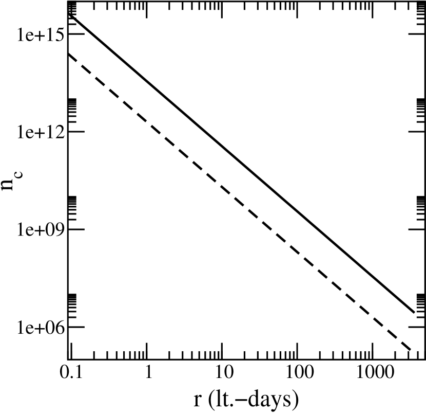
Figure 3: Density of shock-produced clouds. Solid: $M_{8}=1$; $\epsilon=0.1$ and $0.01$; $T_{7}=1$. Dashed: $M_{8}=0.1$; $\epsilon=0.1$ and $0.01$; $T_{7}=1$.

In Figure 3, we plot the density of the cooled (cloud) gas for a range of parameter values. Note that the gas displays the range in densities over radii inferred for the BLR. We find that the density at any given radius increases with $M$, but is insensitive to the values of $\epsilon$ and $T_{C}$. Note also that the density increases with decreasing $r$; this is consistent with the results of modeling the BLR using photoionization codes (e.g., Kaspi & Netzer (1999)).

4 MODELS OF SHOCK-FORMED CLOUDS

4.1 Stellar Wind Bow Shock Model

We next study a sample of shock producing mechanisms with the goal of determining plausible shock sites for cloud production. Let us begin by first considering the PD85 model, but now with an inflow (due to the accretion of ambient gas onto the central engine) to act as the agent of interaction with the winds from stars embedded within (although not co-moving with) this plasma; this is in contrast with the outflow assumed by these authors. In this picture, broad line clouds are produced within the bow shocks surrounding the stellar wind sources.

In this case, the size of the shock is determined by the stand-off distance (Perry & Dyson (1985)), which gives

$$d_{s}^{(sw)}\simeq 3.1\times 10^{29}\left(\frac{\dot{E}_{36}}{n_{w}v_{w}^{2}v_{o}}\right)^{1/2}\ \ {\rm[cm]}\;,$$ (12)

where $\dot{E}_{36}$ is the kinetic energy outflow rate in the stellar wind in units of $10^{36}\;\mathrm{erg}\;{\mathrm{s}}^{-1}$ and $v_{o}$ is the outflow velocity.

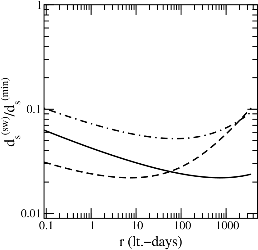
Figure 4: Ratio of stellar wind shock size to minimum shock length scale required for radiative cooling to form clouds. Solid: $M_{8}=1$, $\epsilon=0.1$, $T_{7}=1$. Dashed: $M_{8}=1$, $\epsilon=0.01$, $T_{7}=1$. Dot-dashed: $M_{8}=10$, $\epsilon=0.1$, $T_{7}=1$.

In Figure 4, we plot $d_{s}^{(sw)}/d_{s}^{(min)}$ using the fiducial values $v_{o}\approx 2,000\;\mathrm{km}\;{\mathrm{s}}^{-1}$ and $\dot{E}_{36}\approx 100$, typical for W-R stars (although these are probably upper limits for a typical stellar population). It can be seen that the size of these shocks is probably too small for these to be viable sites for cloud production via radiative cooling, thus confirming the PD85 result.

4.2 Bondi-Hoyle Accretion Shock Model

In the Bondi-Hoyle accretion process, a bow shock forms around the black hole when it accretes from a rather uniform, laminar flow. The length scale of the shock is roughly the accretion radius itself, i.e., $d_{s}^{(BH)}\approx(0.1-1)\,R_{A}\simeq(0.1-1)\,r$ (see Sec. 1.2). We have already seen in Figs. (1) and (2) that the requirement $d_{s}^{(min)}<r$ can be met for a wide variety of parameters over the range of relevant radii. Therefore, Bondi-Hoyle shocks around the central mass concentration are plausible sites for cloud production.

However, it should be noted that $R_{A}$ is unlikely to remain the only relevant scale as a Bondi-Hoyle shock is likely to break up into smaller scale shocks in a realistic (unsteady) flow. This would have the effect of reducing $t_{dyn}$. Production of BLR clouds by this mechanism is therefore dependent on the stability of the large scale shock structure.

An important signature of the highly ordered flow around a Bondi-Hoyle shock would be a rather narrow line emission profile whose overall redshift is dependent on viewing angle. This is because the clouds flowing along a shock have roughly parallel velocities. In addition, the Bondi-Hoyle shock does not provide a sufficiently broad distribution of cloud properties inferred for an extended BLR. It is therefore unlikely that a single Bondi-Hoyle accretion shock could produce the broad line profiles seen in AGN spectra.

4.3 Wind Collision and Turbulent Accretion Shock Model

The final source of BLR clouds we consider here is shocks produced by large-scale wind collisions and turbulence within the overall flow. The motivation for this is that realistic 3D simulations of the accretion onto a massive nucleus from a distribution of wind sources (Coker & Melia 1997) indicate that a single Bondi-Hoyle bow shock is difficult to form or maitain. Instead, the stellar wind-wind collisions produce an array of shock segments and a consequent turbulent inflow towards the black hole. In this picture, clouds are produced continually throughout the extended BLR, so we avoid the problem of having to confine long-lived clouds; instead clouds that evaporate upon leaving the shock region are continually replaced by newly formed clouds at other locations within the inflow.

The shock regions must be large to allow cooling to occur (c.f., Figs. 1 and 2), but these are readily obtainable for a realistic flow. Because the shocks, and therefore the clouds themselves, are embedded within the overall accretion pattern, the velocity of the clouds is roughly equal to that of the captured wind; i.e., $v_{c}\simeq v_{w}$. Clouds that move at nontrivial velocities relative to the surrounding medium are subjected to disruption via Rayleigh-Taylor instabilities (Mathews & Ferland (1987)). The winds, and therefore the clouds, display a $v(r)\propto r^{-1/2}$ velocity field fully consistent with, e.g., the Peterson & Wandel (1999) conclusion that the BLR velocity fields in NGC 5548 mimic Keplerian motions about a single central mass. Assuming that a large number of shocks exist at different locations within the flow, it should be possible to reproduce the observed line profiles. We have found it quite straightforward to do this within the context of this model. However, since the actual profile depends on the number and location of the shocks, which are not known a priori, an actual fitting such as this is not yet warranted.

5 CONCLUSIONS

In this paper, we have considered a broad range of possible gas configurations in a wind accreting onto the central black hole, with physical conditions that may produce BLR clouds via cooling instabilities within shocks. We note that in order to reproduce the observed line shape in actual sources, the BLR clouds cannot all be produced within a single outer region such as a Bondi-Hoyle shock, since this does not account for the required range in cloud properties at smaller radii. Instead, we have found that the best scenario involves local cloud production throughout the overall accretion flow. We conclude that a viable model for the formation of the BLR is one in which ambient gas surrounding the black hole (e.g., from stellar winds) is captured gravitationally and begins its infall with a (specific angular momentum) $\lambda$ representative of a flow produced by many wind-wind collisions and turbulence rather than a smooth Bondi-Hoyle bow shock. In this process, the gas eventually circularizes at $r_{circ}\approx 2\lambda^{2}R_{S}$, but by that time all of the BLR clouds have been produced, since at that radius the gas presumably settles onto a planar disk. As such, this picture is distinctly different from models in which the clouds are produced within a disk and are then accelerated outwards by such means as radiation pressure or magnetic stresses.

We note that these results are consistent with current reverberation studies. In our model, the inner radius of the BLR is determined by the circularization radius. Our model predicts that $r_{circ}\approx 2\,\lambda_{10}^{2}\,M_{8}$ lt.-days, where $\lambda_{10}\equiv\lambda/10$, which is consistent with the inferred inner BLR radius of a few light days. This scenario is also consistent with the differential line response seen in most sources (e.g., Korista et al. (1995)), with the blue and red wings responding fastest to continuum changes before the central peak. Our picture of the BLR has the broad wings formed by rapidly moving gas at small radii and the central peak formed by slower moving gas at larger radii.

Finally, we consider the argument that broad line emission cannot be produced by discrete clouds (Arav et al. (1998)). This reasoning is based on the assumption that each cloud has a fixed set of parameters, such as density, thickness, velocity, etc. In our model, with the clouds continually forming in regions of high turbulence, each cloud region can display a wide range of properties. Therefore, we suggest that the cross-correlations that appear with fixed cloud properties would vanish. Given the viability of this picture, it now remains to be seen whether the vast array of BLR phenomena observed in sources ranging from Seyferts to high redshift quasars can be self-consistently accounted for with this single description. This is work in progress and the results will be reported elsewhere.

6 ACKNOWLEDGEMENTS

The authors would like to thank Amri Wandel for his helpful review. This work was supported by an NSF Graduate Fellowship at the University of Arizona, by a Sir Thomas Lyle Fellowship and a Miegunyah Fellowship for distinguished overseas visitors at the University of Melbourne, and by NASA grant NAG58239.

Appendix A Calculation of the Cooling Time Scale

Following Krolik, McKee, & Tartar (1981) and Perry & Dyson (1985), we calculate the cooling time scale for a shocked gas to cool from an initial temperature, $T_{i}$, to the equilibrium temperature, $T_{f}$, using the expression

$$t_{cool}=\int_{T_{f}}^{T_{i}}\frac{dT}{F_{c}(T)}\;,$$ (A1)

where $F_{c}(T)$ is the net cooling rate. From Matthews & Ferland (1987), we have that

$$F_{c}(T)=\frac{4\sigma_{T}}{3m_{e}c^{2}}\frac{L_{bol}}{4\pi r^{2}}(T-T_{C})+\frac{n\lambda_{B}T^{1/2}}{3k}\;.$$ (A2)

The first term is due to Compton heating/cooling processes, and the second term is due to bremsstrahlung (free-free) emission.

Equation (A2) is valid for $T\gtrsim 10^{5}\ \rm K$. Below this temperature, collisional and radiative transitions in the plasma cause very rapid cooling. Therefore, $T_{f}=10^{5}\ \rm K$ is taken as the lower limit of integration for the cooling processes described in this paper.

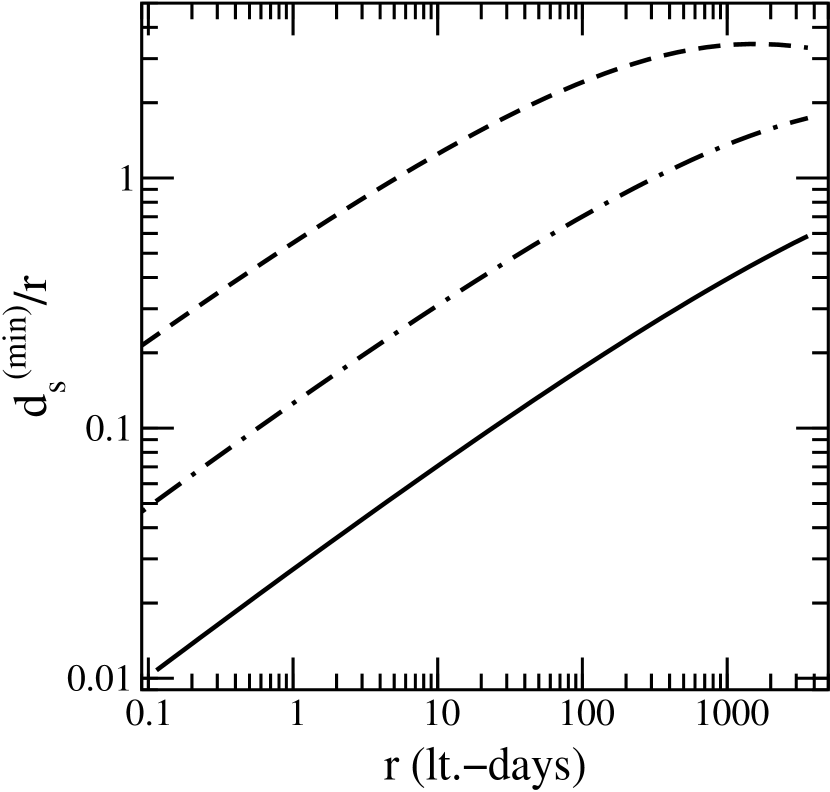
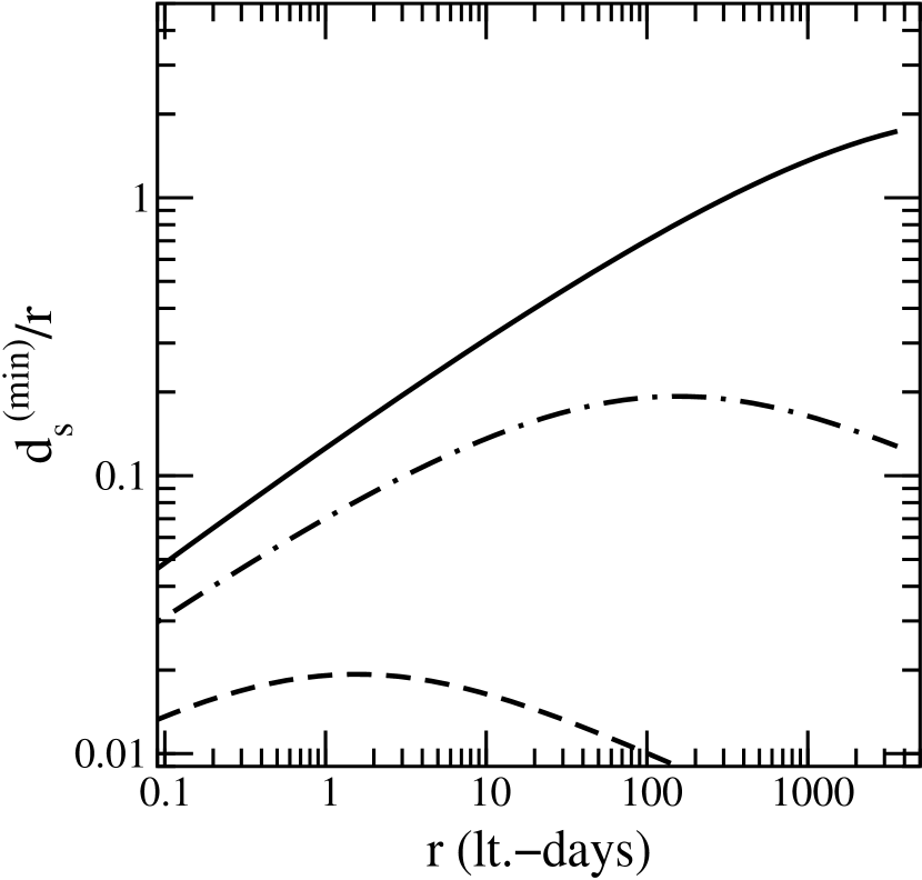
Figure 1: The minimum shock length scale required to allow clumping due to radiative cooling. Left panel: $\epsilon=0.1$; $T_{7}=1$; and $M_{8}=0.1$ (dashed), 1.0 (dot-dashed), 10.0 (solid). Right panel: $M_{8}=1$; $T_{7}=1$; and $\epsilon=0.001$ (dashed), 0.01 (dot-dashed), 0.1 (solid).

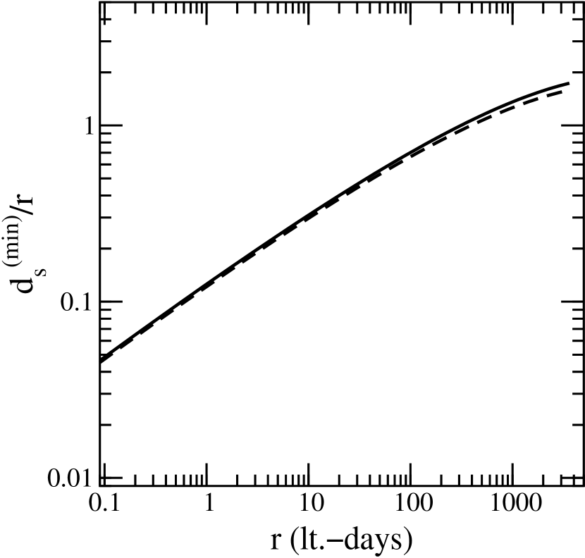
Figure 2: The minimum shock length scale required to allow clumping due to radiative cooling, with a dependence on $T_{C}$. $M_{8}=1$; $\epsilon=0.1$; and $T_{7}=0.1$ (dashed) and 1 (solid).

References

- Alexander & Netzer (1994) Alexander, T. & Netzer, H. 1994, MNRAS, 270, 781
- Alexander & Netzer (1997) Alexander, T. & Netzer, H. 1997, MNRAS, 284, 967
- Allen, Hyland & Hillier (1990) Allen, D., Hyland, A., & Hillier, D. 1990, MNRAS, 244, 706
- Arav et al. (1998) Arav, N., Barlow, T. A., Laor, A., Sargent, W. L. W., & Blandford, R. D. 1998, MNRAS, 297, 990
- Baldwin (1997) Baldwin, J. 1997, in Emission Lines in Active Galaxies: New Methods and Techniques, ed. B. M. Peterson, et al. (San Francisco: Astronomical Society of the Pacific), 80
- Bechtold et al. (1987) Bechtold, J., Weymann, R. J., Lin, Z., Malkan, M. A., 1987, ApJ, 315, 180
- Bondi & Hoyle (1944) Bondi, H, & Hoyle, F. 1944, MNRAS, 104, 273
- Bottorff et al. (1997) Bottorff, M., Korista, K. T., Shlosman, I., & Blandford, R. D. 1997, ApJ, 479, 200
- Brotherton (1996) Brotherton, M. S. 1996, ApJS, 102, 1
- Cassidy & Raine (1996) Cassidy, I., & Raine, D. J. 1996, A&A, 310, 49
- Clavel et al. (1991) Clavel, J., et al. 1991, ApJ, 366, 64
- Coker & Melia (1997) Coker, R. F., & Melia, F. 1997, ApJ, 488, L149
- Collier et al. (1998) Collier, S. J., et al. 1998, ApJ, 500, 162
- Dalgarno & Layzer (1987) Dalgarno, A., & Layzer, D. 1987, Spectroscopy of Astrophysical Plasmas (Cambridge: Cambridge University Press)
- Dietrich et al. (1998) Dietrich, M., et al. 1998, ApJS, 115, 185
- Emmering, Blandford, & Shlosman (1992) Emmering, R. T., Blandford, R. D., & Shlosman, I. 1992, ApJ, 385, 460
- Fabian et al. (1986) Fabian, A. C., Guilbert, P. W., Arnaud, K. A., Shafer, R. A., Tennant, A. F., & Ward, M. J. 1986, MNRAS, 218, 457
- Ferland et al. (1992) Ferland, G. J., Peterson, B. M., Horne, K., Welsh, W. F., & Nahar, S. N. 1992, ApJ, 387, 95
- Ferland (1996) Ferland, G. J. 1996, “Hazy, a Brief Introduction to CLOUDY”, University of Kentucky Department of Physics and Astronomy Internal Report
- Geballe, et al. (1991) Geballe, T., Krisciunas, K., Bailey, J., & Wade, R. 1991, ApJ Letters, 370, L73
- Genzel, et al. (1996) Genzel, R., Thatte, N., Krabbe, A., Kroker, H., & Tacconi-Garman, L. E. 1996, ApJ, 472, 153
- Genzel, et al. (1997) Genzel, R., Eckart, A., Ott, T. & Eisenhauer, F. 1997, MNRAS, 291, 219
- Ghez, et al. (1998) Ghez, A. M., Klein, B. L., Morris, M., & Becklin, E. E. 1998, ApJ, 509, 678
- Glenn, Schmidt, & Foltz (1994) Glenn, J., Schmidt, G. D., & Foltz, C. B. 1994, ApJ, 434, L47
- Green (1996) Green, P. J. 1996, ApJ, 467, 61
- Guilbert (1986) Guilbert, P. W. 1986, MNRAS, 218, 171
- Hall, Kleinmann & Scoville (1982) Hall, D., Kleinmann, S., & Scoville, N. 1982, ApJ Letters, 260, L53
- Jackson, et al. (1993) Jackson, J. M., Geis, N., Genzel, R., Harris, A. I., Madden, S., Poglitsch, A., Stacey, G. J., & Townes, C. H. 1993, ApJ, 402, 173
- Kaspi & Netzer (1999) Kaspi, S., & Netzer, H. 1999, ApJ, 524, 71
- Korista et al. (1995) Korista, K. T., et al. 1995, ApJS, 97, 285
- Krolik, McKee, & Tarter (1981) Krolik, J. H., McKee, C. F. & Tarter, C. B. 1981, ApJ, 249, 422
- Krabbe, et al. (1991) Krabbe, A., Genzel, R., Drapatz, S., & Rotaciuc, V. 1991, ApJ Letters, 382, L19
- Marziani, et al. (1996) Marziani, P., Sulentic, J. W., Dultzin-Hacyan, D., Calvani, M., & Moles, M. 1996, ApJS, 104, 37
- Mathews & Ferland (1987) Matthews, W. G., & Ferland, G. J. 1987, ApJ, 323, 456
- Mezger, Duschl, & Zylka (1996) Mezger, P. G., Duschl, W. J., & Zylka, R. 1996, AARv, 7, 289
- Melia (1994) Melia, F. 1994, ApJ, 426, 577
- Melia (1998) Melia, F. 1998, in the Proceedings of the 1998 Workshop on the Galactic Center, Tucson, AZ, eds. H. Falcke, F. Melia, A. Cotera, W. Duschl (Berlin: Springer Verlag), in press
- Morrison & McCammon (1983) Morrison, R. & McCammon, D. 1983, ApJ, 270, 119
- Murray & Chiang (1995) Murray, N., & Chiang, J. 1995, ApJ, 454, L105
- Murray et al. (1995) Murray, N., Chiang, J., Grossman, S. A., & Voit, G. M. 1995, ApJ, 451, 498
- Netzer (1990) Netzer, H. 1990, in Active Galactic Nuclei, ed. T. J.-L. Courvoisier & M. Mayor (Berlin: Springer-Verlag)
- O’Brien et al. (1998) O’Brien, P. T., et al. 1998, ApJ, 509, 163
- Osterbrock (1989) Osterbrock, D. E. 1989, Astrophysics of Gaseous Nebulae and Active Galactic Nuclei (Mill Valley, CA: University Science Books)
- Perry & Dyson (1985) Perry, J. J. & Dyson, J. E. 1985, MNRAS, 213, 665
- Peterson (1997) Peterson, B. M. 1997, An Introduction to Active Galactic Nuclei (Cambridge: Cambridge University Press)
- Peterson et al. (1999) Peterson, B. M., et al. 1999, ApJ, 510, 659
- Reichert et al. (1994) Reichert, G. M., et al. 1994, ApJ, 425, 582
- Reynolds & Fabian (1995) Reynolds, C. S., & Fabian, A. C. 1995, MNRAS, 273, 1167
- Robinson (1995) Robinson, A. 1995, MNRAS, 276, 933
- Rodríguez-Pascual et al. (1997) Rodríguez-Pascual, P. M., et al. 1997, ApJS, 110, 9
- Ruffert & Melia (1994) Ruffert, M., & Melia, F. 1994, A&A, 288, L29
- Santos-Lleó et al. (1997) Santos-Lleó, M., et al. 1997, ApJS, 112, 271
- Shields, Ferland & Peterson (1995) Shields, J. C., Ferland, G. J., & Peterson, B. M. 1995, ApJ, 441, 507
- Stirpe et al. (1994) Stirpe, G. M., et al. 1994, ApJ, 425, 609
- Wandel (1997) Wandel, A. 1997, ApJ, 490, L131
- Wandel, Peterson, & Malkan (1999) Wandel, A., Peterson, B. M., & Malkan, M. A. 1999, ApJ, 526, 579
- Wanders et al. (1997) Wanders, I., et al. 1997, ApJS, 113, 69
- Yusef-Zadeh & Melia, (1992) Yusef-Zadeh, F. & Melia, F. 1992, ApJ, 385, L41