Cerenkov Line-like Radiation, The Extended and Improved Formulae System

Abstract

You & Cheng (1980) argued that, for relativistic electrons moving through a dense gas, the Cerenkov effect will produce peculiar atomic and/or molecular emission lines–Cerenkov lines. They presented a series of formulae to describe the new line-mechanism. Elegant experimental confirmation has been obtained by Xu. et al. in the laboratory which definitely verified the existence of Cerenkov lines. Owing to the potential importance in high energy astrophysics, in this paper we give a more detailed physical discussion of the emission mechanisms and improve the previous formulae system into a form which is more convenient for astrophysical application. Specifically, the extended formulae in this paper can be applied to other species of atoms and/or ions rather than hydrogen as in the previous paper , and also to X-ray astronomy. They can also be used for the calculation of a nonuniform plane-parallel slab of the emissive gas.

ccretion, accretion disks – Line: profiles – X-rays: general

1 Introduction

Early in the 1980’s, You & Cheng (1980) mentioned that, when relativistic electrons pass through a dense gas region, the radiation produced by the Cerenkov effect will be concentrated into a narrow waveband $\Delta\lambda$, very near to the intrinsic atomic or molecular wavelength position $\lambda_{lu}$ ($u,l$ denote the corresponding upper and lower levels respectively). Therefore it looks more like an atomic emission line (for gas composed of atoms) and/or molecular line (for molecular gas), rather than a continuum. They called it the “Cerenkov Emission Line”. Later, they presented a series of formulae to describe the properties of the peculiar Cerenkov line (You,Kiang and Chengs, 1984, 1986). Elegant experimental confirmation of Cerenkov line in $O_{2}$, $Br_{2}$ gas, and $Na$ vapor using a ${}^{90}Sr$ $\beta$-ray source has been obtained in the laboratory (Xu et al. 1981, 1988, 1989). By use of the fast coincidence technique, they found the line emission at the expected directions, wavelengths and plane of polarization. It has been emphasized (You et al. 1986) that the Cerenkov emission line is not a real line in the precise meaning due to the following features: (I) it is rather broad, for a dense gas with $N_{H}\simeq 10^{15}{\rm cm^{-3}}$, $T\simeq 10^{4}{\rm K}$, the calculated linewidth of Cerenkov $L_{y\alpha}$ is $\Delta\lambda\simeq 1-10\AA$; (II) generally, the line profile is asymmetric, being steep on the blue side and flat on the red side; (III) its peak is not precisely at $\lambda_{lu}$, but slightly red-shifted, we call this the “Cerenkov line redshift”, so as to distinguish it from other types of redshift mechanisms (Doppler, gravitational, Compton etc.); (IV) it is polarized if the relativistic electrons have an anisotropic velocity distribution.

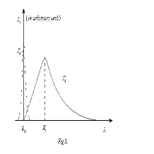
Figure 1: Comparison of the schematic profiles of the Cerenkov line $I^{c}_{\lambda}\sim\lambda$ and the normal line by spontaneous transition process $I^{s}_{\lambda}\sim\lambda$. The former has been red-shifted and has asymmetry and large linewidth.

The schematic profile of the Cerenkov line $I^{c}_{\lambda}\sim\lambda$ is shown in Fig.1, where the profile of the normal emission line $I^{s}_{\lambda}\sim\lambda$ produced by a spontaneous transition process (recombination-cascade and/or collisional excitation) is also presented for comparison.

Here, we emphasize the special importance of point (III). It is the Cerenkov line-redshift which strengthens the emergent intensity of the Cerenkov emission line. The reason is easy to understand. For an optically thick dense gas, the emergent line flux is determined both by the emission and the absorption.The absorption mechanisms for the normal lines (recombination-cascade and collisional excitation) and for the Cerenkov lines are extremely different. The line-intensity $I^{s}$ of a normal line is greatly weakened by the large resonance absorption $k_{lu}(\lambda_{lu})$ due to the fact that the normal line is located at the position of the intrinsic wavelength $\lambda=\lambda_{lu}$ (see Fig.1). where $k_{lu}(\lambda_{lu})$ is very large, $k_{lu}(\lambda_{lu})\rightarrow\infty$ (In the extreme case of a very dense gas, the emergent flux has a continuum with black body spectrum, and the line intensity $I^{s}\simeq 0$). However, the Cerenkov line, located at $\lambda>\lambda_{lu}$ because of the small “Cerenkov line-redshift” (generally, $\Delta Z^{c}\equiv\frac{\Delta\lambda_{p}}{\lambda_{lu}}\simeq 10^{-3}$, or the apparent “velocity” V a few hundred km/sec) can avoid the strong line absorption $k_{lu}$ because $k_{lu}(\lambda>\lambda_{lu})\rightarrow 0$. Therefore, the Cerenkov line intensity $I^{c}$ is only affected by a very small photoelectric absorption $k_{bf}$, and $k_{bf}\ll k_{lu}(\lambda_{lu})$, which means that the photons of the Cerenkov line can easily escape from deep inside a dense gas cloud. The depth scale is $L\simeq 1/k_{bf}\gg 1/k_{lu}(\lambda_{lu})$, causing a strong emergent intensity $I^{c}$ only if the density of fast electrons $N_{e}$ is large enough. In other words, the dense gas appears to be more “transparent” for the Cerenkov lines than for the normal lines, which makes it possible for the Cerenkov line mechanism to dominate over the normal line emission in some physical situations.

Such a new line emission mechanism has a potential importance for high energy astrophysics, particularly in X-ray astronomy. Solar flares, QSOs and other AGNs etc. would be the first candidates. It is known that there definitely exist abundant relativistic electrons and dense gas regions in these objects, which provide the right conditions for producing the Cerenkov line-like radiation. You et al. tried to explain a series of particular observation characteristics of the broad lines of QSOs and Seyfert1 galaxies by use of the new mechanism. Moderate successes have been obtained, at least qualitatively, e.g. (1) the anomalous line-intensity ratios (the steep Balmer decrement, the small ratio $L_{y\alpha}/H_{\beta}$, etc.)(You & Cheng 1987); (2) the small redshift and red-asymmetry of the broad $H_{\beta}$ line with respect to CIV $\lambda 1549$ (Cheng et al. 1990); (3) the different lag times $\tau$ of the high-ionized lines, e.g. CIV and the low-ionized lines, e.g. MgII $\lambda 2798$, $H_{\beta}$, with respect to the flare of the continuum from the central source. The progress in the study of QSOs and AGNs in recent years, both in theories and observations mean that we can now make qualitative statements on the contribution of the Cerenkov line mechanism to the broad lines of AGNs. The latest observations which seem favorable to that Cerenkov line mechanism were provided by ASCA observations of Seyfert1 galaxies, which show an iron $K_{\alpha}$ broad line with a markedly asymmetric profiles (Tanaka, et al. 1995, K. Nandra, et al. 1997, Turner, et al. 1997). The very steep blue side and strong red wing of broad $K_{\alpha}$ line might be indicative of Cerenkov line which encourages us to reexamine and improve the formulae system of the Cerenkov line mechanism given in our previous papers (You et al. 1984, 1986), in a form which is convenient for astrophysical applications. In particular, we hope that the extended formulae can be applied to other species of multi-electron complex atoms and/or ions rather than hydrogen or hydrogenic atoms as in the previous paper, which are important for the study of the broad lines of AGNs, particularly in the X-ray band. Another extension concerns the discussion on the Cerenkov line redshift in Sect. 2, where we give a generalized formula of the Cerenkov line redshift and its simplified forms in the limiting cases of high and low gas-densities respectively. We find that the conclusion of asymmetry of the line-profile is correct only for a dense gas whose density is larger than a given critical value $N^{cr.}$. When $N\ll N^{cr.}$, the profile becomes more symmetric. Finally, our new formulae system is extended to the case of a non-uniform plane-parallel slab of emission gas ($N=N(s),T=T(s)$ etc., where $s$ is the inner distance to the surface of the slab), which is also important in practice.

2 Basic Formulae

The CGSE system of units will be used throughout. This means, in particular, that all wavelengths in the following formulae will be in centimeters rather than $\AA$. The photon energy will be in ergs rather than KeV.

2.1 The refractive index $n_{\lambda}$ and the extinction coefficient $\kappa_{\lambda}$

2.1.1 Formulae for hydrogen or hydrogen-like gas

The essential point of the calculation of the spectrum of Cerenkov radiation is the evaluation of the refractive index $n$ of the gaseous medium. This is easy to understand qualitatively from the necessary condition for producing Cerenkov radiation, $V>c/n_{\lambda}$. At a given wavelength $\lambda$, the larger the index $n$, the easier the condition $V>c/n_{\lambda}$ to be satisfied, and the stronger the Cerenkov radiation at $\lambda$ will be. Therefore, in order to get the theoretical spectrum of the Cerenkov radiation, it is necessary to calculate the refractive index $n_{\lambda}$ and its dependence on $\lambda$, i.e. the dispersion curve $n_{\lambda}\sim\lambda$. For a gaseous medium, the calculation of the $n_{\lambda}\sim\lambda$ curve is easy to do. Because our main interest is in the calculation of $n_{\lambda}$ in the vicinity of $\lambda_{lu}$, we must use the rigorous formula:

$$\frac{\tilde{n}^{2}-1}{\tilde{n}^{2}+2}=\frac{4\pi}{3}N\alpha,$$ (1)

where

$$\tilde{n}=n-i\kappa$$ (2)

$\tilde{n}$ is the complex refractive index, the real part $n$ is the refractive index of the gas, the imaginary part $\kappa$ is the extinction coefficient. $N$ is the number density of the atoms, and $\alpha$ is the polarizability per atom. When the atoms are distributed over various energy levels with density $N_{a}$ in level $a$, $N\alpha$ will be replaced by $\sum_{a}N_{a}\alpha_{a}$. According to quantum theory, the atomic polarizability per atom in level $a$ is given as (e.g. Handbook of Physics ed. Condon and Odishaw, 1958):

$$\alpha_{a}(\omega)=\frac{e^{2}}{m}\sum\limits_{a\not=b}\frac{f_{ab}}{(\omega^{2}_{ab}-\omega^{2})+i\Gamma_{ab}\omega}$$ (3)

where $e$ and $m$ are the charge and the mass of an electron, $f_{ab}$ and $\Gamma_{ab}$ are the oscillation strength and the damping constant for the atomic line of frequency $\omega_{ab}$. Substituting Eq.(3) into Eq.(1), we get:

$$N\alpha=\sum\limits_{a}N_{a}\alpha_{a}=\sum\limits_{a}N_{a}\sum\limits_{b\not=a}\frac{e^{2}}{2\pi m}\frac{f_{ab}}{2\pi(\nu^{2}_{ab}-\nu^{2})+i\Gamma_{ab}\nu}$$ (4)

Because we are concerned with the neighborhood of a given atomic line $\lambda_{lu}$, or the intrinsic frequency $\nu_{lu}$, $\nu\simeq\nu_{lu}$ ( the subscripts $u$ and $l$ denote the upper and lower-levels corresponding to the intrinsic frequency $\nu_{lu}$), it follows that we only need to keep the two largest terms in the above summation, Eq.(4) becomes:

$$N\alpha\simeq N_{l}\alpha_{lu}+N_{u}\alpha_{ul}$$ (5)

where

$$\alpha_{lu}=\frac{e^{2}}{2\pi m}\frac{f_{lu}}{2\pi(\nu^{2}_{lu}-\nu^{2})+i\Gamma_{lu}\nu}$$ (6)

and $\alpha_{ul}$ is obtained from Eq.(6) by replacing $f_{lu}$ by $f_{ul}$. Note that $f_{lu}$ and $f_{ul}$ represent the absorption and emission oscillation strengths respectively, corresponding to the pair of energy levels $(l,u)$ of a given atom. Therefore, $f_{lu}$ and $f_{ul}$ are related to each other through the statistical weights $g_{l}$ and $g_{u}$, $g_{l}f_{lu}=-g_{u}f_{ul}$. The absorption oscillation strength $f_{lu}$ is related with Einstein’s spontaneous emission coefficient $A_{ul}$ as (Bethe & Salpeter 1957):

$$f_{lu}=\frac{mc^{3}}{8\pi^{2}e^{2}\nu^{2}_{lu}}\left(\frac{g_{u}}{g_{l}}\right)A_{ul}$$ (7)

and the damping constant $\Gamma_{lu}$ is also related with Einstein’s coefficient $A_{ul}$ as:

$$\Gamma_{lu}=\Gamma_{l}+\Gamma_{u}=\sum\limits_{i(<l)}A_{li}+\sum\limits_{j(<u)}A_{uj}$$ (8)

Using these relations, Eq. (1) becomes:

$$\frac{\tilde{n}^{2}-1}{\tilde{n}^{2}+2}=\frac{b}{z+ig}$$ (9)

with

$$b\equiv\frac{c^{3}}{12\pi^{2}}\nu^{-2}_{lu}A_{ul}g_{u}\left(\frac{N_{l}}{g_{l}}-\frac{N_{u}}{g_{u}}\right)$$

$$z\equiv 2\pi\left(\nu^{2}_{lu}-\nu^{2}\right)$$ (10)

$$g\equiv\Gamma_{lu}\nu$$

From Eq. (9) and Eq. (2), we obtain the refractive index $n_{\nu}$ and the extinction coefficient $\kappa_{\nu}$ as:

$$n^{2}_{\nu}=\left[\left(A^{2}+9b^{2}g^{2}\right)^{1/2}+A\right]/2B$$

$$\kappa^{2}_{\nu}=\left[\left(A^{2}+9b^{2}g^{2}\right)^{1/2}-A\right]/2B$$ (11)

where

$$A\equiv(z+2b)(z-b)+g^{2}$$

$$B\equiv(z-b)^{2}+g^{2}$$

Eq. (11) is the $n^{2}_{\nu}\sim\nu$ dispersion formula, which we need. The $n^{2}_{\nu}\sim\nu$ dispersion curve can be easily obtained by the digital calculation by use of Eq. (11).

However, as a good approximation, Eq. (11) can be replaced by a simple analytic formula as follows. For convenience in comparing with the observations, it is better to replace the frequency $\nu$ in Eq. (9) by wavelength $\lambda$, let $\Delta\lambda\equiv\lambda-\lambda_{lu}$ represent the wavelength displacement, and let

$$y\equiv\frac{\lambda-\lambda_{lu}}{\lambda_{lu}}=\frac{\Delta\lambda}{\lambda_{lu}}$$ (12)

denote the fractional displacement, $y\ll 1$ because we are always interested in the calculation in the neighborhood of $\lambda_{lu}$, $\lambda\simeq\lambda_{lu}$. Therefore the small dimensionless quantity $y$ will be very useful in theoretical analysis (e.g. the expansion series by use of the small quantity $y$). Replacing $\nu\rightarrow\lambda$ in Eq. (11), $\nu=c/\lambda=c\lambda^{-1}_{lu}(1+y)^{-1}$, and $\nu_{lu}=c\lambda^{-1}_{lu}$. Substituting this into Eq. (10) and Eq. (11), and keeping only the terms of the lowest order in $y$, we get:

$$b=\frac{c}{12\pi^{2}}\lambda^{2}_{lu}A_{ul}g_{u}\left(\frac{N_{l}}{g_{l}}-\frac{N_{u}}{g_{u}}\right)$$

$$z=4\pi c^{2}\lambda^{-2}_{lu}y$$ (13)

$$g=c\lambda^{-1}_{lu}\Gamma_{lu}$$

Therefore, among the three quantities $b$, $g$ and $z$, only $z$ is $\Delta\lambda$-dependent. Because the Cerenkov line emission is not located in the exact position $\lambda=\lambda_{lu}$, it has a small redshift, so $y$ is not an indefinitely small quantity ($y\not\rightarrow 0$, in fact, at $y=0$, i.e. $\lambda=\lambda_{lu}$, the Cerenkov radiation disappears). In the actually effective range of $y$, we always have:

$$g\ll z,\leavevmode\nobreak\ \leavevmode\nobreak\ \leavevmode\nobreak\ \leavevmode\nobreak\ b\ll z$$ (14)

For example, for $Ly\alpha$, $l=1,u=2,\lambda_{12}=1.216\times 10^{-5}{\rm cm},\Gamma_{12}=A_{21}=6.25\times 10^{8}{\rm sec^{-1}}$. Inserting these value in Eq. (13), we find that $g\ll z$ whenever $\Delta\lambda\geq 2.0\times 10^{-4}\AA$ (equivalently, $y\geq 10^{-7}$). On the other hand, under ordinary physical conditions, we can safely assume $N_{2}\ll N_{1}\sim N$. Then even for $N_{1}$ as high as $N_{1}\simeq N\simeq 10^{17}{\rm cm^{-3}}$, $b\ll z$ will be true whenever $\Delta\lambda$ is greater than $1.1\times 10^{-3}\AA$ (or $y\geq 10^{-6}$). A smaller $N$ will give a still lower limit of $\Delta\lambda$. Therefore, the inequalities (14) always hold in the actually effective Cerenkov line-width ($\Delta\lambda\simeq 1-10\AA$). For the other lines, we obtain the same conclusion (14), under similar considerations. Thus we need only retain the terms of the lowest order of the small quantities $g/z$ and $b/z$ in Eq. (11), and we obtain:

$$n^{2}-1\simeq 3\frac{b}{z}$$

$$\kappa\simeq\frac{2}{3}\left(\frac{b}{z}\right)\left(\frac{g}{z}\right)$$ (15)

Substituting Eq. (13) into Eq. (15), finally we have the simplified approximate formulae:

$$n^{2}-1=\frac{1}{16\pi^{3}c}\lambda^{4}_{lu}A_{ul}g_{u}\left(\frac{N_{l}}{g_{l}}-\frac{N_{u}}{g_{u}}\right)y^{-1}$$

$$\kappa=\frac{1}{128\pi^{4}c^{2}}\lambda^{5}_{lu}\Gamma_{lu}A_{ul}g_{u}\left(\frac{N_{l}}{g_{l}}-\frac{N_{u}}{g_{u}}\right)y^{-2}$$ (16)

Eqs.(16) are the approximate analytic formulae for $n$ and $\kappa$ respectively. From Eq. (16) we see that $n_{\lambda}$ varies as $(n^{2}-1)\propto y^{-1}\propto\Delta\lambda^{-1}$. We shall see below that the Cerenkov spectral emissivity varies approximately as $J_{\lambda}\propto n^{2}-1$, so $J_{\lambda}\propto\Delta\lambda^{-1}$. However, the absorption varies as $\kappa_{\lambda}\propto y^{-2}\propto\Delta\lambda^{-2}$, i.e. the absorption decreases with $\Delta\lambda$ more rapidly than the emissivity. That is why we have a net Cerenkov radiation at the position $\lambda=\lambda_{lu}+\Delta\lambda$, if $\Delta\lambda$ is not approaching to zero.

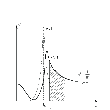
Figure 2: Relation between refractive index $n$ and wavelength $\lambda$, and relation between extinction coefficient and wavelength. The Cerenkov radiation survives in the shaded narrow region.

The calculated $n_{\lambda}\sim\lambda$ and $\kappa_{\lambda}\sim\lambda$ curves are shown in Fig. 2. The shaded region (in Fig. 2) represents a narrow waveband $\Delta\lambda$, very near to the position of intrinsic wavelength $\lambda_{lu}$, but with small redshift, where the extinction $\kappa_{\lambda}\simeq 0$, and the net Cerenkov radiation survives. The waveband $\Delta\lambda$ is so narrow(e.g. a few $\AA$), that looks more like a line-emission, rather than a continuum.

2.1.2 Extended formulae for gas of complex atoms(ions) in optical waveband

We emphasize that our derivation from Eq. (4) to Eq. (16) is limited to gas composed of hydrogen and/or hydrogen-like atoms(ions), e.g. $Na,He^{+},Fe^{+25}$, etc. However, a necessary extention to other multi-electron atoms (ions) can easily be done when we notice that Eq. (3) represents the contribution of an electron lying in the atomic energy level $a$ to the atomic polarizability $\alpha$. Therefore, for a given emission line of a given multi-electron atom with frequency $\nu_{lu}$, the quantity $N\alpha$ in Eq. (1) and (5) has to be replaced by $N(S_{l}\alpha_{lu}+S_{u}\alpha_{ul})$, i.e.

$$N\alpha\simeq N_{l}\alpha_{lu}+N_{u}\alpha_{ul}\Longrightarrow N(S_{l}\alpha_{lu}+S_{u}\alpha_{ul})\leavevmode\nobreak\ \leavevmode\nobreak\ \leavevmode\nobreak\ \leavevmode\nobreak\ \leavevmode\nobreak\ \leavevmode\nobreak\ \leavevmode\nobreak\ \leavevmode\nobreak\ \leavevmode\nobreak\ \leavevmode\nobreak\ \leavevmode\nobreak\ (5^{\prime})$$

where $N$ is the number density of complex atoms. $S_{l}$ (or $S_{u}$) represents the actual occupation number of the electrons at the lower level $l$ (or upper level $u$) of complex atom. Obviously we have

$$S_{l}\leq g_{l}\leavevmode\nobreak\ \leavevmode\nobreak\ \leavevmode\nobreak\ \leavevmode\nobreak\ {\rm and}\leavevmode\nobreak\ \leavevmode\nobreak\ \leavevmode\nobreak\ \leavevmode\nobreak\ \leavevmode\nobreak\ S_{u}\leq g_{u}$$

where $g_{l}$ and $g_{u}$ are the degeneracy of level $l$ and $u$ respectively. From Eq. (1), ($5^{\prime}$) and equality $g_{l}f_{lu}=-g_{u}f_{ul}$, it is easy to see that, if the levels ($l$, $u$) have been fully occupied by electrons (‘closed shell’), i.e. $S_{l}=g_{l}$ and $S_{u}=g_{u}$, then we have $N\alpha=0$, thus $\tilde{n}_{\nu}=n_{\nu}-i\kappa_{\nu}=1$. In other words, for the multi-electron complex atoms, the Cerenkov line-like emission related to frequency $\nu_{lu}$ can occur only when the upper and/or lower levels ($l,u$) are not fully occupied, i.e. $S_{l}<g_{l}$, and/or $S_{u}<g_{u}$ . In this case, the formulae for quantities $Z$ and $g$ in Eq. (9) are same as in Eq. (10), but the representation of quantity $b$ has to be changed. When $N_{l}\alpha_{lu}+N_{u}\alpha_{ul}$ is replaced by $N(S_{l}\alpha_{lu}+S_{u}\alpha_{ul})$, we obtain

$$b\equiv\frac{c^{3}}{12\pi^{2}}\nu^{-2}_{lu}A_{ul}g_{u}N\left(\frac{S_{l}}{g_{l}}-\frac{S_{u}}{g_{u}}\right)\leavevmode\nobreak\ \leavevmode\nobreak\ \leavevmode\nobreak\ \leavevmode\nobreak\ \leavevmode\nobreak\ \leavevmode\nobreak\ \leavevmode\nobreak\ \leavevmode\nobreak\ \leavevmode\nobreak\ \leavevmode\nobreak\ \leavevmode\nobreak\ \leavevmode\nobreak\ \leavevmode\nobreak\ \leavevmode\nobreak\ \leavevmode\nobreak\ \leavevmode\nobreak\ \leavevmode\nobreak\ \leavevmode\nobreak\ \leavevmode\nobreak\ \leavevmode\nobreak\ \leavevmode\nobreak\ \leavevmode\nobreak\ \leavevmode\nobreak\ \leavevmode\nobreak\ \leavevmode\nobreak\ (10^{\prime})$$

or

$$b\equiv\frac{c}{12\pi^{2}}\lambda^{2}_{lu}A_{ul}g_{u}N\left(\frac{S_{l}}{g_{l}}-\frac{S_{u}}{g_{u}}\right)\leavevmode\nobreak\ \leavevmode\nobreak\ \leavevmode\nobreak\ \leavevmode\nobreak\ \leavevmode\nobreak\ \leavevmode\nobreak\ \leavevmode\nobreak\ \leavevmode\nobreak\ \leavevmode\nobreak\ \leavevmode\nobreak\ \leavevmode\nobreak\ \leavevmode\nobreak\ \leavevmode\nobreak\ \leavevmode\nobreak\ \leavevmode\nobreak\ \leavevmode\nobreak\ \leavevmode\nobreak\ \leavevmode\nobreak\ \leavevmode\nobreak\ \leavevmode\nobreak\ \leavevmode\nobreak\ \leavevmode\nobreak\ \leavevmode\nobreak\ \leavevmode\nobreak\ \leavevmode\nobreak\ (13^{\prime})$$

Thus the final forms of the Eq. (16) for gas composed of multi-electron complex atoms (ions) become

$$n^{2}-1=\frac{1}{16\pi^{3}c}\lambda^{4}_{lu}A_{ul}g_{u}N\left(\frac{S_{l}}{g_{l}}-\frac{S_{u}}{g_{u}}\right)y^{-1}$$

$$\kappa_{\lambda}=\frac{1}{128\pi^{4}c^{2}}\lambda^{5}_{lu}\Gamma_{lu}A_{ul}g_{u}N\left(\frac{S_{l}}{g_{l}}-\frac{S_{u}}{g_{u}}\right)y^{-2}\leavevmode\nobreak\ \leavevmode\nobreak\ \leavevmode\nobreak\ \leavevmode\nobreak\ \leavevmode\nobreak\ \leavevmode\nobreak\ \leavevmode\nobreak\ \leavevmode\nobreak\ (16^{\prime})$$

In the following sections of this paper, all formulae from Eq. (17) to Eq. (42) are used for hydrogen and hydrogen-like gas both for simplicity and practicality because hydrogen is the most abundant element in the cosmological plasmas. However, most of these equations are valid for the multi-electron complex atoms only if the following replacement is made:

$$\left(\frac{N_{l}}{g_{l}}-\frac{N_{u}}{g_{u}}\right)\Longrightarrow N\left(\frac{S_{l}}{g_{l}}-\frac{S_{u}}{g_{u}}\right)\leavevmode\nobreak\ \leavevmode\nobreak\ \leavevmode\nobreak\ \leavevmode\nobreak\ \leavevmode\nobreak\ \leavevmode\nobreak\ \leavevmode\nobreak\ \leavevmode\nobreak\ \leavevmode\nobreak\ \leavevmode\nobreak\ \leavevmode\nobreak\ \leavevmode\nobreak\ \leavevmode\nobreak\ \leavevmode\nobreak\ \leavevmode\nobreak\ \leavevmode\nobreak\ \leavevmode\nobreak\ \leavevmode\nobreak\ \leavevmode\nobreak\ \leavevmode\nobreak\ \leavevmode\nobreak\ \leavevmode\nobreak\ \leavevmode\nobreak\ (5^{\prime})$$

2.1.3 Extended formulae for complex atoms(ions) gas in the X-ray waveband

Another important extension, which we would like to emphasize in this paper, is related to the possible application of Cerenkov line-like emission in X-ray astronomy because the waveband of some Cerenkov lines of complex atoms (ions), particularly the heavy elements, is in the X-ray range. A possible application of the Cerenkov line mechanism in the X-ray band may be a new explanation for the origin of the broad $K_{\alpha}\sim 6.4{\rm KeV}$ line of Fe ions observed in Seyfert AGNs in recent years. For convenience in comparing with the observations in the X-ray waveband, it is better to replace the wavelength $\lambda$ in the formulae given above by the frequency $\nu$, or equivalently, by the photon energy $\epsilon=h\nu$. This is easy to do without any remarkable changes in above formulae. We notice that the dimensionless small quantity $y$ in Eq. (12) can also be written as

$$y\equiv\frac{\lambda-\lambda_{lu}}{\lambda_{lu}}\equiv\frac{\Delta\lambda}{\lambda_{lu}}=-\frac{\Delta\nu}{\nu_{lu}}=-\frac{\Delta\epsilon}{\epsilon_{lu}}\leavevmode\nobreak\ \leavevmode\nobreak\ \leavevmode\nobreak\ \leavevmode\nobreak\ \leavevmode\nobreak\ \leavevmode\nobreak\ \leavevmode\nobreak\ \leavevmode\nobreak\ \leavevmode\nobreak\ \leavevmode\nobreak\ \leavevmode\nobreak\ \leavevmode\nobreak\ \leavevmode\nobreak\ \leavevmode\nobreak\ \leavevmode\nobreak\ \leavevmode\nobreak\ \leavevmode\nobreak\ \leavevmode\nobreak\ \leavevmode\nobreak\ \leavevmode\nobreak\ \leavevmode\nobreak\ \leavevmode\nobreak\ (12^{\prime})$$

where $\epsilon_{lu}\equiv h\nu_{lu}=\epsilon_{u}-\epsilon_{l}$ represents the energy difference of the upper and lower levels ($u,l$), and $-\Delta\epsilon=h\nu_{lu}-h\nu=\epsilon_{lu}-\epsilon$. i.e. the small quantity $y$ also represents the fractional displacement of the frequency or photon-energy. Inserting Eq. ($12^{\prime}$) into the equations given above we obtain the following formulae which are suitable to the application to X-ray astronomy:

$$n^{2}_{\nu}-1=\frac{c^{3}h^{4}}{16\pi^{3}}\epsilon^{-4}_{lu}A_{ul}g_{u}N\left(\frac{S_{l}}{g_{l}}-\frac{S_{u}}{g_{u}}\right)y^{-1}$$

$$\kappa_{\nu}=\frac{c^{3}h^{4}}{128\pi^{4}}\epsilon^{-5}_{lu}\Gamma_{lu}A_{ul}g_{u}N\left(\frac{S_{l}}{g_{l}}-\frac{S_{u}}{g_{u}}\right)y^{-2}\leavevmode\nobreak\ \leavevmode\nobreak\ \leavevmode\nobreak\ \leavevmode\nobreak\ \leavevmode\nobreak\ \leavevmode\nobreak\ \leavevmode\nobreak\ \leavevmode\nobreak\ \leavevmode\nobreak\ \leavevmode\nobreak\ \leavevmode\nobreak\ \leavevmode\nobreak\ (16^{\prime\prime})$$

2.2 The Cerenkov spectral emissivity $J^{c}_{\lambda}(J^{c}_{y})$ and the line width $\Delta\lambda^{c}_{\rm lim}(y_{\rm lim})$

2.2.1 Formulae for hydrogen or hydrogen-like gas

The Cerenkov spectral emissivity can be derived from the dispersion curve $n_{\lambda}\sim\lambda$ given above. It is known from the theory of Cerenkov radiation that the power emitted in a frequency interval ($\nu,\nu+d\nu$) by an electron moving with velocity ($\beta=V/c$) is $P_{\nu}d\nu=(4\pi^{2}e^{2}\beta\nu/c)\left(1-\frac{1}{n^{2}_{\nu}\beta^{2}}\right)d\nu$. Let $N(\gamma)d\gamma$ be the number density of fast electrons in the energy interval ($\gamma,\gamma+d\gamma$), ($\gamma=\frac{1}{\sqrt{1-\beta^{2}}}=mc^{2}/m_{0}c^{2}$ is the Lorentz factor, which represents the dimensionless energy of the electron), then the power emitted in interval ($\nu,\nu+d\nu$) by these electrons is $N(\gamma)d\gamma P_{\nu}d\nu$. For an isotropic velocity distribution of the relativistic electrons as in normal astrophysical conditions, the Cerenkov radiation will also be isotropic(the definite angular distribution of the Cerenkov emission disappears when the relativistic electrons have an isotropic distribution of velocities). Hence, the spectral emissivity per unit volume and unit solid angle is:

$$J^{c}_{\nu}d\nu=\frac{1}{4\pi}\int^{\gamma_{2}}_{\gamma_{1}}N(\gamma)d\gamma P_{\nu}d\nu$$

$$\leavevmode\nobreak\ \leavevmode\nobreak\ \leavevmode\nobreak\ \leavevmode\nobreak\ \leavevmode\nobreak\ \leavevmode\nobreak\ =\frac{\pi e^{2}}{c}\nu d\nu\int_{\gamma_{1}}^{\gamma_{2}}N(\gamma)d\gamma\beta\left(1-\frac{1}{n^{2}\beta^{2}}\right)$$ (17)

where, $\gamma_{1},\gamma_{2}$ are the lower and upper limit of the energy spectrum of the relativistic electrons respectively. For the relativistic electrons, we always have $\beta\simeq 1$, $\gamma\gg 1$, so $\beta^{-2}\simeq 1+\gamma^{-2}$, $\beta\simeq 1-\frac{1}{2}\gamma^{-2}$. Also we notice that in the actual effective emission range, the actual refractive index $n$ of a gas is not far from unity, $n\sim 1$ (see Eq. (16)). Therefore:

$$\int_{\gamma_{1}}^{\gamma_{2}}N(\gamma)\left(1-\frac{1}{n^{2}\beta^{2}}\right)\beta d\gamma\simeq\int_{\gamma_{1}}^{\gamma_{2}}\left(n^{2}-1-\gamma^{-2}\right)N(\gamma)d\gamma$$

$$\leavevmode\nobreak\ \leavevmode\nobreak\ \leavevmode\nobreak\ \leavevmode\nobreak\ \leavevmode\nobreak\ \leavevmode\nobreak\ \leavevmode\nobreak\ \leavevmode\nobreak\ \leavevmode\nobreak\ \leavevmode\nobreak\ \leavevmode\nobreak\ \leavevmode\nobreak\ \leavevmode\nobreak\ \leavevmode\nobreak\ \leavevmode\nobreak\ \simeq\left(n^{2}-1-\gamma^{-2}_{c}\right)N_{e}$$

where, $N_{e}\equiv\int_{\gamma_{1}}^{\gamma_{2}}N(\gamma)d\gamma$ is the density of the relativistic electrons, and $\gamma_{c}$ is the characteristic energy of the electrons (or the typical energy) in a given source. The definition of $\gamma_{c}$ is $\int_{\gamma_{1}}^{\gamma_{2}}\gamma^{-2}N(\gamma)d\gamma\equiv\gamma^{-2}_{c}N_{e}$, so $\gamma_{1}<\gamma_{c}<\gamma_{2}$. Hence:

$$J^{c}_{\nu}d\nu\simeq\frac{\pi e^{2}}{c}N_{e}\nu\left(n^{2}-1-\gamma^{-2}_{c}\right)d\nu$$ (18)

Replacing $\nu$ to $\lambda$ or $y$, we have $J_{\nu}^{c}d\nu=J_{\epsilon}^{c}d\epsilon=J_{\lambda}^{c}d\lambda=J^{c}_{y}dy$ and $dy=\lambda_{lu}^{-1}d\lambda=\lambda^{-1}_{lu}(-c\nu^{-2}d\nu)$. Therefore:

$$J_{y}^{c}dy=\pi ce^{2}N_{e}\lambda^{-2}_{lu}\left(n^{2}-1-\gamma^{-2}_{c}\right)dy$$ (19)

Setting $n^{2}-1-\gamma^{-2}_{c}=0$ and inserting the expression for $n$ (Eq. (16)) into Eq. (19), we get the Cerenkov line-width $\Delta\lambda^{c}_{\rm lim}$:

$$y_{\rm lim}\equiv\frac{\Delta\lambda^{c}_{\rm lim}}{\lambda_{lu}}=C_{0}\gamma^{2}_{c}$$

$$\leavevmode\nobreak\ \leavevmode\nobreak\ \leavevmode\nobreak\ \leavevmode\nobreak\ \leavevmode\nobreak\ =\frac{1}{16\pi^{3}c}\lambda^{4}_{lu}A_{ul}g_{u}\left(\frac{N_{l}}{g_{l}}-\frac{N_{u}}{g_{u}}\right)\gamma^{2}_{c}$$ (20)

where

$$C_{0}=\frac{1}{16\pi^{3}c}\lambda^{4}_{lu}A_{ul}g_{u}\left(\frac{N_{l}}{g_{l}}-\frac{N_{u}}{g_{u}}\right)$$

The Cerenkov radiation will be cut off at the wavelength displcaement $\Delta\lambda^{c}_{\rm lim}$. Inserting Eqs. (16) and (20) into Eq. (19), the spectral emissivity becomes:

$$J^{c}_{y}dy=C_{1}N_{e}\left(y^{-1}-y^{-1}_{\rm lim}\right)dy$$ (21)

where

$$C_{1}\equiv\frac{e^{2}}{16\pi^{2}}\lambda^{2}_{lu}A_{ul}g_{u}\left(\frac{N_{l}}{g_{l}}-\frac{N_{u}}{g_{u}}\right)$$

It is obvious that the emissivity $J^{c}_{\lambda}=0$, when $y=y_{\rm lim}$ (or $\Delta\lambda=\Delta\lambda^{c}_{\rm lim}$). But for small wavelength displacement $\Delta\lambda$, $y\ll y_{\rm lim}$, we have $J_{y}^{c}dy\propto y^{-1}\propto\Delta\lambda^{-1}$, i.e. $J^{c}_{y}$ decreases with $\Delta\lambda$ slowly as $J^{c}_{y}\propto\Delta\lambda^{-1}$. Therefore, in the actual effective emission range $y\ll y_{\rm lim}$, we have a good approximation of Eq. (21)

$$J^{c}_{y}dy=C_{1}N_{e}y^{-1}dy$$ (22)

We point out that there is a remarkable difference between the Cerenkov line emission and the usual spontaneous radiation transition, the later is determined by the population density in the upper level $u$, $J^{s}\propto N_{u}$. But the Cerenkov emissivity is determined by the difference in populations between the lower and upper levels $\left(\frac{N_{l}}{g_{l}}-\frac{N_{u}}{g_{u}}\right)$.

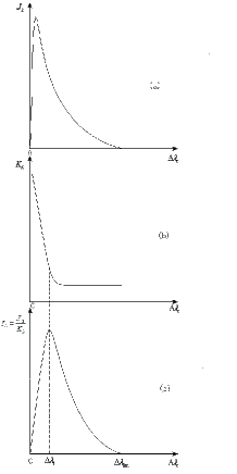
Figure 3: The Cerenkov emissivity $J_{\lambda}$ (a), absorption coefficient $k_{\lambda}$ (b), and the emergent intensity $I_{\lambda}$ of the Cerenkov line (optically thick case) (c). From (c) we see, the Cerenkov linewidth is large. The line profile is asymmetric with a small redshift.

The original profile of the Cerenkov line is given by the calculated curve $J^{c}_{y}\sim y$ $\left(orJ^{c}_{\epsilon}\sim\Delta\epsilon,orJ^{c}_{\lambda}\sim\Delta\lambda\right)$, as shown in Fig. 3(a) which is obtained from Eq. (22). However, for the small wavelength displacement $\Delta\lambda\simeq 0$, i.e. $\lambda$ is very close to $\lambda_{lu}$, the approximate Eq. (22) has to be replaced by the strict Eq. (11) and Eq. (17).

2.2.2 Extended formulae of $J^{c}_{y}$ and $y^{c}_{\rm lim}$ for complex atoms(ions) or molecules gas

The basic formulae for Cerenkov spectral emissivity $J^{c}_{y}$ and maximum line-width $y_{\rm lim}$, Eq. (20), Eq. (21) and Eq. (22) can be easily extended to the multi-electron complex atoms(ions) or molecular gas by use of the same simple replacement given by Eq. ($5^{\prime}$) in Sect. 2.1.2, i.e. $N_{l}\rightarrow NS_{l}$, $N_{u}\rightarrow NS_{u}$. This is sufficient for the Cerenkov line of complex atoms in the optical band. However, if the Cerenkov line is located in the X-ray band, e.g. the Cerenkov Fe $K_{\alpha}$ line at $\sim 6.4{\rm KeV}$, it is more convenient to replace the wavelength $\lambda$ in Eqs. (20), (21) and (22) by the photon energy $\epsilon=h\nu$, $\lambda_{lu}\rightarrow\epsilon_{lu}=\frac{hc}{\lambda_{lu}}$. This is easy to do because of the simple relation $J_{\lambda}^{c}d\lambda=J_{y}^{c}dy=J_{\epsilon}^{c}d\epsilon$ and $y=\frac{\lambda-\lambda_{lu}}{\lambda_{lu}}=\frac{\nu_{lu}-\nu}{\nu_{lu}}=\frac{\epsilon_{lu}-\epsilon}{\epsilon_{lu}}$. Therefore, the Cerenkov spectral emissivity and line-width of complex atoms in X-ray band are still given by Eq. (20), (21) and (22) respectively, but the parameters are changed as

$$C_{0}\equiv\frac{c^{3}h^{4}}{16\pi^{3}}\epsilon^{-4}_{lu}A_{ul}g_{u}N\left(\frac{S_{l}}{g_{l}}-\frac{S_{u}}{g_{u}}\right)\leavevmode\nobreak\ \leavevmode\nobreak\ \leavevmode\nobreak\ \leavevmode\nobreak\ \leavevmode\nobreak\ \leavevmode\nobreak\ \leavevmode\nobreak\ \leavevmode\nobreak\ \leavevmode\nobreak\ \leavevmode\nobreak\ \leavevmode\nobreak\ \leavevmode\nobreak\ \leavevmode\nobreak\ \leavevmode\nobreak\ \leavevmode\nobreak\ \leavevmode\nobreak\ \leavevmode\nobreak\ \leavevmode\nobreak\ (20^{\prime})$$

and

$$C_{1}\equiv\frac{e^{2}c^{2}h^{2}}{16\pi^{2}}\epsilon^{-2}_{lu}A_{ul}g_{u}N\left(\frac{S_{l}}{g_{l}}-\frac{S_{u}}{g_{u}}\right)\leavevmode\nobreak\ \leavevmode\nobreak\ \leavevmode\nobreak\ \leavevmode\nobreak\ \leavevmode\nobreak\ \leavevmode\nobreak\ \leavevmode\nobreak\ \leavevmode\nobreak\ \leavevmode\nobreak\ \leavevmode\nobreak\ \leavevmode\nobreak\ \leavevmode\nobreak\ \leavevmode\nobreak\ \leavevmode\nobreak\ \leavevmode\nobreak\ \leavevmode\nobreak\ \leavevmode\nobreak\ \leavevmode\nobreak\ (21^{\prime})$$

We emphasize again that $\epsilon_{lu}=\epsilon_{u}-\epsilon_{l}$ in Eq. ($20^{\prime}$) and ($21^{\prime}$) is in unit of ergs in CGSE system, rather than in KeV as usually used in the X-ray astronomy.

2.3 The absorption coefficient

2.3.1 Formulae for hydrogen and hydrogen-like gas

For an optically thick dense gas for which the Cerenkov line mechanism is efficient, the final emergent intensity $I^{c}_{\lambda}$ is determined by the competition between the emission $J^{c}_{\lambda}$ and the absorption $k_{\lambda}$. Therefore it is necessary to consider the absorption of the gas at $\lambda\simeq\lambda_{lu}$. For the optical and X-ray wavebands, there are two main absorption mechanisms that are relevant to the Cerenkov line emission. One is the line absorption $k_{lu}$ in the vicinities of atomic lines, directly related to the extinction coefficient $\kappa$ given in Eqs. (11) and (16) by the relation $k_{lu}=4\pi\kappa/\lambda$. Another is the photoelectric absorption $k_{bf}$, the free-free absorption $k_{ff}$ is very small in the optical or X-ray band in which we are mainly interested, and can be neglected. Thus, for us, in the dust-free case, the total absorption is:

$$k=k_{lu}+k_{bf}$$ (23)

$k_{lu}$ can be obtained from the well known formula in molecular optics, $k_{lu}=\frac{4\pi}{\lambda}\kappa_{\lambda}=\frac{4\pi}{\lambda_{lu}}(1-y)\kappa_{\lambda}\simeq\frac{4\pi}{\lambda_{lu}}\kappa_{\lambda}$. Using Eq. (16) and retaining the lowest order of $y$, we have:

$$k_{lu}=\frac{1}{32\pi^{3}c^{2}}\lambda^{4}_{lu}A_{ul}\Gamma_{lu}g_{u}\left(\frac{N_{l}}{g_{l}}-\frac{N_{u}}{g_{u}}\right)y^{-2}=C_{2}y^{-2}$$ (24)

where

$$C_{2}\equiv\frac{1}{32\pi^{3}c^{2}}\lambda^{4}_{lu}A_{ul}\Gamma_{lu}g_{u}\left(\frac{N_{l}}{g_{l}}-\frac{N_{u}}{g_{u}}\right)$$

Therefore the resonance absorption $k_{lu}\propto\Delta\lambda^{-2}$ decreases rapidly with $\Delta\lambda$.

Here, we point out that $k_{lu}$ can be obtained in another way which is more familiar to astronomers. The well known formula for line absorption is:

$$k_{lu}=\frac{c^{2}N_{l}}{8\pi\nu^{2}}\left(\frac{g_{u}}{g_{l}}\right)\left(1-\frac{g_{l}N_{u}}{g_{u}N_{l}}\right)A_{ul}\varphi_{ul}(\nu)$$

where, $\varphi_{ul}(\nu)$ is the Lorentz profile factor

$$\varphi_{ul}(\nu)=\frac{\Gamma_{lu}/4\pi^{2}}{(\nu-\nu_{lu})^{2}+(\Gamma_{lu}/4\pi)^{2}}\simeq\frac{\Gamma_{lu}}{4\pi^{2}(\nu-\nu_{lu})^{2}}$$

Combining these two expressions, we obtain Eq. (24) again.

The photoionization absorption coefficient is $k_{bf}=\sum_{s}N_{s}\sigma_{bf}(s)$, where the summation extends over all levels for which the photoionization potential is less than incident photon energy $h\nu$, $I_{s}\leq h\nu$. In normal astrophysical conditions, the most important photoionization absorber is the neutral hydrogen due to its great abundance. Therefore, in optical wavebands we only consider the absorption by neutral hydrogen in the calculation of $k_{bf}$ ($H_{e}$ is the next candidate in the detailed calculation). The photoelectric cross section of level s of the hydrogen atoms is:

$$\sigma_{bf}(s)=2.8\times 10^{29}\nu^{-3}s^{-5}$$

or

$$\sigma_{bf}(s)=1.04\times 10^{-2}s^{-5}\lambda^{3}_{lu}(1+y)^{3}\simeq 1.04\times 10^{-2}s^{-5}\lambda^{3}_{lu}$$

(we keep the lowest order of $y$) Therefore

$$k_{bf}\simeq 1.04\times 10^{-2}\lambda^{3}_{lu}\sum\limits_{s\geq p}N_{H^{0}_{s}}s^{-5}$$

$$\leavevmode\nobreak\ \leavevmode\nobreak\ \leavevmode\nobreak\ \leavevmode\nobreak\ \leavevmode\nobreak\ \simeq 1.04\times 10^{-2}\lambda^{3}_{lu}N_{H^{0}_{p}}p^{-5}$$ (25)

The last approximation step in Eq. (25) means that only the absorption of the lowest photoelectric level $s=p$ (i.e. the largest term in the summation) is taken into consideration. The calculated $k_{\lambda}=k_{lu}+k_{bf}\sim\Delta\lambda$ curve is shown in Fig. 3(b). Comparing Eq. (25) with Eq. (24), we see that the line absorption $k_{lu}\propto y^{-2}$ decreases rapidly with increasing $y$, so $k_{lu}$ is effective only in a very narrow range near to $\lambda_{lu}$, while the photoelectric absorption $k_{bf}$ is nearly independent of wavelength displacement $\Delta\lambda$ (or $y$). Over the whole width of the Cerenkov line, $k_{bf}$ is actually the main absorption that determines the integrated emergent intensity. The main effect of $k_{lu}$ is to shift the line towords the red side of $\lambda_{lu}$ (i.e. the Cerenkov line redshift).

2.3.2 Extended formulae of absorption $k$ for complex atoms(ions) gas

As for the complex atoms(ions), the absorption coefficient $k$ is still given by Eq. (23), where the line absorption $k_{lu}$ is still given by Eq. (24), $k_{lu}=C_{2}y^{-2}$. But the parameter $C_{2}$ is expressed as

$$C_{2}\equiv\frac{1}{32\pi^{3}c^{2}}\lambda^{4}_{lu}A_{ul}\Gamma_{ul}g_{u}N\left(\frac{S_{l}}{g_{l}}-\frac{S_{u}}{g_{u}}\right)\leavevmode\nobreak\ \leavevmode\nobreak\ \leavevmode\nobreak\ \leavevmode\nobreak\ \leavevmode\nobreak\ \leavevmode\nobreak\ \leavevmode\nobreak\ \leavevmode\nobreak\ \leavevmode\nobreak\ \leavevmode\nobreak\ \leavevmode\nobreak\ \leavevmode\nobreak\ \leavevmode\nobreak\ \leavevmode\nobreak\ \leavevmode\nobreak\ \leavevmode\nobreak\ (24^{\prime})$$

i.e. we use the replacement $N_{l}\rightarrow NS_{l}$, $N_{u}\rightarrow NS_{u}$, where $N$ is the density of the multi-electron complex atoms concerned. Futhermore, if the Cerenkov line is located in the X-ray band, $C_{2}$ is expressed as

$$C_{2}\equiv\frac{c^{2}h^{4}}{32\pi^{3}}\epsilon^{-4}_{lu}A_{ul}\Gamma_{ul}g_{u}N\left(\frac{S_{l}}{g_{l}}-\frac{S_{u}}{g_{u}}\right)\leavevmode\nobreak\ \leavevmode\nobreak\ \leavevmode\nobreak\ \leavevmode\nobreak\ \leavevmode\nobreak\ \leavevmode\nobreak\ \leavevmode\nobreak\ \leavevmode\nobreak\ \leavevmode\nobreak\ \leavevmode\nobreak\ \leavevmode\nobreak\ \leavevmode\nobreak\ \leavevmode\nobreak\ \leavevmode\nobreak\ \leavevmode\nobreak\ \leavevmode\nobreak\ \leavevmode\nobreak\ \leavevmode\nobreak\ \leavevmode\nobreak\ \leavevmode\nobreak\ (24^{\prime\prime})$$

where $\epsilon_{lu}$ is in ergs. i.e. we have used the replacement $\lambda_{lu}=\frac{hc}{\epsilon_{lu}}$ in Eq. ($24^{\prime}$) to get ($24^{\prime\prime}$).

However, when the Cerenkov line is in the X-ray band, we must take care for the calculation of the second kind of absorption, the photoionization $k_{bf}$, because of the fact that the hydrogen is no longer an important species responsible for the photoelectric absorption due to its very small photoelectric absorption cross section in the X-ray band ($\sigma_{bf}\propto\nu^{-3}$, see Eq. (25)), in spite of the great abundance of hydrogen in cosmological plasma.

In fact, for a given emission line in the X-ray band, the dominant contributors to the photoelectric absorption are the heavy elements with high $Z$, including the relevant multi-electron atom itself, which produces the emission line concerned (see the frequency behaviour of the photoelectric absorption cross section shown in Eq. (26) below, which shows the cross section $\sigma_{bf}$ reaches a maximum at each absorption edge of the given atom, then decreases drastically as $\propto\nu^{-3}$). For example, for Fe $K_{\alpha}$ line at $\sim 6.4{\rm KeV}$, the dominant photoionization absorbers are approximately the iron atoms or ions themselves, rather than other elements, Ca, O, S, etc., due to the highest abundance of $Fe$ among the heavy elements with high $Z$. Furthermore, the main energy levels of the electron of the complex atom which are responsible for the photoelectric absorption are the K, L, M shells of the heavy elements. For example, for Fe $K_{\alpha}$ line $\sim 6.4{\rm KeV}$, the most important contributors to the photoelctric absorption are the electrons in L shell of Fe ions. The ionization potential of the Fe K-shell is $I_{K}\sim 7.2{\rm KeV}$, higher than $6.4{\rm KeV}$. Thus the electrons in the K-shell of the iron atom or ions can not be photoionized by the incident Fe $K_{\alpha}$ photons $\sim 6.4{\rm KeV}$. Therefore, for Fe $K_{\alpha}$ line, we have

$$k_{bf}=\sum\limits_{s\geq 2}N(Fe)S_{s}\sigma_{bf}(s)\simeq N(Fe)S_{2}\sigma_{bf}(2)\leavevmode\nobreak\ \leavevmode\nobreak\ \leavevmode\nobreak\ \leavevmode\nobreak\ \leavevmode\nobreak\ \leavevmode\nobreak\ \leavevmode\nobreak\ \leavevmode\nobreak\ \leavevmode\nobreak\ \leavevmode\nobreak\ \leavevmode\nobreak\ \leavevmode\nobreak\ (25^{\prime})$$

where $N(Fe)$ is the density of Fe in the gas, $S_{2}$ is the occupation number of electrons at $s=2$ energy level, $S_{2}\leq g_{2}$, $\sigma_{bf}(2)$ is the photoelectric cross section of an electron at $s=2$ level. The last approximation in ($25^{\prime}$) means that we only keep the largest term in the summation due to the fact that $\sigma_{bf}(2)$ is the largest one around $\sim 6.4{\rm KeV}$, comparing with $\sigma_{bf}(3)$, $\sigma_{bf}(4)$ $\cdots$, i.e. $\sigma_{bf}(2)\gg\sigma_{bf}(3)\gg\sigma_{bf}(4)$. For the Fe atom and/or ions, the hydrogen-like formula for the cross section is a good approximation, particularly for the low-lying levels $s=2,3$

$$\sigma_{bf}(\nu,s)=\frac{32\pi^{2}e^{6}R_{\infty}Z^{4}}{3\sqrt{3}h^{3}\nu^{3}s^{5}}g_{fb}(\nu,T)$$ (26)

Therefore $\sigma_{bf}(2)$ in Eq. ($25^{\prime}$) is (taking $Z^{eff.}=24$ for $s=2$ level, i.e. for electron in the L-shell, the effective $Z^{eff.}=24$)

$$\sigma_{bf}(2)\simeq 2.9\times 10^{33}/\nu^{3}\simeq 2.9\times 10^{33}/\nu_{lu}^{3}\leavevmode\nobreak\ \leavevmode\nobreak\ \leavevmode\nobreak\ ({\rm cm^{2}})$$

Inserting to Eq. ($25^{\prime}$), we get

$$k_{bf}=8.4\times 10^{-46}N(Fe)S_{2}\epsilon^{-3}_{lu}\leavevmode\nobreak\ \leavevmode\nobreak\ \leavevmode\nobreak\ \leavevmode\nobreak\ \leavevmode\nobreak\ \leavevmode\nobreak\ \leavevmode\nobreak\ \leavevmode\nobreak\ \leavevmode\nobreak\ \leavevmode\nobreak\ \leavevmode\nobreak\ \leavevmode\nobreak\ \leavevmode\nobreak\ \leavevmode\nobreak\ \leavevmode\nobreak\ \leavevmode\nobreak\ \leavevmode\nobreak\ \leavevmode\nobreak\ \leavevmode\nobreak\ \leavevmode\nobreak\ \leavevmode\nobreak\ \leavevmode\nobreak\ \leavevmode\nobreak\ \leavevmode\nobreak\ (25^{\prime\prime})$$

where $\epsilon_{lu}\equiv\epsilon_{21}=6.4{\rm KeV}=1.025\times 10^{-8}({\rm ergs})$ in unit ergs.

2.4 The emergent spectral intensity $I^{c}_{\lambda}$ (or $I^{c}_{y}$). The line profile

In this section, we present formulae describing the Cerenkov intensity and the line profile, emergent from a plane-parallel emission slab. Similarly, we first discuss the hydrogen or hydrogen-like gas. Using the $J^{c}_{y}$ and $k_{y}$ given above, the emergent Cerenkov line intensity $I^{c}_{\lambda}$ from the surface of the slab can be calculated by the equation of radiative transfer:

$$\frac{d}{d\tau_{\lambda}}\left[\frac{I^{c}_{\lambda}(x)}{n^{2}_{\lambda}}\right]=S_{\lambda}-\frac{I^{c}_{\lambda}(x)}{n^{2}_{\lambda}}$$ (27)

where, $d\tau_{\lambda}=k_{\lambda}ds$ is the elementary optical depth, $S_{\lambda}\equiv J^{c}_{\lambda}/k_{\lambda}n^{2}_{\lambda}$ is the source function.

2.4.1 $I^{c}_{\lambda}$ (or $I^{c}_{y}$) and the line profile of the Cerenkov line of hydrogen or hydrogen-like gas

Case A. The uniform plane-parallel slab.

For a uniform plane-parallel slab of an emitting gas with thickness $L$, the solution of Eq. (27) gives the emergent spectral intensity $I^{c}_{\lambda}$:

$$I^{c}_{\lambda}=n^{2}_{\lambda}S_{\lambda}(1-e^{-\tau_{\lambda}})=\frac{J^{c}_{\lambda}}{k_{\lambda}}\left(1-e^{-k_{\lambda}L}\right)$$ (28)

where $k_{\lambda}L=\tau_{\lambda}$ is the optical thickness of the uniform slab of the emission gas. Replacing $\lambda$ by $y\equiv\Delta\lambda/\lambda_{lu}$, Eq. (28) can be expressed in an equivalent form:

$$I^{c}_{y}=\frac{J^{c}_{y}}{k_{y}}\left(1-e^{-k_{y}L}\right)$$ (29)

However, we shall be particularly interested in the optically thick case, because our main interest is in the high energy astrophysical objects, such as QSOs, supernovae, solar flares, etc., and we know that these objects all have compact structures in which the gas density is high, and near the optically thick case. On the other hand, in Sec. 1, we have argued that the Cerenkov line radiation becomes important only when the gas is dense and optically thick for continuum, i.e. $k_{\lambda}L=(k_{lu}+k_{bf})L\gg 1$. In the optically thick case, Eq. (29) becomes $I^{c}_{y}=J^{c}_{y}/k_{y}$ or

$$I^{c}_{\lambda}\simeq J^{c}_{\lambda}/k_{\lambda}$$ (30)

where, $J^{c}_{\lambda}$, $k_{\lambda}=k_{lu}+k_{bf}$ have been given in Eqs. (21), (24) and (25), in which the variable is $y=\Delta\lambda/\lambda_{lu}$, rather than $\Delta\lambda$. Therefore Eq. (30) becomes:

$$I^{c}_{y}=\frac{J^{c}_{y}}{k_{lu}+k_{bf}}=\frac{N_{e}C_{1}\left(y^{-1}-y^{-1}_{\rm lim}\right)}{C_{2}y^{-2}+k_{bf}}$$ (31)

where, $C_{1},C_{2}$ and $k_{bf}$ are given in Eqs. (21), (24) and (25) respectively, and $y^{c}_{\rm lim}=C_{0}\gamma^{2}_{c}$, $C_{0}$ is given in Eq. (20).

For convenience, we re-list the constants as follows:

$$C_{0}=\frac{1}{16\pi^{3}c}\lambda_{lu}^{4}A_{ul}g_{u}\left(\frac{N_{l}}{g_{l}}-\frac{N_{u}}{g_{u}}\right)$$

$$\leavevmode\nobreak\ \leavevmode\nobreak\ \leavevmode\nobreak\ \simeq 6.72\times 10^{-14}\lambda_{lu}^{4}A_{ul}\frac{g_{u}}{g_{l}}NR_{l}$$

$$C_{1}=\frac{e^{2}}{16\pi^{2}}\lambda_{lu}^{2}A_{ul}g_{u}\left(\frac{N_{l}}{g_{l}}-\frac{N_{u}}{g_{u}}\right)$$

$$\leavevmode\nobreak\ \leavevmode\nobreak\ \leavevmode\nobreak\ \simeq 1.46\times 10^{-21}\lambda_{lu}^{2}A_{ul}\frac{g_{u}}{g_{l}}NR_{l}$$

$$C_{2}=\frac{1}{32\pi^{3}c^{2}}\lambda_{lu}^{4}A_{lu}\Gamma_{lu}g_{u}\left(\frac{N_{l}}{g_{l}}-\frac{N_{u}}{g_{u}}\right)$$

$$\leavevmode\nobreak\ \leavevmode\nobreak\ \leavevmode\nobreak\ \simeq 1.12\times 10^{-24}\lambda_{lu}^{4}A_{ul}\Gamma_{lu}\frac{g_{u}}{g_{l}}NR_{l}$$

$$k_{bf}=1.04\times 10^{-2}\lambda^{3}_{lu}N_{H_{p}^{0}}p^{-5}$$

$$\leavevmode\nobreak\ \leavevmode\nobreak\ \leavevmode\nobreak\ =1.04\times 10^{-2}\lambda_{lu}^{3}N_{H^{0}}p^{-5}R_{p}$$ (32)

(Note that the wavelength $\lambda_{lu}$ in Eqs. (32) is in centimeter rather than $\AA$)

The last step approximation in Eqs.(32) is due to the fact that, in the normal conditions of a gaseous medium, at least for the lowest levels, we have $N\simeq N_{1}\gg N_{2}\gg N_{3}\cdots$, or $N_{l}\gg N_{u}$. So $\left(\frac{N_{l}}{g_{l}}-\frac{N_{u}}{g_{u}}\right)\simeq\frac{N_{l}}{g_{l}}=\frac{1}{g_{l}}R_{l}N$, $N$ is the total density of the hydrogen or hydrogenic atom (or ion) species concerned, e.g. $N=N(Mg^{+}),N_{H^{0}},N(Na^{0})\cdots$ for the calculation of Cerenkov lines of $MgII,HI,NaI,\cdots$. $R_{l}\equiv\frac{N_{l}}{N}$ is the fractional population in the level $l$ of the concerned atom (ion) species. Similarly, $\sum\limits_{s\geq p}N_{H^{0}_{s}}s^{-5}\simeq R_{p}N_{H^{0}}p^{-5}$, where $N_{H^{0}}$ is the number density of the neutral hydrogen atom in the uniform slab, $R_{p}\equiv N_{H^{0}_{p}}/N_{H^{0}}$ is the fractional population of the neutral hydrogen in the lowest photoelectric level $p$.

Finally, for comparison with the observations, it is necessary to transform $I^{c}_{y}$ in Eq. (31) into $I^{c}_{\lambda}$. Using $I^{c}_{y}dy=I^{c}_{\lambda}d\lambda$ and $dy=\frac{1}{\lambda_{lu}}d\lambda$, we have:

$$I^{c}_{\lambda}=\frac{1}{\lambda_{lu}}I^{c}_{y}$$ (33)

If the conventional unit (${\rm ergs/cm^{2}\cdot sec\cdot str\cdot\AA}$) is adopted for $I^{c}_{\lambda}$, then Eq. (33) becomes $I^{c}_{\lambda}=\frac{10^{-8}}{\lambda_{lu}}I^{c}_{y}$. By use of Eqs. (31), (32) and (33), the calculated profile of the Cerenkov line $I^{c}_{\lambda}\sim\Delta\lambda$ in the optically thick case is shown in Fig. 3(c), which is broad (line-width $\Delta\lambda_{\rm lim}=\lambda_{lu}y_{\rm lim}=C_{0}\lambda_{lu}\gamma^{2}_{c}$); slightly red shifted; and red-asymmetric, as mentioned above. Here we emphasized that the formula of spectral intensity Eq. (31) is obtained by the use of the approximate formulae Eqs. (16), (21) and (24), which are valid only if the condition (14), e.g. $g\ll z$, $b\ll z$, is satisfied (That is, the fractional wavelength displacement $y$ can not be indefinitely small, $y\equiv\frac{\Delta\lambda}{\lambda_{lu}}\not\rightarrow 0$. Otherwise $J^{c}_{y}\propto y^{-1}\rightarrow\infty$ and $k_{lu}\propto y^{-2}\rightarrow\infty$, which are obviously unacceptable). However, the derived formula of $I^{c}_{y}$, i.e. Eq. (31) can be safely extended to $y\rightarrow 0$ without any divergence. Particularly we have $I^{c}_{y}=0$ at $y=0$. Therefore, Eq. (31) is valid in the whole waveband of the Cerenkov line $(0,y_{\rm lim})$.

Case B. The non-uniform plane-parallel slab.

For a non-uniform plane-parallel slab of emissive gas, Eq. (28), and hence Eqs. (29)–(31) are no longer valid. In this case, the solution of the equation of radiative transfer Eq. (27) will take the original form: $\frac{I^{c}_{\lambda}}{n^{2}_{\lambda}}=\int^{\tau_{\lambda}(L)}_{0}e^{-\tau_{\lambda}}\left(\frac{J^{c}_{\lambda}}{n^{2}_{\lambda}k_{\lambda}}\right)d\tau_{\lambda}$. But we have pointed out that in the effecting Cerenkov emission range, the actual index $n_{\lambda}\simeq 1$. Therefore we have:

$$I^{c}_{\lambda}=\int^{\tau_{\lambda}(L)}_{0}e^{-\tau_{\lambda}}\left(\frac{J^{c}_{\lambda}}{k_{\lambda}}\right)d\tau_{\lambda}$$ (34)

In the non-uniform case, the factor $(J^{c}_{\lambda}/k_{\lambda})$ can not be taken outside the integral, because it is dependent on the position $s$, $J^{c}_{\lambda}\propto N_{l}=N_{l}(s)$ and $k_{\lambda}\simeq k_{bf}\propto N_{H^{0}}=N_{H^{0}}(s)$, and so is the ratio $(J^{c}_{\lambda}/k_{\lambda})$. Therefore Eq. (34) can not be simplified to Eq. (28) (but neutral hydrogen is an exception, for $H^{0}$, $J^{c}_{\lambda}\propto N_{H^{0}_{l}}(s)$ and $k_{\lambda}\simeq k_{bf}\propto N_{H^{0}}(s)$, the ratio $J^{c}_{\lambda}/k_{\lambda}$ is $s$-independent, therefore Eq. (28)–(31) are still valid for hydrogen despite of the drastic nonuniform variation of $N_{H^{0}}(s)$ near the front $H^{+}/H^{0}$). Eq. (34) can be re-written as:

$$I^{c}_{\lambda}(L)=\int^{L}_{0}J^{c}_{\lambda}(s)e^{-\int^{s}_{0}k_{\lambda}(s^{\prime})ds^{\prime}}ds$$ (35)

If the effective interval where $J^{c}_{\lambda}(s)\not=0$ is $(S_{1},S_{2})$ rather than $(0,L)$, then Eq. (35) can be rewritten as:

$$I^{c}_{\lambda}=\int^{S_{2}}_{S_{1}}J^{c}_{\lambda}(s)e^{-\int^{s}_{0}k_{\lambda}(s^{\prime})ds^{\prime}}ds$$ (36)

Eq. (36) gives the emergent spectral intensity of the nonuniform plan-parallel slab. The integral can be evaluated numerically if $J^{c}_{\lambda}(s)$ and $k_{\lambda}(s)$ are given at each point $s$ along the ray. However, in some cases, a semi-quantitative estimation of $I^{c}_{\lambda}$ is good enough. We suggest a simple expression with a similar form of Eq. (30) for the uniform case, to replace Eq. (36):

$$I^{c}_{\lambda}=\frac{\overline{J^{c}_{\lambda}}}{\overline{k_{\lambda}}}=\frac{\int^{S_{2}}_{S_{1}}J^{c}_{\lambda}(s)ds}{\int^{S_{2}}_{S_{1}}k_{\lambda}(s)ds}$$ (37)

where, the integral region $(S_{1},S_{2})$ expresses the range where the atom (or ion) species concerned exists, hence $J^{c}_{\lambda}(s)\not=0$, and $k_{\lambda}(s)\not=0$.

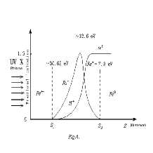
Figure 4: The schematic distributions of $Fe^{+}\leavevmode\nobreak\ and\leavevmode\nobreak\ H^{0}$ near the $H^{+}/H^{0}$ ionization front, i.e. the ionization structure of the surface layer of the cloud in BLR.

The special importance of the non-uniform plane-parallel slab is in that, according to the conventional photoionization model of BLR of AGNs, most low-ionized ions particularly the hydrogenic ions, e.g. $Fe^{+},Mg^{+},\cdots$, exist in a layer near to the ionization front of $H^{+}/H^{0}$, and have a non-uniform distribution, $N_{Fe^{+}}=N_{Fe^{+}}(s)$, $N_{Mg^{+}}=N_{Mg^{+}}(s),\cdots$. For example, it is known that the ionization thresholds of iron are $Fe^{0}/Fe^{+}/Fe^{++}=7.9/16.18/30.65{\rm eV}$, and the position of the front $H^{+}/H^{0}$ is at $\sim 13.6{\rm eV}$. So we infer that the low-ionized ions $Fe^{+}$ exist on both sides of the front $H^{+}/H^{0}$, where the density of neutral hydrogen $N_{H^{0}}$ varies drastically with $s$, $N_{H^{0}}=N_{H^{0}}(s)$, the same as the density of $Fe^{+},N_{Fe^{+}}=N_{Fe^{+}}(s)$. Fig. 4 shows the schematic distribution of $Fe^{+},H^{0},H^{+}$, in the neighbourhood of the front of $H^{+}/H^{0}\sim 13.6{\rm eV}$.

2.4.2 Extended formulae of intensity $I^{c}_{y}$ for complex atoms(ions) gas

For simplicity, we only give the formulae for the uniform and optically thick plane-parallel emission slab. The discussion is parallel to Sect. 2.4.1 for the hydrogenic atoms. Thus Eq. (31) is still valid for the heavy elements, only with a replacement of $N_{l}\rightarrow NS_{l}$ and $N_{u}\rightarrow NS_{u}$(Eq.($5^{\prime}$) in the expressions of $C_{0},C_{1},C_{2}$ in Eqs. (32), we then get the emergent intensity $I$ and the line profile for the Cerenkov line of the complex atoms(ions). Furthermore, in the optical waveband, the dominant absorber of photoionization is still hydrogen due to the great abundance of $H$, thus $k_{bf}$ is still given by the last equation in Eqs. (32).

However, if the Cerenkov line is located in the X-ray waveband, e.g. the Cerenkov Fe $K_{\alpha}$ line $\sim 6.4{\rm KeV}$, we must use the parameters $C_{0},C_{1},C_{2}$ and $k_{bf}$ given by Eq. ($20^{\prime}$), ($21^{\prime}$), $(24^{\prime\prime}$) and ($25^{\prime}$), ($25^{\prime\prime}$) respectively. For convenience, we relist all of these parameters in Eq. ($32^{\prime}$) below. Therefore, in Eq. (31),

$$y=\frac{\epsilon_{lu}-\epsilon}{\epsilon_{lu}}$$

$$C_{0}=1.05\times 10^{-76}\epsilon^{-4}_{lu}A_{ul}g_{u}N\left(\frac{S_{l}}{g_{l}}-\frac{S_{u}}{g_{u}}\right)$$

$$C_{1}=5.77\times 10^{-53}\epsilon^{-2}_{lu}A_{ul}g_{u}N\left(\frac{S_{l}}{g_{l}}-\frac{S_{u}}{g_{u}}\right)$$

$$C_{2}=1.75\times 10^{-87}\epsilon^{-4}_{lu}A_{ul}\Gamma_{lu}g_{u}N\left(\frac{S_{l}}{g_{l}}-\frac{S_{u}}{g_{u}}\right)\leavevmode\nobreak\ \leavevmode\nobreak\ \leavevmode\nobreak\ \leavevmode\nobreak\ \leavevmode\nobreak\ \leavevmode\nobreak\ \leavevmode\nobreak\ \leavevmode\nobreak\ \leavevmode\nobreak\ \leavevmode\nobreak\ (32^{\prime})$$

$$k_{bf}=8.4\times 10^{-46}\epsilon^{-3}_{lu}N(Fe)S_{2}\leavevmode\nobreak\ \leavevmode\nobreak\ \leavevmode\nobreak\ \leavevmode\nobreak\ \leavevmode\nobreak\ \leavevmode\nobreak\ \leavevmode\nobreak\ ({\rm for}\leavevmode\nobreak\ \leavevmode\nobreak\ \leavevmode\nobreak\ Fe\leavevmode\nobreak\ \leavevmode\nobreak\ K_{\alpha}-{\rm line})$$

and $\epsilon_{lu}$ is in unit ergs in CGSE system ($1{\rm KeV}=1.602\times 10^{-9}{\rm erg}$).

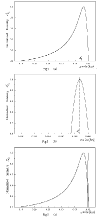
Figure 5: The emergent intensity $I^{c}_{\lambda}$ of $Fe^{+19}$ ions. (a) shows the line profile of $Fe^{+19}$ in gas of higher density $\gamma_{c}=1.0\times 10^{4}$, $N=2.5\times 10^{19}$; (b) shows a symmetric profile in gas of lower density $\gamma_{c}=1.0\times 10^{4}$, $N=2.5\times 10^{17}$; (c) combines the line-profiles of (a) and (b) for comparason.

Using Eq. (31), we calculated the Cerenkov $K_{\alpha}$ line $\sim 6.4{\rm KeV}$ of the iron ion $Fe^{+19}$, as shown in Fig. 5. The calculation parameters are chosen as $\gamma_{c}=1.0\times 10^{4}$, $N=2.5\times 10^{19}{\rm cm^{-3}}$(Fig.5 (a)) and $\gamma_{c}=1.0\times 10^{4}$, $N=2.5\times 10^{17}{\rm cm^{-3}}$ (Fig.5 (b)) respectively.

2.5 The Cerenkov line redshift $y^{c}_{t}$ (or $\Delta Z^{c}$)

2.5.1 Formulae of $y^{c}_{t}$ (or $\Delta Z^{c}$) for hydrogen or hydrogen-like gas

Using Eq. (31), the small “Cerenkov line redshift” $y^{c}_{t}$ can be obtained from the equation $\frac{dI^{c}_{y}}{dy}=0$. Thus we obtained:

$$\Delta Z^{c}\equiv y^{c}_{t}=\frac{\Delta\lambda^{c}_{t}}{\lambda_{lu}}=\frac{1}{y^{-1}_{\rm lim}+\sqrt{y^{-2}_{\rm lim}+\frac{k_{bf}}{C_{2}}}}$$

$$\leavevmode\nobreak\ \leavevmode\nobreak\ \leavevmode\nobreak\ =\frac{1}{C^{-1}_{0}\gamma^{-2}_{c}+\sqrt{C^{-2}_{0}\gamma^{-4}_{c}+\frac{k_{bf}}{C_{2}}}}$$ (38)

If the gas is very dense (e.g. $N_{H^{0}}\simeq 10^{16}{\rm cm^{-3}}$), we have a line width $y_{\rm lim}\gg\sqrt{C_{2}/k_{bf}}$ ($y_{\rm lim}\equiv\frac{\Delta\lambda^{c}_{\rm lim}}{\lambda_{lu}}\propto C_{0}\propto N$, but $C_{2}/k_{bf}$ is density-independent, see Eqs. (20), (32). Therefore from Eqs. (32) and (38) we get a simplified redshift formula:

$$\Delta Z^{c}\equiv y^{c}_{t}\simeq\sqrt{\frac{C_{2}}{k_{bf}}}$$

$$\leavevmode\nobreak\ \leavevmode\nobreak\ \leavevmode\nobreak\ =1.04\times 10^{-11}\sqrt{\lambda_{lu}A_{ul}\Gamma_{lu}\frac{g_{u}}{g_{l}}R_{l}R^{-1}_{p}p^{5}\xi}$$ (39)

where $\xi\equiv N/N_{H^{0}}$ represents the “abundance” of the concerned hydrogenic atom (ions) species. For the gas of neutral hydrogen $\xi=1$. It is easy to show that the wavelength displacement $y^{c}_{t}$ in Eq. (39) is just at the wavelength position where $k_{lu}=k_{bf}$. For the wavelength region $y\leq y^{c}_{t}$ which is close to $\lambda_{lu}$, we have $k_{lu}\gg k_{bf}$ which means that the Cerenkov line redshift is just caused by the great line absorption $k_{lu}$ at vicinity of $\lambda_{lu}$. From Eq. (39) we see, the redshift for the dense gas is $N$-independent, $\Delta Z^{c}$ is only dependent on the atomic parameters ($\lambda_{lu},A_{ul},\Gamma_{lu},\cdots$) and the temperature $T$ of the gas, and the “abundance” $\xi\equiv N/N_{H^{0}}$.

Another limiting case is for the gas with lower density, which makes $y_{\rm lim}\ll\sqrt{\frac{C_{2}}{k_{bf}}}$. In this case (but still optically thick for continuum, $k_{\lambda}L=(k_{lu}+k_{bf})L\gg 1)$), Eq. (38) is simplified as:

$$\Delta Z^{c}\equiv y^{c}_{t}\equiv\frac{\Delta\lambda^{c}_{t}}{\lambda_{lu}}\simeq\frac{y_{\rm lim}}{2}$$ (40)

where, $y_{\rm lim}$ is given by Eq. (20) ($y_{\rm lim}\propto N$). The critical point of “higher” and “lower” densities is determined by a critical equality $y_{\rm lim}=\sqrt{\frac{C_{2}}{k_{bf}}}$, from which we get a critical density $N^{cr.}$ of the concerned species in a gas:

$$N^{cr.}=1.54\times 10^{2}\left(\frac{g_{u}}{g_{l}}\right)^{-1/2}$$

$$\leavevmode\nobreak\ \leavevmode\nobreak\ \leavevmode\nobreak\ \times\gamma_{c}^{-2}\lambda^{-7/2}_{lu}A^{-1/2}_{ul}\Gamma^{1/2}_{lu}p^{5/2}(R_{l}R_{p})^{-1/2}\xi^{1/2}$$ (41)

Therefore, Eq. (39) and Eq. (40) are valid for $N\gg N^{cr.}$ and $N\ll N^{cr.}$ respectively. Fig. 3(c) shows the profile $I^{c}_{\lambda}\sim\Delta\lambda$ and the redshift $\Delta\lambda^{c}$ of the Cerenkov line for the case $N\gg N^{cr.}$. The red-asymmetry of the profile is remarkable. But for the cases $N\simeq N^{cr.}$ and $N\ll N^{cr.}$ (see Fig. 5 (b)), the profile becomes more symmetric. And the Cerenkov line redshift becomes very small.

We emphasize again, both Eq. (39) for $N\gg N^{cr.}$ and Eq. (40) for $N\ll N^{cr.}$ are derived from Eq. (31). Both Eq. (39) and Eq. (40) are valid only for the optically thick case, $\tau_{\lambda}=(k_{lu}+k_{bf})L\gg 1$.

2.5.2 Extended formulae of $y^{c}_{t}$ (or $\Delta Z^{c}$) for complex atoms (ions) gas

The formula of the Cerenkov line redshift, Eq. (38) is also valid for a gas composed of complex atoms (ions). The related parameters in (38), i.e. $C_{0},C_{1},C_{2}$ and $k_{bf}$ are still given by Eq. (32) only with replacement $\left(\frac{N_{l}}{g_{l}}-\frac{N_{u}}{g_{u}}\right)\Longrightarrow N\left(\frac{S_{l}}{g_{l}}-\frac{S_{u}}{g_{u}}\right)$, or equivalently, $N_{l}\rightarrow NS_{l}$, $N_{u}\rightarrow NS_{u}$(see Eq.($5^{\prime\prime}$), with unchanged $k_{bf}$ because the dominant photoionization absorber in the optical wavelength is still hydrogen.

In parallel, in the limiting cases, $y_{\rm lim}\gg\sqrt{\frac{C_{2}}{k_{bf}}}$ and $y_{\rm lim}\ll\sqrt{\frac{C_{2}}{k_{bf}}}$, or equivalently, $N\gg N^{cr.}$ and $N\ll N^{cr.}$, the simplified redshift formulae are still given by Eq. (39) and (40) respectively.

If the Cerenkov line of complex atoms or ions is in the X-ray band, it is better to change the wavelength in (32) into the photon energy, $\lambda_{lu}\rightarrow\epsilon_{lu}$, $\lambda_{lu}=\frac{hc}{\epsilon_{lu}}$, i.e. the parameters $C_{0},C_{2}$ and $k_{bf}$ in (38) have to be expressed by Eq. ($32^{\prime}$). given in Sect. 2.4.2, where $\epsilon_{lu}\equiv\epsilon_{u}-\epsilon_{l}=h\nu_{lu}$ is in unit ergs in the CGSE system, rather than KeV (1KeV=$1.602\times 10^{-9}{\rm ergs}$).

2.6 The emergent intensity $I^{c}$ of the Cerenkov line

2.6.1 Formulae of $I^{c}$ for hydrogen of hydrogen-like gas

Integrating Eq. (31), we obtained the total intensity $I^{c}$ of the Cerenkov line, for the optically thich uniform plane-parallel layer $I^{c}=\int_{0}^{y_{\rm lim}}I^{c}_{y}dy$ Thus

$$I^{c}=Y\left[\ln{(1+X^{2})}-2\left(1-\frac{\arctan{X}}{X}\right)\right]$$ (42)

where, $Y\equiv\frac{N_{e}}{2}\frac{C_{1}}{k_{bf}}$, $N_{e}$ is the density of relativistic electrons, $X\equiv\sqrt{\frac{k_{bf}}{C_{2}}}y_{\rm lim}$, $C_{0}$, $C_{1}$, $C_{2}$ and $k_{bf}$ are given by Eq. (32), $y_{\rm lim}$ is given by Eq. (20).

Eq. (42) is in principle valid for a uniform plane-parallel slab of emissive gas. But as an exception, it can be used to calculate the line intensity of the neutral hydrogen without any problem. Although the density of $H^{0}$ atoms, $N_{H^{0}}$ varies with depth $s$ drastically near the front $H^{+}/H^{0}$, $N_{H^{0}}=N_{H^{0}}(s)$, we point out that the ratio $(J^{c}_{\lambda}/k_{\lambda})_{H^{0}}$ is constant, despite the nonuniform ionization structure in the neighbourhood of the front $H^{+}/H^{0}$. Therefore $(J^{c}_{\lambda}/k_{\lambda})_{H^{0}}$ can be taken out of the integral $I^{c}_{\lambda}=\int_{0}^{\tau_{\lambda}(u)}e^{-\tau_{\lambda}}\left(\frac{J^{c}_{\lambda}}{k_{\lambda}}\right)d\tau_{\lambda}\simeq\frac{J^{c}_{\lambda}}{k_{\lambda}}$, which ensures the validity of Eq. (42).

For the non-uniform case, the low-ionization line, such as $Mg^{+},Fe^{+}$, $O^{+},\cdots$, the emergent intensity of Cerenkov line $I^{c}$, is also obtained from $I^{c}=\int_{0}^{y_{\rm lim}}I^{c}_{y}dy$, and $I^{c}_{y}$ is given by Eq. (35). The calculation is somewhat complicate. However, in the semi-quantitative estimation of $I^{c}$, we can still invoke Eq. (42) only regarding the factors $R_{l}\equiv N_{l}/N$, $R_{p}\equiv N_{H^{0}_{p}}/N_{H^{0}}$, particularly, $\xi\equiv N/N_{H^{0}}$ etc. as the average value $\overline{R_{l}},\overline{R_{p}},\overline{\xi},\cdots$, in the interval $(S_{1},S_{2})$, where the concerned atoms or ions exist.

2.6.2 Extended formulae of $I^{c}$ for complex atoms (ions ) gas

The emergent total intensity of Cerenkov line of the complex atoms (ions) in optically thick case is also given by Eq. (42), where $C_{0},C_{1},C_{2}$ and $k_{bf}$ are given by Eq. (32) replacing $N_{l}$ by $NS_{l}$ and $N_{u}$ by $NS_{u}$. Note that, when the Cerenkov line is in the X-ray band, Eq. ($32^{\prime}$) has to be used to replace Eq. (32).

3 Conclusion and Discussion

The Cerenkov line-like emission of the relativistic electrons, passing through an optically thick dense gas, which we suggested early in 1980, has been verified by elegant laboratory experiments (Xu et al. 1981, 1988, 1989). In this paper, we give a detailed and clearer physical discussion and emphasize the potential importance of this new mechanism for high-energy astrophysics, and give the extended and improved formula system describing the emergent intensity, the line profile, the line width and the Cerenkov redshift of the Cerenkov line, among which the extension of formulae to the multi-electron complex atoms(ions) has special significance for the study of the broad lines of heavy elements in AGNs, particularly for lines in the X-ray band.

A possible application of the new line emission mechanism is in the exploration of the origin of the broad $\sim 6.4{\rm KeV}$ $K_{\alpha}$ line of the low-ionized iron ions of Seyfert1 galaxies. Now the disk-line models, in which the $\sim 6.4{\rm KeV}$ $K_{\alpha}$ line is regarded as one of the reflection components from the disk, strongly illuminated by the hard X-ray continuum, are widely accepted to explain the origin and characters of the broad $K_{\alpha}$-line with asymmetric profile. It is believed that the “Compton reflection and iron fluorescence features”, provide a powerful probe of the accretion flow and the strong gravitational field (see e.g. Georgy & Fabian 1991; Reynolds, Fabian & Inoue 1995). However, people now question the relativistically smeared disk-line interpretation. According to the disk-line model, both the line profile and the position of the peak are dependent on the inclination angle $\theta$ of the disk, and therefore are different from one sample to anoth er. But the observations show similar profiles of the $K_{\alpha}$ line for all Seyfert1 galaxies, even for Seyfert2 galaxies, with nearly unchanged peak at $\sim 6.4{\rm KeV}$(Nandra, 1997,a,b), which implies that the $K_{\alpha}$ line might not be from the inner disk, as thought before. It seems more reasonable to replace the “old disk” by “cold cloudlets” and/or “cold filaments” around the central massive black hole. Furthermore, the line emission mechanism might not, or rather, not only be photoionization-fluorescence. The photoionization-fluorescence model predicts positive correlations of both the light curves and the fluxes between the $K_{\alpha}$ line and the X-ray continuum. But the observations do not confirm this (e.g. Lee et al. 1999). Besides, the p rediction of a marked absorption dip at edge $>7{\rm KeV}$ which always accompanies the fluorescent $\sim 6.4{\rm KeV}$ $K_{\alpha}$ line is also not confirmed by the observations(Young et al. 1998).

We have shown that fluorescence is not a ‘unique’ mechanism of the line-emission of the low-ionization iron in the X-ray band. Another line mechanism which can produce the $\sim 6.4{\rm KeV}$ $K_{\alpha}$ line is the Cerenkov line-like emission, as described in this paper. For a very dense gas, optically thick for the continuum, the Cerenkov line becomes the unique emission line which can escape from the surface of the cloud of dense gas. The Cerenkov line will be strong to match the observation when the density of relativistic electrons in BLR is high enough. Therefore this kind of line emission might be a new possible mechanism to attack the $6.4{\rm KeV}$ $K_{\alpha}$ problem of AGNs. We expect that some puzzles of $K_{\alpha}$ line of iron could be resolved in this way(e.g. the observed strange correlations of the light curves and the fluxes between the $K_{\alpha}$ line and X-ray continuum radiation), even though there remain a lot of problems to be solved.

References

• (1) Bethe H.A., Salpeter E.E., 1957, Encyclopedia of Physics, 35, 88
• (2) Cheng F.H., You J.H., Yan M., 1990, ApJ 358, 18
• (3) Georgy I.M., Fabian A.C., 1991, MNRAS 249, 352
• (4) Handbook of Physics, Condon E., Odishaw H., 1958, McGraw-Hill Company Inc., Chap. 6, 112
• (5) Lee J.C., Fabian A.C., Reynolds C.S., Brandt W.N., Iwasawa K., 1999, MNRAS 310, 973
• (6) Nandra K., George I.M., Mushotzky R.F. et al., 1997, ApJ 476, 70
• (7) Nandra K., George I.M., Mushotzky R.F. et al., 1997, ApJ 477, 602
• (8) Raynolds C.S., Fabian A.C., Inoue H., 1995, MNRAS 276, 1311
• (9) Tanaka Y. et al., 1995, Nat 375, 659
• (10) Turner T.J., George I.M., Nandra K. et al., 1997, ApJS 113, 23
• (11) Xu K.Z., Yang B.X., Xi F.Y., 1981, Phys. Lett. A86, 24
• (12) Xu K.Z., Yang B.X., Xi F.Y., 1988, Phys. Rev. A33, 2912
• (13) Xu K.Z., Yang B.X., Xi F.Y., 1989, Phys. Rev. A40, 5411
• (14) You J.H., Cheng F. H., 1980, Acta Phys. Sinica 29, 927
• (15) You H., Kiang T., Cheng F.H., Cheng F.Z., 1984, MNRAS, 211, 667
• (16) You J.H., Cheng F.H., 1987, ApJ, 332, 174
• (17) You J.H., Cheng F.H., Cheng F.Z., Kiang T., 1986, Phys. Rev. A34, 3015
• (18) Young A.J., Ross R.R., Fabian A.C., 1998, MNRAS 300, L11
Refer to caption