IONIZED GAS IN DAMPED Ly$\alpha$  PROTOGALAXIES: II. COMPARISON BETWEEN MODELS AND THE KINEMATIC DATA

Abstract

We test semi-analytic models for galaxy formation with accurate kinematic data of damped Ly$\alpha$ protogalaxies presented in a companion paper (Wolfe & Prochaska 2000). The models envisage centrifugally supported exponential disks at the centers of dark matter halos which are filled with ionized gas undergoing radial infall to the disks. The halo masses are drawn from cross-section weighted mass distributions predicted by CDM cosmogonies, or by the null hypothesis that the dark matter mass distribution has not evolved since $z$ $\sim$ 3 (i.e., the TF models). In our models C IV absorption lines detected in damped Ly$\alpha$ protogalaxies arise in infalling ionized clouds while the low ion absorption lines arise from neutral gas in the disks. Using Monte Carlo methods we find (a) The CDM models are incompatible with the low ion statistics at more than 99$\%$ confidence whereas some TF models cannot be ruled out at more than 88$\%$ confidence. (b) Both CDM and TF models are in general agreement with the observed distribution of C IV velocity widths. (c) The CDM models generate differences between the mean velocities of C IV and low ion profiles that are compatible with the data, while the TF model produces differences in the means that are too large. (d) Both CDM and TF models produce ratios of C IV to low ion velocity widths that are too large. (e) Neither CDM nor TF models generate C IV versus low ion cross-correlation functions compatible with the data.

While it is possible to select model parameters resulting in agreement between the models and the data, the fundamental problem is that the disk-halo configuration assumed in both cosmogonies does not produce significant overlap in velocity space between C IV and low ion velocity profiles. We conjecture that including angular momentum of the infalling clouds will increase the overlap between C IV and low ion profiles.

accepted by the Astrophysical Journal August 5, 2000

1 INTRODUCTION

This is the second of two papers which discuss ionized gas in damped Ly$\alpha$ systems. In Paper I (Wolfe & Prochaska 2000) we presented velocity profiles drawn from a sample of 35 damped Ly$\alpha$ systems for the high ions C IV and Si IV and the intermediate ion Al III. Comparison among these profiles and with profiles previously obtained for low ions such as Fe II showed the damped Ly$\alpha$ systems to consist of two distinct kinematic subsystems: a low ion subsystem composed of low and intermediate ions and a high ion subsystem containing only high ions. The evidence distinguishing between the kinematic subsystems is robust and stems from a battery of tests comparing distributions of various test statistics. It also stems from differences between the C IV versus low ion or C IV versus Al III cross-correlation functions on the one hand, and the C IV versus Si IV or Al III versus low ion cross correlation functions on the other. Whereas the latter have high amplitude and small velocity width, the former have lower amplitude and wider velocity width. This is because velocity profiles of ions arising in the same kinematic subsystem comprise narrow velocity components that line up in velocity space, whereas velocity components arising from ions in different kinematic subsystems are misaligned in velocity space. However, the existence of a statistically significant C IV versus low ion cross-correlation function suggests the two subsystems are interrelated. This is also indicated by a systematic effect in which the C IV profile velocity widths $\Delta v_{\rm CIV}$ are greater than or equal to the low ion profile velocity widths $\Delta v_{\rm low}$ in 29 out of 32 systems.

In Paper I we claimed these phenomena indicate that the two subsystems are located in the same gravitational potential well. In this paper we shall expand on this idea with specific models. The models assume that the low ion subsystems are centrifugally supported disks of neutral gas located at the centers of dark matter halos (see Mo et al.  1998; hereafter referred to as MMW), whereas the high ion subsystems comprise photoionized clouds undergoing infall from a gaseous halo to the disk. That is, we assume the dark matter halos contain hot virialized gas in pressure equilibrium with the photoionized clouds. The hot gas undergoes a subsonic cooling flow toward the disk while the denser clouds infall at velocities approaching free fall (Mo & Miralda-Escud$\rm\acute{e}$ 1996; hereafter referred to as MM). The models are set in a cosmological context by computing the mass distribution and other properties of the dark matter halos using Press-Schecter theory and the CDM cosmogonies adopted by semi-analytic models for galaxy formation. We also consider the null hypothesis that galaxies at $z$ $\approx$ 3 have the same dynamical properties of nearby galaxies (this model, hereafter referred to as the TF model, is defined in $\S$ 2.4.2).

We test the models using a Monte Carlo technique for computing absorption spectra arising when sightlines that randomly penetrate intervening disks also intercept ionized clouds in the halo. $\S$ 2 presents models for the neutral gas. We discuss properties of the disk, the cosmological framework, and Monte Carlo techniques. In $\S$ 3 we discuss models for the ionized gas. We derive expressions for the structure and kinematics of the two-phase halo gas. Expressions for C IV column densities of the clouds are derived. In $\S$ 4 we give results of the Monte Carlo simulations for the low ion gas for both CDM and TF model. Results of Monte Carlo simulations for the ionized gas are given in $\S$ 5. Here we also consider tests of correlations between the kinematics of the high ions and low ions. In $\S$ 6 we investigate how the results of $\S$ 5 are affected by changes in some key parameters such as central column density and low end cutoff to the input dark-matter halo mass distribution. Concluding remarks are given in $\S$ 7.

2 MODELS OF THE NEUTRAL GAS

2.1 Cosmological Framework

To place the model in a cosmological context we assume bound dark-matter halos evolve from linear density contrasts, $\delta(x,t)$$\equiv$$\delta\rho/\rho$, according to gravitational instability theory for Friedmann cosmologies (Peebles, 1980). We consider adiabatic CDM models (ACDM) in which $\delta_{k}$, the Fourier transforms of $\delta(x,t)$, are Gaussian distributed with variance given by $P(k)$, the power spectrum at the epoch of radiation and matter equality. We also consider isocurvature CDM models (ICDM) in which the $\delta_{k}$ are not Gaussian distributed (Peebles, 1999b). The $\delta_{k}$, or more specifically the rms density contrasts in spheres with mass scale $M$, i.e., $\Delta_{M}$, grow with time until they go non-linear and collapse. According to the spherical collapse model, this occurs when the $\Delta_{M}$ predicted by linear theory equals $\delta_{c}$ = 1.68. To compute $n(M,z)dM$, the density of bound halos in the mass interval ($M$, $M$$+$$dM$), we follow previous authors (e.g. MMW) who used the Press-Schecter formalism in the case of ACDM. In Appendix A we derive an expression for $n(M,z)dM$ in the case of ICDM.

We shall also test the null hypothesis that little or no evolution of galaxies has occurred since the epochs of damped Ly$\alpha$ absorption; that is, an hypothesis assuming current disks, with higher ratios of gas to stars, were in place at $z$ $>$ 3. This scenario resembles the semi-analytic models in that we assume centrifugally supported disks reside at the centers of dark matter halos filled with hot gas at the virial temperatures. However, we do not assume a CDM power spectrum nor the Press-Schecter formalism to compute the mass distribution of halos. Rather, we assume (a) the luminosity function of galaxies in the redshift range of the damped Ly$\alpha$ sample in paper I, i.e., $z$ = [2,5], is given by the Schecter function determined from nearby galaxies (e.g. Loveday et al.  1999), (b) galaxies at these redshifts obey the same Tully-Fisher relationship between luminosity and rotation speed as at $z$ = 0, and (c) a correlation between disk radial scale-length and disk rotation speed exists. This model, hereafter referred to as TF, is an extension of the rapidly rotating disk model suggested by Prochaska & Wolfe (1997 and 1998; hereafter PW1 and PW2). We describe this model in more detail in the following sections

Throughout the paper we shall intercompare results for the TF model and four CDM cosmogonies. The cosmological settings of the CDM models are specified by (i) the current total matter density, $\Omega_{M}$, (ii) the cosmological constant, $\Omega_{\Lambda}$, (iii) the Hubble constant, $h$, where $h$ = $H_{0}$/ 100 km s^-1 Mpc^-1, (iv) $\sigma_{8}$, the rms linear density contrast at $z$ = 0 in spheres of radius 8$h^{-1}$ Mpc, and (v) $n$, the power-law index for the power spectrum, in cases where $P(k)$ $\propto$ $k^{n}$. The values of the parameters are given in Table 1. The SCDM, $\Lambda$CDM, and OCDM are normal ACDM models. In all three cases, $P(k)$ is given by the Bardeen et al. (1986) expression (which is not a power law). In the ICDM model we follow Peebles by assuming $P(k)$ $\propto$ $k^{n}$ and $n$ = $-$1.8. The cosmological parameters specifying the TF model are also given in Table 1.

2.2 Disk Models

Most semi-analytic models assume the neutral gas causing damped Ly$\alpha$ absorption is confined to centrifugally supported disks at the centers of dark-matter halos (e.g., Kauffmann 1996; MMW). The spherical collapse model is used to define the limiting virial radius as $r_{200}$, the radius within which the mean density of dark matter equals 200$\rho_{crit}(z)$ where $\rho_{crit}(z)$ is the critical density of the universe at redshift $z$. Thus, $V_{200}$, the circular velocity at $r_{200}$, is related to $r_{200}$ and $M$, the halo mass within $r_{200}$, by

$$V_{200}=[10GH(z)M]^{1/3};\ r_{200}={V_{200}\over{10H(z)}}\;\;\;,$$ (1)

where $H(z)$ is the Hubble parameter, ($a^{-1}da/dt$), at $z$. MMW also define $m_{d}$ and $j_{d}$ as the fractions of halo mass, $M$, and angular momentum, $J$, in disk baryons. Assuming the halos to be singular isothermal spheres embedding disks having exponential surface-density profiles with radial scale-lengths, $R{{}_{d}}^{iso}$, they find that

$$R_{d}^{iso}={1\over\sqrt{2}}{j_{d}\over m_{d}}{\lambda}{r_{200}}\approx 8.8\ h^{-1}{\rm kpc}{\Bigg{(}}{\lambda\over 0.05}{\Bigg{)}}{}$$

$${\times}{\Bigg{(}}{V_{200}\over{250{\rm kms^{-1}}}}{\Bigg{)}}{\Bigg{[}}{H(z)\over H_{0}}{\Bigg{]}^{-1}}{\Bigg{(}}{j_{d}\over m_{d}}{\Bigg{)}}\;\;\;,$$ (2)

and

$$N_{0}^{iso}=4.8{\times}10^{22}h\ {\rm cm^{-2}}{\Bigg{(}}{m_{d}\over 0.05}{\Bigg{)}}{\Bigg{(}}{\lambda\over 0.05}{\Bigg{)}^{-2}}{}$$

$${\times}{\Bigg{(}}{V_{200}\over{250{\rm kms^{-1}}}}{\Bigg{)}}{\Bigg{[}}{H(z)\over H_{0}}{\Bigg{]}}{\Bigg{(}}{m_{d}\over j_{d}}{\Bigg{)}^{2}}\;\;\;,$$ (3)

where the spin parameter of the halo, $\lambda$ = $J|E|^{1/2}G^{-1}M^{-5/2}$, ($E$ is the total energy of the halo) and $N_{0}$ is the central H I column density perpendicular to the disk. The distribution of $\lambda$ is given by

$$p({\lambda})d{\lambda}={1\over{\sqrt{2\pi}}\sigma_{\lambda}}{\rm exp}{\Bigg{[}}-{{\rm ln}^{2}({\lambda/<\lambda>})\over 2\sigma_{\lambda}^{2}}{\Bigg{]}}{d{\lambda}\over{\lambda}}\;\;\;,$$ (4)

where the mean and dispersion are determined from numerical simulations to be $<\lambda>$ = 0.05 and $\sigma_{\lambda}$ =0.5 (see Barnes & Efstathiou 1987).

For the TF models we infer the parameters of the halo from observed properties of the disk. Thus, we use model rotation curves to infer $V_{200}$ from $V_{max}$, the observed maximum rotation speed (see below). We then use eq. (1) to obtain the mass and virial radius of the halo. In this case we obtain the radial scalelength and central column density of the disk by adopting the following correlations inferred by MMW from the spiral galaxy data of Courteau (1996; 1997):

$$R_{d}^{Cor}=-1.25+7.4(V_{max}/250{\rm kms}^{-1})\ h^{-1}\ {\rm kpc}\;\;\;,$$ (5)

$$N_{0}^{Cor}=3.6{\times}10^{22+0.45(V_{max}/250{\rm kms}^{-1})}{\mu}^{-1}\ h\ {\rm cm}^{-2}\;\;\;,$$ (6)

where $\mu$ is the mean molecular weight of the gas.

2.3 Rotation Curves

We next turn to the mass distribution of the halo. This is crucial for determining both the rotation curve of the disk and the dynamics of gaseous infall discussed in $\S$ 3. For our model we adopt the analytical fit to the halo mass distribution found in the N-body simulations of Navarro et al.  (1997; hereafter NFW). In this case the halo rotation curve, defined by $V_{rot}(r){\equiv}\sqrt{GM(r)/r}$, has the following form:

$$V_{rot}(r)=V_{200}{\sqrt{{c\over x}{{{\rm ln}(1+x)-x/(1+x)}\over{\rm ln}(1+c)-c/(1+c)}}}\;\;\;;x=r/r_{s}\;\;\;,$$ (7)

where the concentration parameter, $c\equiv r_{200}/r_{s}$, and at $r$ = $r_{s}$, the halo mass density $\rho\propto r^{-2}$. NFW developed a self-consistent theory in which $c$ depends on $V_{200}$ and redshift, $z$, in the sense that at a given $z$, $c$ declines with increasing $V_{200}$, and at a given $V_{200}$, c decreases with $z$. We use the algorithms described in Navarro et al.  (1997) to compute $c$=$c(z,V_{200})$. NFW halo rotation curves corresponding to $z$ = 2.5, $\lambda$ = 0.05, $m$ = 0.05, and the ${\Lambda}$CDM cosmology appear as solid curves in Figure 1 for $V_{200}$ = 50$-$250 km s^-1 . As expected $V_{rot}$ = $V_{max}$ at $r$ $\approx\ 2r_{s}$. Curves with lower $V_{200}$ appear to rise more rapidly in the interval $r$ = [0,$r_{200}$] because the ratio $r_{s}$/$r_{200}$ decreases with decreasing $V_{200}$.

However, the expression for the halo $V_{rot}(r)$ in eq. (7) is incomplete as it ignores the presence of the disk. Self-gravity of the disk affects the mass distribution of the halo through adiabatic contraction (Blumenthal et al.  1984). We used the MMW formalism to compute rotation curves due to contracted halos and found that $V_{rot}(r)$ differed from the expression in eq. (7) by less than $\approx$ 15$\%$. Given the uncertainties in the models we shall ignore these corrections and use the halo mass distribution implied by eq. (7) when computing dynamics of infall.

On the other hand the rotation curve of the disk can differ significantly from eq. (7) when the disk contribution to the net potential gradient is added to that of the contracted halo. MMW compute the scale length and central column density of centrifugally supported exponential disks in adiabatically contracted NFW halos formed by spherical collapse. In comparison with halos modeled as singular isothermal spheres they find

$$R^{MMW}_{d}={R_{d}^{iso}}{f_{c}^{-1/2}}f_{R}\;\;\;,N^{MMW}_{0}={N_{0}^{iso}}f_{c}f_{R}^{-2}\;\;\;.$$ (8)

Explicit expressions for the functions $f_{c}$ and $f_{R}$ are given by MMW. They then use the new disk parameters to calculate the modified $V_{rot}(r)$ for disks embedded in NFW halos. Examples of modified $V_{rot}(r)$ corresponding to $\lambda$ = 0.05, $m_{d}$ = 0.05, and $z$ = 2.5 are shown as dotted curves in Figure 1. Clearly the rotation speeds sampled by sightlines traversing these model disks lie between $V_{200}$ and $f_{V}$$V_{200}$, the maximum of the modified disk rotation curve, where $f_{V}$, a function tabulated by MMW, exceeds unity. Given the wide range of possible rotation curves appropriate for model damped Ly$\alpha$ systems (see PW2), we assume that the disk rotation curves have either of the following constant speeds:

$$V_{rot}(r)=V_{200}{\times}\left\{\begin{array}[]{ll}1\\ f_{V}\ \;\;\;.\end{array}\right.$$ (9)

Figure 1: NFW rotation curves corresponding to $z$ = 2.5, $\lambda$ =0.05, $m$ = 0.05 and the $\Lambda$CDM cosmology. Solid curves are halo rotation curves from eq. (9) corresponding to $V_{200}$ = 50, 100, 150, 200, and 150 km s^-1 . Dotted curves show rotation curves resulting from modifications due to adiabatic contraction and disk self-gravity. Curves plotted out to $r_{200}$

For the TF models $V_{200}$ is not given apriori. Rather we assume $V_{rot}(r)$ = $V_{max}$ and that $V_{max}$ is selected from an empirical distribution derived from the Tully-Fisher relation (see $\S$ 2.4.2). The radial scale length and central column densities then follow from eqs. (5) and (6). In this case $V_{200}$ = $V_{max}$ or $V_{200}$ =$V_{max}$/$f_{V}$.

2.4 Monte Carlo Models

In previous work (PW1, PW2) we tested models by comparing predicted and empirical distributions of the four test statistics for the low ions (Figure 6 in Paper I). The model distributions were computed by a Monte Carlo technique in which low ion absorption profiles were produced by sightlines traversing 10000 randomly oriented disks, and test statistics were determined for each profile. In PW1 the disk models were based on the simplifying assumption of identical disks with flat rotation curves characterized by a single rotation speed, while in PW2 more realistic forms of $V_{rot}(r)$ were used for the identical disks. Here we extend this approach to account for the distributions of halo masses and spin parameters.

2.4.1 CDM

MMW give an expression for the cumulative probability that sightlines to the background QSOs intercept disks in halos with masses exceeding that corresponding to $V_{max}$: the result is averaged over $p(\lambda)$. For the Monte Carlo model we require the differential expression; that is, the probability for intercepting disks in the spin parameter interval ($\lambda,\ \lambda+d\lambda$), circular velocity interval ($V_{200},\ V_{200}+dV_{200}$), and redshift interval ($z,\ z+dz$). The result is given by

$$dP_{CDM}(z,{\lambda},V_{200})=\Bigl{[}dz{{\pi}\over 2}(1+z)^{3}\bigl{(}-c{dt\over dz}\bigr{)}\Bigr{]}$$

$$\times d\lambda p(\lambda)\Bigl{[}R_{d}^{iso}(V_{200},\lambda,z)N_{0}^{iso}(V_{200},\lambda,z)\Bigr{]}^{2}$$

$$\times dV_{200}n(V_{200},z)F(N_{0}^{iso})\;\;\;,$$ (10)

where

$$F(N_{0}^{iso})=\left\{\begin{array}[]{ll}{1\over(N_{0}^{iso})^{2}}{\Biggl{[}}{1\over 2}+{\rm ln}(N_{0}^{iso}/N_{l}){\Bigl{(}}1+{\rm ln}(N_{0}^{iso}/N_{l}){\Bigr{)}}{\Biggr{]}}\ ;\\ N_{0}^{iso}>N_{l},\\ {1\over 2N_{l}^{2}}\ ;N_{0}^{iso}<N_{l},\end{array}\right.$$ (11)

and

$$n(V_{200},z)=n(M,z){\Biggl{|}}{dM\over dV_{200}}{\Biggr{|}}\;\;\;.$$ (12)

Here $N_{l}$ = $2{\times}10^{20}$cm^-2 is the threshold column density for damped Ly$\alpha$ surveys (e.g. Wolfe et al.  1995).

Figure 2: Input circular velocity distributions for the CDM and TF models used in Monte Carlo simulations. Computed as described in the text for the velocity interval (30, 300) km s^-1 . The abscissa correspond to $V_{200}$ in CDM and $V_{max}$ in TF models.

For given redshift intervals and cosmologies, the function $dP_{CDM}$ describes a surface above the ($\lambda$, $V_{200}$) plane. To form synthetic samples of 10000 low ion profiles, we randomly draw ($\lambda$, $V_{200}$) pairs according to the height of the surface above the plane. To assure compliance with the damped Ly$\alpha$ surveys, sightlines resulting in observed H I column densities less than $N_{l}$ are thrown out. We restrict the boundaries of the surface to $V_{200}\ <$ 300 km s^-1 to insure that gas in virialized halos has ample time to cool and collapse to the disk (e.g. Rees & Ostriker 1977) by a redshift, $z$ = 2.6, the median redshift of the kinematic sample. We also assume $dP_{CDM}$ cuts off below $V_{200}$ = 30 km s^-1 since gas photoionized to temperatures of $\sim$ 10⁴ K by the UV background radiation escapes from the dark matter halos with $V_{200}$ $<$ 30 km s^-1 (Thoul & Weinberg 1995; Navarro & Steinmetz 1997; Kepner et al.  1997: we investigate the consequences of modifying this restriction in $\S$ 6). Figure 2 shows the resulting distributions of $V_{200}$ for all the CDM models in Table 1. All the CDM curves exhibit maxima near the $V_{200}$ cutoff predicted by hierarchical cosmologies, and as predicted the curves decline with increasing $V_{200}$. As expected the largest fraction of massive halos is indicated for the ICDM models. Thereafter, the fraction decreases progressively from OCDM, $\Lambda$CDM, to SCDM adiabatic models.

Table 1: Model Parameters

MODEL	SCDM	$\Lambda$CDM	OCDM	ICDM	TF
$\Omega_{M}$	1.0	0.3	0.2	0.2	0.3
$\Omega_{\Lambda}$	0.0	0.7	0.0	0.8	0.7
$h$	0.5	0.7	0.7	0.7	0.7
$\sigma_{8}$	0.6	1.0	1.03	0.9	…
$n$				$-$1.8	…

2.4.2 TF

The curve labeled TF in Figure 2 represents the null hypothesis discussed above. In this case the x-axis corresponds to $V_{max}$ rather than $V_{200}$. This is because $V_{200}$ is a theoretical construct, whereas the null hypothesis is based only on the observed properties of current galaxies. The crucial relation ship here is the Tully-Fisher equation which connects $L$ and $V_{max}$; i.e.,

$$L(V_{max})=L_{*}(V_{max}/V_{*})^{\gamma}\;\;\;,$$ (13)

where $V_{*}$ is $V_{max}$ for a galaxy with luminosity $L$ = $L_{*}$. With the last equation we can obtain expressions for the interception probability

$$dP_{TF}(z,V_{max})=\Bigl{[}dz{\pi\over 2}(1+z)^{3}\bigl{(}-c{dt\over dz}\bigr{)}\Bigr{]}$$

$$\times\Bigl{[}R_{d}^{Cor}(V_{max},z)N_{0}^{Cor}(V_{max},z)\Bigr{]}^{2}$$

$$\times dV_{max}n(V_{max},z)F(N_{0}^{Cor})\;\;\;,$$ (14)

where d$V_{max}$$n[L(V_{max})]$ is the present density of galaxies with maximum rotation velocities in the interval ($V_{max}$, $V_{max}$$+$d$V_{max}$), and $F(N_{0}^{Cor})$ is given by eq. (11) with $N_{0}^{Cor}$ substituted for $N_{0}^{iso}$. To determine $n[L(V_{max})]$ we assume a Schecter luminosity function; i.e.,

$$dV_{max}n(V_{max},z)={\Phi_{*}}({L/L_{*}})^{-\alpha}{\rm exp}(-L/L_{*})d(L/L_{*})\;\;\;.$$ (15)

The TF curve depends on the parameters $\alpha$, $\gamma$, and $V_{*}$ for which we assumed values of 1.0, 3.0, and 250 km s^-1 respectively. These are representative for the values of parameters adopted by Gonzalez et al. (2000) who computed $n$($V_{max}$,0). They analyzed data sets from extensive surveys carried out at $B$ magnitudes. However, using Cepheid calibrated galaxies Sakai et al. (2000) derive Tully Fisher relations indicating lower values of $V_{*}$ ($\approx$ 180 km s^-1 ) for the $B$ magnitude Tully Fisher relation. Low values of $V_{*}$, as well as higher values of $\gamma$, are indicated by their $I$ band Tully Fisher relation, and from similar relations found by Giovanelli et al. (1997). In $\S$ 6 we discuss the sensitivity of our results to these parameters . The point we wish to emphasize is that for acceptable ranges of these parameters the TF curve differs from the CDM curves in that it (a) peaks at $V_{max}$ $\approx$ $V_{*}$/2 $\approx$ 130 km s^-1 , which is large compared to the 30 km s^-1 peak of the CDM curves, (b) has little power near the latter peak, and (c) falls off exponentially when $V_{200}$ $>$ $V_{*}$/2. Of course the comparison with CDM is inexact since $P_{CDM}$ depends on $V_{200}$ while $P_{TF}$ depends on $V_{max}$. Still the differences between $V_{200}$ and $V_{max}$ are not large enough to invalidate these conclusions.

3 IONIZED GAS

Assume that disks arise from the infall of ionized gas predicted to fill dark-matter halos. According to the MM model the halo gas is accreted during merger events with other halos and is shock-heated to the virial temperature of the halo, $k{T_{vir}}$ $\equiv$ (1/2)(${\mu}m_{H}$$V_{200}^{2}$); we assume $\mu$ = 0.4. The duration of the accretion phase is presumably short compared to $t_{M}$, the time-interval between events. For the mass interval corresponding to $V_{200}$ = [30, 300] km s^-1 , $T_{vir}$ ranges between 3$\times$10⁴ and 3$\times$10⁶K. In the case of massive halos the cooling time, $t_{cool}$, exceeds the age of the gas, $t_{M}$, at $r$ = $r_{200}$. Because the density of the gas increases with decreasing radius, $t_{cool}$ decreases with decreasing radius until $t_{cool}$ = $t_{M}$ at the cooling radius, $r_{cool}$. At $r\ <$ $r_{cool}$ the gas moves radially inward in a quasistatic cooling flow (Fabian, 1994). Cool clouds form in pressure equilibrium with the hot gas since the hot gas is thermally unstable. Due to the loss of buoyancy, the denser clouds fall inward at speeds determined by the imbalance between gravity and ram pressure. Because of rapid cooling, most of the gas in lower mass halos cools before moving inward, but within a limited range of halo masses there is always hot low-density gas left over which also moves inward in a cooling flow and exerts pressure on cooler clouds which have formed. The MM hypothesis is that the cool clouds are photoionized by background UV radiation and that they are the sites of C IV absorption lines in QSO absorption systems. Here we extend this hypothesis to model the ionized gas causing C IV absorption in damped Ly$\alpha$ systems.

Figure 3: Solid curves are pressure profiles for hot gas in halos with $V_{200}$ = 100 and 250 km s^-1 in (a) and (b) respectively. Pressure profiles are given by product of ${\rho(r)}_{h}$ and $T_{h}(r)$, the density and temperat ure of the hot gas. Profiles computed according to prescription in Appendix B. Dot-dashed curves are smooth density of cool gas times temperature of clouds; i.e. ${\rho}_{c}$$T_{cld}$. When latter exceeds pressure of hot gas, presure equilibrium between cool clouds and hot gas breaks down (see $\S$ 4.1)

3.1 Two Phase Structure of the Halo Gas

Following MM we assume the hot gas is in hydrostatic equilibrium with the dark matter potential and that it exhibits adiabatic temperature and density profiles out to $r_{min}$ = min($r_{cool}$,$r_{200}$). At $r\ >r_{min}$ the hot gas either follows isothermal profiles when $r_{200}$ $>$ $r_{cool}$ or does not exist when $r_{200}$ $<$ $r_{cool}$. In Appendix B we derive expressions for $r_{cool}$, and for $\rho_{h}(r)$ and $T_{h}(r)$, the density and temperature profiles for hot gas in halos corresponding to the unmodified NFW rotation curves in eq. (7). Examples of pressure profiles for high and low mass halos are shown in Figure 3 . The Figure shows the gas pressure in high mass halos to be 10 to 100 times higher than in low mass halos. The high pressures are mainly due to the higher virial temperatures of massive halos.

Gas in the cool phase comprises identical uniform spherical clouds with mass, $M_{cld}$, radius, $R_{cld}$, temperature, $T_{cld}$, and internal density, $\rho_{int}$. We adopt the MM model by assuming clouds form at $r=r_{min}$ with mass $M_{cld}(r_{min})$ = 4$\times$10⁵ $M_{\odot}$, and temperature, $T_{cld}$ =2$\times$10⁴K, since they are assumed to be photoionized. To compute $R_{cld}$, MM assume $\rho_{int}$ is set by pressure equilibrium with the surrounding hot gas; i.e., $\rho_{int}$ = ${\rho_{h}}T_{h}/T_{cld}$. But this assumption is incorrect for a wide range of halo masses and radii. Specifically, pressure equilibrium breaks down when the pressure is sufficiently low for $R_{cld}$ to equal the mean distance separating clouds. This will occur when $\rho_{c}(r)$, the average density of cool gas, exceeds $\rho_{int}(r)$; i.e., when ${\rho_{c}}{T_{cld}}$ $>$ ${\rho_{h}}{T_{h}}$. According to MM, $\rho_{c}(r)$ is given by

$${\rho_{c}(r)}={C_{1}\over r^{2}}\ ,$$ (16)

where the constant $C_{1}$ is evaluated in Appendix C. Figure 3 demonstrates how $r_{cross}$, the radius at which ${\rho_{c}}{T_{cld}}$ = ${\rho_{h}}{T_{h}}$, decreases with increasing $V_{200}$. In Figure 4 we plot $r_{cross}$, $r_{cool}$, and $r_{200}$ versus $V_{200}$ for a ${\Lambda}$CDM cosmology, NFW halos, and $z$ = 2.5 (we also plot the cooling radius of a singular isothermal sphere, $R_{cool}$, for comparison with NFW halos). The point of the Figure is to show that (1) pressure equilibrium breaks down throughout halos with $V_{200}$ $<$ 100 km s^-1 , (2) pressure equilibrium breaks down only near the centers of halos with $V_{200}$ $>$ 100 km s^-1 , (3) $r_{min}$ = $r_{200}$ for halos with $V_{200}$ $<$ 250 km s^-1 , and (4) $r_{min}$ = $r_{cool}$ for halos with $V_{200}$ $>$ 250 km s^-1 . These trends are qualitatively similar for all the background cosmologies in Table 1.

Figure 4: Critical radii versus $V_{200}$ for $\Lambda$CDM cosmology, NFW halos, and $z$ = 2.5. $R_{cool}$, the cooling radius of an infinite isothermal sphere is computed from eq. (B7), and $r_{cool}$ the cooling radius of an NFW halo is computed from eq. (B6). The ”virial radius” $r_{200}$ is computed from eq. (3). The crossing radius $r_{cross}$, computed from eq. (C8), is the radius within which pressure equilibrium breaks down. Note $r_{min}$ = min($r_{200}$,$r_{cool}$) for values of $V_{200}$ where $r_{cross}$ $\leq$ $r_{200}$. At $V_{200}$ $<$ 100 km s^-1 , $r_{min}$ = $r_{cross}$ = $r_{200}$ (see $\S$ 4.2).

In order to compute the structure of the cool clouds we assume ${\rho_{int}}$ = ${\rho_{c}}$ at $r\ <r_{cross}$. As a result

$$\rho_{int}(r)=\left\{\begin{array}[]{ll}{{\rho_{h}(r)}T_{h}(r)\over T_{c}}\ ;r>r_{cross}\\ {\rho_{c}(r)}\ ;r<r_{cross}\;\;\;.\end{array}\right.$$ (17)

The cross-section of the infalling clouds is then given by

$$A(r)={\pi}{\Biggl{(}}{3M_{cld}(r)\over 4{\pi}}{\Biggl{)}}^{2/3}\left\{\begin{array}[]{ll}({T_{c}\over{T_{h}(r){\rho_{h}(r)}}})^{2/3}\ :r>r_{cross}\\ ({1\over{\rho_{c}(r)}})^{2/3}\ ;r<r_{cross},\end{array}\right.$$ (18)

which will be smaller than the value computed from pressure equilibrium at $r\ <r_{cross}$. At $r\ >r_{cross}$, $M_{cld}$ is assumed to be a function of $r$ as the clouds may sweep up hot gas as they fall inward (see Benjamin & Danly 1997 for a discussion of this problem). At $r\ <r_{cross}$ the density of hot gas is negligible, and so we assume $M_{cld}(r)$ = $M_{cld}(r_{cross})$. Therefore we compute $M_{cld}(r)$ by solving

$${dM_{cld}\over dr}=\left\{\begin{array}[]{ll}-A(r){\rho_{h}(r)}\ ;r>r_{cross}\\ 0\ ;r<r_{cross},\end{array}\right.$$ (19)

subject to the boundary value of $M_{cld}(r_{cross})$. Explicit expressions for $A(r)$ and $M_{cld}(r)$ are given in Appendix C.

3.2 Cloud Kinematics

The hot gas surrounding the clouds will exert a drag force opposing their radial infall. Assuming the drag is caused by momentum imparted to the clouds by hot gas swept up during infall, we find the radial equation of motion to be

$${d\over dt}{\Bigl{[}}M_{cld}V_{r}{\Bigr{]}}=M_{cld}g(r)\;\;\;,$$ (20)

where $g(r)$ is the gravitational acceleration and the radial velocity, $V_{r}=-dr/dt$, is positive for infalling bodies. It follows that

$${dV^{2}_{r}\over dr}+{\Bigl{(}}{d{\rm ln}M_{cld}^{2}\over dr}{\Bigr{)}}V^{2}_{r}=-2g(r)\;\;\;,$$ (21)

(which corresponds to the case $C_{D}$ = 2 of Benjamin & Danly [1997]). The solution to equation (21) is

$$V^{2}_{r}(r)={2\over M^{2}_{cld}(r)}{\int_{r}^{r_{start}}dr^{{}^{\prime}}g(r^{{}^{\prime}})M^{2}_{cld}(r^{{}^{\prime}})}+V_{r}^{2}(r_{start})\;\;\;,$$ (22)

where we have computed the radial velocity of a cloud that starts to infall from an initial radius, $r$=$r_{start}$, with an initial velocity, $V_{r}(r_{start})$. Note, this expression ignores fragmentation of the clouds due to Kelvin-Helmholtz instabilities which may be important (Lin & Murray, 2000).

To compute $V_{r}(r)$ we assume the clouds infall from rest at $r$=$r_{min}$. As a result we solve eq. (22) with $r_{start}=r_{min}$ and $V_{r}(r_{start})$ = 0. The resultant $V_{r}(r)$ are valid in the interval $r$=[$r_{cross}$,$r_{min}$]. The solution for $V_{r}(r_{cross})$ acts as boundary condition in the first of two scenarios we consider for obtaining $V_{r}(r)$ at $r\ <r_{cross}$.

In the first scenario, clouds at $r$$<$$r_{cross}$ follow pressure-free ballistic trajectories along which $M_{cld}(r)$=const. In halos with $r_{cross}$ less than $r_{min}$ we solve eq. (22) by assuming $r_{start}=r_{cross}$ and let $V_{r}(r_{start})$ equal the $V_{r}(r_{cross})$ obtained from the solution at $r$ $>$ $r_{cross}$. For halos with $r_{cross}$ greater than $r_{min}$ we solve eq. (22) by assuming $r_{start}=r_{min}$ and $V_{r}(r_{start})$=0; i.e., the clouds undergo ballistic infall from rest at $r$=$r_{min}$.

In the second scenario we assume the cloud kinematics at $r$ $<$ $r_{cross}$ are dominated by random motions. These may be generated by feedback from supernova remnants arising from star formation stimulated in cloud-cloud collisions. Such scenarios have been suggested to solve the “cooling catastrophe” characterizing the hierarchical build up of galaxy-scale structure in most CDM models (White & Frenk, 1991). We obtain the velocity dispersion of the clouds by solving the Jeans equations for ${\sigma_{r}}$, the radial velocity dispersion for a system of clouds with (i) an isotropic velocity distribution, (ii) an average density distribution given by $\rho_{c}(r)$, and (iii) the gravitational field of an NFW halo (see eq. D4 in Appendix D). We then randomly draw the velocities of individual clouds from a Gaussian velocity distribution with dispersion given by $\sigma_{r}$.

We emphasize that our model is most uncertain for low mass halos. This is because the underlying assumption of pressure equilibrium, which allowed MM to compute the properties of the clouds, breaks down throughout the infalling gas for halos with $V_{200}$ $<$ 100 km s^-1 . In these halos the properties of individual clouds are difficult to compute because without a confining medium the clouds become indistinguishable at $r$ $<$ $r_{cross}$. Our approach to this problem is to assume the line of sight traverses a medium containing “cloud-like” structures with fixed masses and that these give rise to C IV absorption lines. This assumption needs to tested with high-resolution hydrodynamical simulations of gas at $r$ $<$ $r_{cross}$ which is subject to input of mechanical energy. We have also assumed eq. (17) is valid to obtain the average density of the cool gas in every model. While this expression, which is based on mass conservation for infalling gas, is physically justified in the case of systematic infall, it is arbitrary when the gas kinematics are dominated by random motions. Nevertheless we believe the results should provide insights into the observational consequences of random motions (see $\S$ 6).

3.3 Absorption Properties of the Cool Gas

In order to compute C IV absorption profiles produced by the infalling clouds we select their locations along the line of sight from the cumulative interception probability function

$$F(<s)={\int_{s_{min}}^{s}dy{\Biggl{[}}{{\rho_{c}(r(y))}\over M_{cld}(r(y))}{\Biggr{]}}A{\bigl{(}}r(y){\bigr{)}}\over\int_{s_{min}}^{s_{max}}dy{\Biggl{[}}{{\rho_{c}(r(y))}\over M_{cld}(r(y))}{\Biggr{]}}A(r(y))}\;\;\;,r={\sqrt{y^{2}+b^{2}}}\;\;\;,$$ (23)

where the path integral propagates along a sightline with impact parameter $b$ (where $b$ is the distance in the plane of the sky separating the QSO sightline from the center of the galaxy), $s_{max}\ =\sqrt{r_{min}^{2}-b^{2}}$, and $s_{min}=\ -s_{max}$. We compute $N_{CIV}^{cld}(r)$, the C IV column density of a given cloud, from the following expression:

$$N_{CIV}^{cld}(r)=X_{CIV}(r)N_{H}^{cld}\;\;\;,$$ (24)

where the total H column density, i.e. H⁰ $+$ H⁺, of the cloud is given by

$$N_{H}^{cld}(r)={3{\sqrt{2}}M_{cld}(r)S\over 4{\mu}m_{H}A(r)}\;\;\;,$$ (25)

and $X_{CIV}(r)$, the ratio of $C^{+3}$ to total hydrogen volume densities, is assumed to depend only on $r$, the distance of the cloud from the center of the galaxy. To account for variations in $N_{CIV}^{cld}$ caused by the variations of sightline locations across the projected face of the cloud we have introduced the uniform deviate $S$ which selects random numbers from the interval $S$ =(0,$\sqrt{2}$). We evaluate $X_{CIV}(r)$ by assuming

$$X_{CIV}(r)=X_{CIV}(R_{d})(R_{d}/r)^{\beta}\;\;\;.$$ (26)

To determine $X_{CIV}(R_{d})$ and $\beta$ we compute the average C IV column density, ${\overline{N}_{CIV}(b)}$, where

$${\overline{N}_{CIV}(b)}=\int_{s_{min}}^{s_{max}}dsX_{CIV}(r(s)){\Biggl{[}}{{\rho_{c}(r(s))}\over{\mu}m_{H}}{\Biggr{]}}\;\;\;,{}$$

$$r={\sqrt{s^{2}+b^{2}}}\;\;\;.$$ (27)

We find that

$${\overline{N}_{CIV}(b)}=K{\Biggl{(}}{R_{d}\over b}{\Biggr{)}}^{1+{\beta}}\;\;\;,$$ (28)

where

$$K={2C_{1}\over{\mu}m_{H}}{X(R_{d})\over R_{d}}{\int_{0}^{x_{max}}{dx\over(1+x^{2})^{1+{\beta}/2}}}\;\;\;,$$ (29)

and where $x_{max}=\ [(r_{min}/b)^{2}-1]^{1/2}$. We then require the total C IV column density in $n_{cld}$ clouds to agree with ${\overline{N}_{CIV}(b)}$ within some accuracy, $\epsilon$; i.e., .

$${\Biggl{|}}{{\sum_{i=1}^{n_{cld}}N_{CIV}^{cld}(r_{i})}\over{\overline{N}_{CIV}(b)}}-1{\Biggr{|}}\ {\leq}\ {\epsilon}\;\;\;,$$ (30)

where $\epsilon$ = 0.2 We adjust the input parameters $K$ and $\beta$ by comparing empirical and model generated frequency distributions of C IV column densities (see Figure 6), and compute $X(R_{d})$ from eq. (29).

4 RESULTS OF MONTECARLO SIMULATIONS: LOW-ION GAS

4.1 CDM

Assume the low ion gas to be in disks with rotation curves normalized to $V_{200}$ at $r$ = $r_{200}$, and $V_{200}$ to be randomly drawn from the distributions in Figure 2. In that case the kinematics of the low ion absorption profiles are determined by the form of the rotation curve, $V_{rot}(r)$, the value of the central column density, $N_{\perp}(0)$, and the thickness of the disks, $h$ (see PW1). Because the linewidth, $\Delta v$, increases with $h$ we follow PW1 by adopting the largest plausible value, $h$ = 0.3$R_{d}$, in order to maximize $\Delta v$. As stated in $\S$ 2.3, $V_{rot}(r)$ either equals $V_{200}$ or $f_{V}$$V_{200}$. We also make two assumptions about $N_{\perp}(0)$. Either $N_{\perp}(0)$ equals the central column density in adiabatically contracted NFW halos, $N_{0}^{MMW}$, or $N_{\perp}(0)=10^{21.2}$ cm^-2 where the latter value is meant to illustrate scenarios in which star formation has consumed most of the disk gas (the value of $R_{d}$ does not affect low ion kinematics since they are independent of the absolute scale length [PW1]). As a result the kinematics of the low ions are represented by four independent models. Because each of these will be linked to two kinematic models of the ionized gas (discussed in $\S$ 5.2..1) we consider a total of eight kinematic models for each cosmogony. Their properties are summarized in Table 2. The models are designated by 4 letters; the first, $M$ or $N$, specifies whether $N_{\perp}(0)=N_{0}^{MMW}$ or 10^21.2 cm^-2, the second, $V2$ or $fV$, specifies whether $V_{rot}(r)$ = $V_{200}$ or $f_{V}$$V_{200}$, and the third, $R$ or $B$, indicates whether the velocity field at $r$ $<$ $r_{cross}$ is dominated by random motions or ballistic infall. Thus the model MV2B has a disk with MMW central column density, disk rotation speed given by $V_{200}$, and ballistic infall at $r$ $<$ $r_{cross}$. Because the low ion kinematics of models MfVB, MV2B, NfVB, and NV2B are equivalent to those of models MfVR, MV2R, NfVR, and NV2R we shall discuss low ion results only for the former group.

For a given $V_{200}$ we find our single-disk CDM models with $V_{rot}(r)$ = $f_{V}$$V_{200}$ to result in $\Delta v$ that are larger than predicted by Kauffmann (1996) who did not correct for the gravitational contributions of the disk nor for adiabatically contracted halos to the disk rotation curves. Even so, none of our CDM models reproduces the observed low ion $\Delta v$ distribution. This is contrary to the expectations of MMW who conjectured that the higher $V_{rot}(r)$ produced by the more realistic rotation curves would result in a $\Delta v$ distribution compatible with observation. The reasons this does not occur are illustrated in Figure 2. In every case the median $V_{200}$ of the the intercepted disks is much less than 100 km s^-1 . Because the $\Delta v$ predicted for rotating disks typically equals $V_{200}$/3, the predicted median $\Delta v$ will be much less than 50 km s^-1 . By contrast the median $\Delta v$ of the observed distribution is about 80 km s^-1 .

Table 2: Disk-Halo Models

	$N_{0}$ = $N_{0}^{MMW}$ or $N_{0}^{Cor}$				$N_{0}$=1021.2cm-2
	$V_{rot}$=$V_{200}$		$V_{rot}$=$f_{V}$$V_{200}$			$V_{rot}$=$V_{200}$		$V_{rot}$=$f_{V}$$V_{200}$
MODEL	Ballistic	Random	Ballistic	Random		Ballistic	Random	Ballistic	Random
MfVB	$\cdots$	$\cdots$	x	$\cdots$		$\cdots$	$\cdots$	$\cdots$	$\cdots$
MV2B	x	$\cdots$	$\cdots$	$\cdots$		$\cdots$	$\cdots$	$\cdots$	$\cdots$
MfVR	$\cdots$	$\cdots$	$\cdots$	x		$\cdots$	$\cdots$	$\cdots$	$\cdots$
MV2R	$\cdots$	x	$\cdots$	$\cdots$		$\cdots$	$\cdots$	$\cdots$	$\cdots$
NfVB	$\cdots$	$\cdots$	$\cdots$	$\cdots$		$\cdots$	$\cdots$	x	$\cdots$
NV2B	$\cdots$	$\cdots$	$\cdots$	$\cdots$		x	$\cdots$	$\cdots$	$\cdots$
NfVR	$\cdots$	$\cdots$	$\cdots$	$\cdots$		$\cdots$	$\cdots$	$\cdots$	x
NV2R	$\cdots$	$\cdots$	$\cdots$	$\cdots$		$\cdots$	x	$\cdots$	$\cdots$

Figure 5 shows the results for model NfVB in each CDM cosmogony. With $V_{rot}(r)$=$f_{V}$$V_{200}$ and $N_{\perp}(0)=10^{21.2}$ cm^-2, this model yields the best case results because it generates the largest $\Delta v$ of the 4 models. The larger velocity widths follow from (a) the higher rotation speeds, and (b) because the relatively low central column density of model NfVB results in smaller impact parameters out to the threshold column density $N$(H I)=$2{\times}10^{20}$cm^-2, and smaller impact parameters cause larger $\Delta v$ (PW1). Nevertheless, application of the KS test shows that none of these models is likely to fit the data (see Figure 5). This conclusion also holds for ICDM even though ICDM predicts a larger fraction of high $V_{200}$ halos than the other CDM models. This is because ICDM is also an hierarchical model (Peebles 1999a, 1999b) and as a result a large fraction of the protogalactic mass distribution is in halos with $V_{200}$ $<$ 100 km s^-1 .

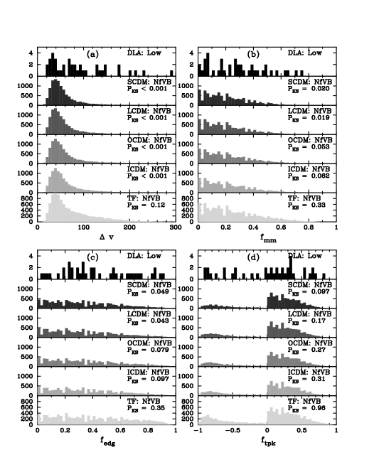
Figure 5: Comparison between empirical and Monte Carlo distributions of low ion test statistics for SCDM, $\Lambda$CDM, OCDM, ICDM, and TF cosmogonies. Results for NfVB model compare distributions of (a) $\Delta v$, (b) $f_{MM}$, (c) $f_{edg}$, and (d) $f_{tpk}$ test statistics which are defined in paper I. Briefly stated these quantities are the (a) absorption velocity interval, (b) the normalized difference between the mean and median velocity, (c) the difference between the velocity of the strongest component and mean velocity, and (d) the difference between the velocity of the second strongest component and mean velocity. The quantity $P_{KS}$ is the KS probability that model and empirical distributions are drawn from the same parent population.

4.2 TF

In the TF cosmogony we either let $N_{\perp}(0)$ equal the empirically determined $N_{0}^{Cor}$ or 10^21.2 cm^-2. As discussed previously $V_{rot}(r)$ = $V_{max}$ in all TF models, where the distribution of $V_{max}$ is shown in Figure 2. Figure 5 also shows the model NfVB results for TF. Here the $\Delta v$ test yields $P_{KS}$($\Delta v$) = 0.12. While lower than $P_{KS}$($\Delta v$) = 0.65 exhibited by models in which every halo has $V_{rot}(r)$ = 250 km s^-1 (PW1), this KS probability is sufficiently large that the more realistic TF model cannot be excluded. We shall check the robustness of these results for the TF and CDM models in $\S$ 6.

5 RESULTS of MONTECARLO SIMULATIONS: IONIZED GAS

5.1 Normalization

In order to fit the simulations to the data it is necessary to specify the function ${\overline{N}_{CIV}(b)}$ where $b$ is the impact parameter. This function is crucial as it constrains kinematic quantities such as $\Delta v_{\rm CIV}$ for the C IV profiles by fixing the number of clouds per line of sight (see eq. 30). We normalize ${\overline{N}_{CIV}(b)}$ by determining the parameters $K$ and $\beta$ (eqs. 28 and 29) from comparisons between model and empirically determined frequency distributions of C IV column densities, $f(N_{CIV},z)$. The latter is the product of the number of damped Ly$\alpha$ systems per unit “absorption distance”, $dn/dX$, times $g(N_{CIV})$, the conditional distribution of C IV column densities given the presence of a damped Ly$\alpha$ system. We find that

$$f(N_{CIV},z)={dn\over dz}{\Biggl{(}}{dX\over dz}{\Biggr{)}}^{-1}g(N_{CIV}),{}$$

$$\ {dX\over dz}={{(1+z)^{2}}\over{[(1+z)^{2}(1+{\Omega_{M}}z)-z(z+2){\Omega_{\Lambda}}]^{1/2}}}\;\;\;.$$ (31)

Because damped Ly$\alpha$ systems are H I selected, the function $g$ will depend on the differential area of the inclined H I disks giving rise to damped Ly$\alpha$ absorption. As a result the $g$ will depend on impact parameter, $b$, and hence on $K$ and $\beta$ through eqs. (28) and (29). We adjust $K$ and $\beta$ by comparing model and empirical $f(N_{CIV},z)$’s.

Figure 6: Comparison between empirical and model CIV column density distributions. The points with error bars are data. The solid and short dashed curves are predictions for MfVB and NfVB models, $\beta$ = 1.5 and the $\Lambda$CDM cosmogony. The short dashed curve corresponds to the MM model for halos with $V_{200}$ $>$ 150 km s^-1 and in which $\beta$ $\approx\ -1$

We constructed the empirical $g(N_{CIV})$ from the 32 C IV column densities inferred from the profiles in Figure 1 in Paper I (The actual column densities are reported in Prochaska & Wolfe 1999 and in Lu et al.  1996). To obtain the empirical $f(N_{CIV},z)$ we adopted the $\Lambda$CDM model and let $dn/dz$ = 0.22 which is appropriate for the mean redshift of this sample. The results are shown as points with error bars in Figure 6. We compare this with the predictions for models MfVB and NfVB in the case of a $\Lambda$CDM cosmology. The results are valid for all MXXX and NXXX models respectively. This is because $f(N_{CIV})$ depends on the distribution of impact parameters, but is independent of rotation speed and infall kinematics. In both classes of models, $\beta$ = 1.5 provides a good fit to the data, while $K$ = 2$\times$10¹⁵ cm^-2 for model MfVB and 2$\times$10¹⁴ cm^-2 for model NfVB. When MM computed ${\overline{N}_{CIV}(b)}$ for cool halo gas photoionized by background radiation, they found K and $\beta$ to vary with $V_{200}$, in contrast to our assumption of uniform $K$ and $\beta$ for halos of all mass. Fortunately, the C IV velocity profiles are independent of $K$ because both ${\overline{N}_{CIV}}$ and $N_{CIV}^{cld}$ are linearly dependent on $K$, and as a result $K$ drops out of the determination of $n_{cld}$ which is crucial in determining the velocity profile widths (see eq. 30). On the other hand the profiles do depend on $\beta$. Figure 6 shows that $\beta$ = $-$ 0.9, which corresponds to the MM results for halos with $V_{200}$ $>$ 150 km s^-1 , results in poor fits to the data. Therefore, the $\beta$ $\approx$ 1.5 assumption is consistent with the C IV data and is used in the calculations which follow.

5.2 Test Statistics

5.2.1 CDM Models

In Figure 7a we compare the empirical $\Delta v_{\rm CIV}$ distribution with predictions by the $\Lambda$CDM cosmogony. We only show results for the case $V_{rot}(r)$=$V_{200}$, since halo kinematics should be unaffected by disk rotation speed for halos of a given mass. We ignore results for the $f_{mm}$, $f_{edg}$, and $f_{tpk}$ statistics because in the case of C IV kinematics $\Delta v_{\rm CIV}$ is the most sensitive test statistic for testing any of the models. The principal difference between the distributions in Figure 7a stems from the different velocity fields at $r$ $\leq$ $r_{cross}$. Models with ballistic infall (MV2B and NV2B) predict larger median $\Delta v_{\rm CIV}$ than models with random motions (MV2R and NV2R). For a given $N_{\perp}(0)$ the ballistic models are in slightly better agreement with the data because the larger $\Delta v_{\rm CIV}$’s are closer to the observed values.

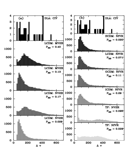
Figure 7: Comparison between empirical and Monte Carlo distribution of $\Delta v_{\rm CIV}$. (a) Results for $\Lambda$CDM cosmogony and MV2B, MV2R, NV2B, and NV2R models. (b) Results for SCDM through ICDM cosmogonies and NfVR model, and for TF cosmogony with NV2R and NfVR models

The value of $N_{\perp}(0)$ also causes differences between the distributions. Comparison between ballistic infall models MV2B and NV2B shows that MV2B predicts lower median $\Delta v_{\rm CIV}$ than NV2B. This is because the higher $N_{\perp}(0)$ of model MV2B results in larger impact parameters then cause the sightlines to sample the halos at larger radii where the infall velocities are smaller. In this case the lower $\Delta v_{\rm CIV}$ of the MV2B model is in better agreement with the data. At the same time model MV2R is in better agreement with the data than NV2R, because the smaller impact parameters predicted by the latter model result in more sightlines traversing the $r$ $\leq$ $r_{cross}$ region where random motions give rise to $\Delta v_{\rm CIV}$ that are also lower.

The third difference between the $\Delta v$ distributions depends on the assumed cosmogony. In Figure 7b we use the NfVR model to illustrate the effects of the assumed cosmology. The cosmogonies differ according to the fraction of halos with large $V_{200}$, a fraction which increases along the SCDM $\rightarrow$ ICDM sequence. In every cosmogony in this Figure a “spike” in the $\Delta v_{\rm CIV}$ distribution at $\Delta v_{\rm CIV}$ = 50 km s^-1 is present and increases in strength along the sequence. The spike arises from sightlines traversing the outer regions of high-mass halos at large impact parameters. The high pressure of hot gas in massive halos (see Figure 3) compresses the clouds thereby reducing their cross-sections. For clouds of fixed mass the result is an increase in column density. In most cases only one cloud is required to satisfy eq. (30) at large $b$ where ${\overline{N}_{CIV}}$ is small. The spike occurs at $\Delta v_{\rm CIV}$ = 50 km s^-1 because this is the FWHM of the profile caused by a single cloud with an assumed internal velocity dispersion, $\sigma_{int}$ = 25 km s^-1 . In fact this value of $\sigma_{int}$ was chosen to reproduce the narrowest C IV profiles in our sample.

It is worth noting that despite their differences most of the models yield large $P_{KS}$($\Delta v_{\rm CIV}$) values. This is in contrast to tests of low ion kinematics. In that case all of the $P_{KS}$($\Delta v_{\rm low}$) values were too small; i.e., none of the models was compatible with the observed distribution of low ion $\Delta v$. This could imply that while the infall interpretation for the high ions is correct, the disk interpretation for the low ions is incorrect.

5.2.2 TF Models

Figure 7 b also compares the data with the predictions of the TF cosmogony. In this case $V_{200}$ equals $V_{max}$ or $V_{max}$/$f_{V}$ where the $V_{max}$ are the input disk rotation speeds. As a result the CDM degeneracy of $\Delta v_{\rm CIV}$ with respect to disk rotation speed is broken in the TF models. We show results for some examples to illustrate this effect. As expected the $\Delta v$ = 50 km s^-1 spike is highest for the NV2R model where $V_{200}$ = $V_{max}$. Because of the larger fraction of halos with high $V_{200}$, the median $\Delta v$’s are higher than in the CDM models. Agreement with the empirical $\Delta v_{\rm CIV}$ distribution improves in the case of random motions at $r\ <r_{cross}$ and when $V_{200}$ = $V_{max}$/$f_{V}$; i.e., with the NfVR model (note the higher P_KS($\Delta v_{\rm CIV}$) value of the NV2R model is an artifact due to the large amplitude spike at $\Delta v_{\rm CIV}$ = 50 km s^-1 ), but the $P_{KS}$($\Delta v_{\rm CIV}$) values are still leass than 0.05.

5.3 Correlation Tests

In Figure 8 we compare empirical and predicted distributions of $\delta v$ and $f_{ratio}$. These are the differences between the mean velocities of the C IV and low ion velocity profiles and the ratio $\Delta v_{\rm CIV}$/$\Delta v_{\rm low}$, respectively . Comparison between empirical and predicted cross-correlation functions for the C IV versus low ion velocity profiles is also shown.

$\bullet$ $\delta v$ Test:

In CDM all the models pass the $\delta v$ test at more than 83$\%$ confidence. In Figure 8a we use $\Lambda$CDM to illustrate the effects of (a) disk rotation speed, (b) impact parameter, and (c) halo velocity field. Comparison between the MfVB and MV2B models shows that disk rotation speed is the most important effect. Specifically $P_{KS}$($\delta v$) increases significantly when $V_{200}$ decreases from $f_{V}$$V_{200}$ to $V_{200}$. This behavior is straightforward to explain. In the disk-halo models the half-width of the $\delta v$ distribution is roughly equal to the sample average of $V_{rot}(r)$sin($i$). This is because the prototypical C IV profile comprises two widely separated absorption components symmetrically displaced about the systemic velocity of the halo. As a result the mean velocity of the C IV profile equals the systemic velocity. On the other hand the low ion profile consists of multiple contiguous components comprising a single feature that is displaced to either side of the systemic velocity. In this case the mean velocity of the low ion profile is separated by $\sim$ $V_{rot}(r)$sin($i$) from the systemic velocity. Consequently the $\approx$ 75 km s^-1 half-width of the observed distribution limits the fraction of rapidly rotating disks. This constraint is especially severe for the TF models where rotation speeds exceeding 200 km s^-1 are typical.

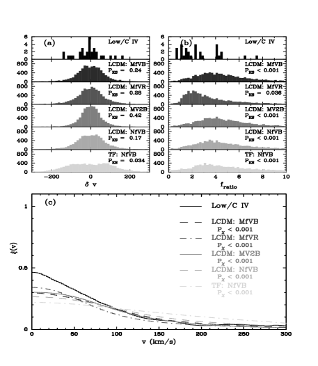
Figure 8: Correlation Tests. (a) Comparison between empirical and Monte Carlo distributions of $\delta v$ for $\Lambda$CDM cosmogony and MfVB, MfVR, MV2B,and NfVB models. The NfVB model is used with the TF cosmogony. (b) Same as (a) but $f_{ratio}$ is substituted for $\delta v$ statistic. (c) Comparison between empirical and Monte Carlo predictions of $\xi(v)$ for C IV versus Low. Same models as in (a) and (b) are used. Curves are data (dark solid curve), $\Lambda$CDM MfVB model (dark dashed curve), $\Lambda$CDM MfVR model (dark dot-dashed curve, $\Lambda$CDM MV2B model (light solid curve), $\Lambda$CDM NfVB model (light dashed curve), and TF NfVB model (light dot-dashed curve)

On the other hand the effects of impact parameter are not as significant. This is because impact parameter affects the width of the velocity features rather than the location of their velocity centroids. This explains why the the MfVB and NfVB results are so similar. Furthermore, the effect of halo velocity field is even less important as shown by comparison between the MfVB and MfVR results. This tells us that for a sufficient number of C IV clouds, the location of the velocity centroid of the C IV profile is independent of whether the clouds are infalling or moving randomly. Therefore, $\delta v$ is set by the magnitude of $V_{rot}(r)$.

$\bullet$ $f_{ratio}$ Test:

A natural consequence of the disk-halo hypothesis is the prediction $f_{ratio}$ $\geq$ 1. Because the infall velocities of the high ions and the rotation speeds of the low ions occur in the same potential well, they both scale linearly with $V_{200}$. However, owing to projection effects, the line-of-sight velocity gradients due to radial infall will exceed those due rotation. Thus, $\Delta v_{\rm CIV}$ will be larger than $\Delta v_{\rm low}$. But the ratios are too large in most CDM models because of the small $\Delta v_{\rm low}$ and the larger $\Delta v_{\rm CIV}$. As a result the best case models are those with large $V_{rot}(r)$ for the disks and random motions at $r$ $\leq$ $r_{cross}$ for the halos. The best model is MfVR, as shown in Figure 8 b. The TF models also produce $f_{ratio}$ that are too high because in most halos the sightlines intercept the region $r\ >r_{cross}$ where large infall velocities are present.

$\bullet$ Cross-Correlation Function:

None of the models, neither CDM nor TF, predicts a cross-correlation function with large enough amplitude to fit the data. The reason is insufficient overlap in velocity space between the C IV and low ion profiles. In Figure 8 c the best case model is MfVR, indicating more overlap occurs when the C IV clouds experience random motions at $r$ $\leq$ $r_{cross}$. Even better agreement is obtained with model MV2R (not shown) implying that overlap increases when the rotation speed of the disk is reduced. This interpretation is supported by the results for the TF models which exhibit the worst agreement with the data. The TF models predict the largest fraction of halos with high $V_{rot}(r)$ and lowest fraction of low-mass halos in which random motions dominate the the velocity field at $r$ $<$ $r_{cross}$.

5.4 Model Summary

In summary we find the following results for the models we haved tested so far:

$\bullet$ While the extent of the low ion $\Delta v$ distribution rules out the single-disk semi-analytic CDM models, it is compatible with the TF models (see also Jedamzik & Prochaska 1998).

$\bullet$ The C IV $\Delta v$ distribution is compatible with most of the CDM models. In the example shown in Figure 7 the best agreement with the data occurs for models with (a) ballistic infall at $r$ $\leq$ $r_{cross}$ and (b) central disk column densities given by $N_{0}^{MMW}$. The best agreement with the TF models is for ballistic infall, $N_{0}$=$N_{0}^{MMW}$, and $V_{200}$ = $V_{max}$/$f_{V}$.

$\bullet$ The $\delta v$ distribution is compatible with all of the CDM models, but is too narrow for the TF models. This is a reflection of the low $V_{rot}(r)$ predicted by CDM and the high $V_{rot}(r)$ predicted by the TF models.

$\bullet$ Most of the CDM models predict $f_{ratio}$ distributions with median values that are too large. This stems from the low values predicted for $V_{rot}(r)$. The same problem holds for the TF models, but in this case the high $f_{ratio}$ stems from the high values of $\Delta v_{\rm CIV}$. In both cosmogonies some models cannot be ruled out.

$\bullet$ None of the models predicts C IV versus low ion cross-correlation functions in agreement with the data.

6 PARAMETER TESTS

The results of the last section may be summarized as follows: When the free parameters of a given model are adjusted to satisfy one test, the model inevitably fails a different test. If this is a generic feature of the disk-halo models, then they may not apply to the damped Ly$\alpha$ systems. This is an important conclusion and we wish to determine how robust it actually is. Indeed the models are characterized by several free parameters that are not well determined, and it is possible we have not found the optimal set. For this reason we now investigate the sensitivity of our conclusions to variations of these parameters.

In a series of trial runs we found the model kinematics to be most sensitive to three parameters. The first is the central perpendicular column density, $N_{\perp}(0)$. Because the range of impact parameters is limited by $N_{\perp}(0)$, it influences both $\Delta v_{\rm CIV}$ and $\Delta v_{\rm low}$. To test the dependence of the kinematics on this quantity we simulate H I disks with $N_{\perp}(0)$ ranging between 10^20.8 and 10^22.2 cm^-2. These values cover the low column densities of the $NXXX$ models and approach the high values of the $MXXX$ models. The second parameter is $V_{cut}$, the low-end cutoff to the distribution of input $V_{200}$ in the CDM models or of input $V_{max}$ in the TF models. The kinematic results should be sensitive to $V_{cut}$ especially in the case of CDM where $V_{cut}$ is at the peak of the $V_{200}$ distribution (see Figure  2). The value used in our models, $V_{cut}$ = 30 km s^-1 , is imposed by thermal expansion of photoionized gas out of the potential wells of halos with $V_{200}$ lower than this (Thoul & Weinberg 1995). However feedback due to supernova explosions might drive gas out of disks with $V_{200}$ as large as 100 km s^-1 (see Dekel & Silk 1986, but see MacLow & Ferrara 1999). For these reasons we let $V_{cut}$ vary between 30 and 120 km s^-1 . The third parameter is the C IV column density per cloud, $N^{cld}_{CIV}$. The definition given in eqs. (25)$-$(27) is for a spherical cloud of a given mass and C⁺³/H ratio, i.e., $X_{CIV}$. To account for deviations from spherical symmetry or from our definition of $X_{CIV}$ (see eq. 26) we introduce the parameter $q_{CIV}$ which is the ratio of the true C IV column density to our model definition. We let $q_{CIV}$ vary between 0.1 and 1.3. In order to supply the total C IV column density required at a given impact parameter, the number of clouds must increase as $q_{CIV}$ decreases. This affects the C IV kinematics because $\Delta v_{\rm CIV}$ will increase with cloud number.

6.1 CDM

The results of the parameter tests are summarized in Figure  9 which shows iso-probability contours in the $V_{cut}$ versus $N_{\perp}(0)$ plane. The contours correspond to 0.01, 0.05, and 0.32 for $P_{KS}$($\Delta v$_low) (9a), $P_{KS}$($\Delta v$_CIV) (9b), $P_{KS}$($\delta v$) (9c), and $P_{KS}$($f_{ratio}$) (9d). We show results for $q_{CIV}$ = 1.0 since smaller values are found to result in $f_{ratio}$ that are too large. We choose a variant of the NfVR model in which $N_{\perp}(0)$ is a free parameter. We abandon ballistic infall in favor of random motions at $r$ $<$ $r_{cross}$ because we find that random motions produce more overlap in velocity space between low ion and C IV profiles and as a result they produce better agreement between model predictions and the empirical test statistics.

Figure 9: Iso-probability contours in $V_{cut}$ versus $N_{\perp}(0)$ plane resulting from parameter search of $\Lambda$CDM cosmogony where NfVR model is assumed in which is a free parameter and where $q_{CIV}$ = 1.0. Contours correspond to $P_{KS}$ = 0.32 (solid lines), 0.05 (dots), and 0.01 (dashes). Tests are (a) $\Delta v_{\rm low}$, (b) $\Delta v_{\rm CIV}$, (c) $\delta v$, and (d) $f_{ratio}$.

Figure  9a shows the results for the low ion $\Delta v$ test. As expected models with the standard value $V_{cut}$ = 30 km s^-1 are improbable for reasonable values of $N_{\perp}(0)$. Rather $V_{cut}$ increases along the $P_{KS}$($\Delta v_{\rm low}$) = 0.05 contour from 35 km s^-1 at $\log N_{\perp}(0)=20.8$ cm^-2 to 105 km s^-1 at $\log N_{\perp}(0)=22.0$ cm^-2. An increase in $N_{\perp}(0)$ means larger impact parameters which in turn imply smaller $\Delta v_{\rm low}$ (see $\S$ 5.1). Therefore, an increase in $V_{cut}$ must accompany the increase in $N_{\perp}(0)$ to boost the fraction of high-$V_{200}$ halos required to maintain the extent of the $\Delta v_{\rm low}$ distribution. By contrast Figure  9b shows that $V_{cut}$ hardly varies with $N_{\perp}(0)$ along the $P_{KS}$($\Delta v$_CIV) contours. In our CDM models most sightlines traverse halos with low $V_{200}$ where cloud motions in NfVR models are dominated by random velocities drawn from a Gaussian with dispersion that is an insensitive function of radius (eq. D4). Consequently $\Delta v_{\rm CIV}$ will be independent of impact parameter and hence independent of $N_{\perp}(0)$. Therefore, $V_{cut}$ need not vary with $N_{\perp}(0)$ to maintain the extent of the $\Delta v_{\rm CIV}$ distribution.

Figure  9c and d shows the iso-probability contours for the $\delta v$ and $f_{ratio}$ tests. In Figure  9c none of the contours rises to $P_{KS}$($\delta v$) = 0.32 in the $V_{cut}$ versus $N_{\perp}(0)$ plane. The shape of the $P_{KS}$($\delta v$) = 0.05 contour has the following implications. First, the insensitivity of the contour to $N_{\perp}(0)$ just indicates that the displacement of the low ion velocity centroid from the systemic velocity of the galaxy is determined by rotation speed rather than $\Delta v_{\rm low}$. Second, models with $V_{cut}$ $>$ 55 km s^-1 are highly unlikely as they produce $\delta v$ that are too large. In Figure  9d, $N_{\perp}(0)$ decreases with increasing $V_{cut}$ along all iso-probability contours. Because $\Delta v_{\rm CIV}$ increases with increasing $V_{cut}$, $N_{\perp}(0)$ must show a corresponding decrease to boost $\Delta v_{\rm low}$. Otherwise $f_{ratio}$ becomes larger than observed.

Figure  10 shows the $P_{KS}$ = 0.05 contours from the previous Figure. The horizontal lines trace out the region in the $V_{cut}$ versus $N_{\perp}(0)$ plane in which $P_{KS}$ $\geq$ 0.05 for all 4 tests; i.e., the parameter space of acceptable models. Physically, the resulting range of $V_{cut}$ (i.e. 35 to 50 km s^-1 ) is acceptable for models in which gas photoionized by ionizing background radiation escapes from low-mass halos (Thoul & Weinberg 1995; Navarro & Steinmetz 1997). On the other hand the upper limit on $N_{\perp}(0)$ (i.e., $\log N_{\perp}(0)<21.2$ cm^-2) may be too low to explain the shape of the H I column-density distribution function (see $\S$ 7). Furthermore, this Figure indicates these models may not be viable as they occupy a small fraction of the depicted parameter space. Notice that the horizontal $\delta v$ contour at $V_{cut}$ $\approx$ 50 km s^-1 is crucial in restricting the acceptable region to such a small area. Because $\delta v$ is set by rotation speed we investigated the NV2R models to determine whether the lower rotation speeds would enlarge the acceptable region. The results are shown in Figure  11. As predicted the lower rotation speeds lift the restricting $\delta v$ contour from $\approx$ 50 to $\approx$ 95 km s^-1 . However, the lower rotation speeds also increase $f_{ratio}$, with a consequent lowering of the $P_{KS}(f_{ratio})$ contour in Figure  11d. Consequently there is no region in the $V_{cut}$ verus $N_{\perp}(0)$ plane in which all 4 tests result in $P_{KS}$ $\geq$ 0.05 for the NV2R model. Therefore, our conclusion concerning the size of acceptable regions in parameter space appears to be robust.

Figure 10: solid lines are contours corresponding to $P_{KS}$ = 0.05 in Figure 9. The region in which $P_{KS}$ $\geq$ 0.095 for all 4 tests is denoted by horizontal lines

Figure 11: Same as Figure 9, except with NV2R model

Turning to the cross-correlation function we find that none of the models within the range of $V_{cut}$ and $N_{\perp}(0)$ depicted in Figure  9 results in C IV versus low ion cross-correlation functions with acceptable $\chi^{2}$ values. Apparently the combination of radial infall and disk rotation produce C IV and low ion absorption profiles with insufficient overlap in velocity space to explain the data. Better agreement is obtained when $\log N_{\perp}(0)>23$ cm^-2. But column densities this high are ruled out by the other tests. We shall return to this dilemma in $\S$ 7.

In summary, by varying $V_{cut}$, $N_{\perp}(0)$, and $q_{CIV}$ we find regions of parameter space where the $\Lambda$CDM models are in better agreement with the data than for the “standard” values of the parameters adopted above. This is especially true for the low ion $\Delta v$ test which ruled out most of the “standard” models (where $V_{cut}$ = 30 km s^-1 ). However, the models may still not be viable because of the restricted range of allowable parameters, and because none of the models is compatible with the C IV versus low ion cross-correlation function.

6.2 TF

The corresponding results for the TF models are shown in Figure  12. In this case the best fit value of $q_{CIV}$ equals 1.3. Figure  12a illustrates the results for the low ion $\Delta v$ test. The Figure shows the $P_{KS}$($\Delta v$_low) = 0.05 contour to enclose a larger area of parameter space than in the CDM case. As in CDM, $V_{cut}$ increases with $N_{\perp}(0)$ along iso-probability contours. However, the $\Delta v_{\rm low}$ contours are less sensitive to $V_{cut}$ because the input halo distribution does not peak at $V_{cut}$ as in CDM (see Figure 2). Figure  12b shows that by contrast with CDM the $P_{KS}$($\Delta v$_CIV) contours are sensitive functions of $N_{\perp}(0)$. This is because in the TF model more sightlines traverse high $V_{200}$ halos where C IV clouds undergo infall at $r$ $>$ $r_{cross}$, and as a result $\Delta v_{\rm CIV}$ is a sensitive function of impact parameter, and therefore of $N_{\perp}(0)$.

Figure 12: Same as Figure 11, but for TF cosmogony

The results for the $\delta v$ and $f_{ratio}$ tests are plotted in Figure  12c and d. All of the models result in $P_{KS}$($\delta v$) $<$ 0.05. Clearly the large fraction of rapidly rotating disks encountered in the TF model produces $\delta v$ that are too high. By contrast the results for the $f_{ratio}$ lead to $P_{KS}$($\delta v$) $>$ 0.05 throughout the parameter space depicted in the Figure except for the upper right portion where $P_{KS}$($\delta v$) $>$ 0.32. But part of the improvement here is caused by spikes in the $\Delta v_{\rm CIV}$ distribution near 50 km s^-1 which prevent $f_{ratio}$ from exceeding observed values when the $\Delta v_{\rm low}$ are small. While the physical basis for such spikes is understood (see $\S$ 5.2.1), they have not been confirmed by the data. As in CDM, none of the TF models produce C IV versus low ion cross-correlation functions with acceptable $\chi^{2}$ values. In fact the higher fraction of disks with large rotation speeds predicted by the TF model increases the displacement between low ion and C IV profiles which produces even lower cross-correlation amplitudes than in the CDM models.

We also tested the sensitivity of the TF model results to variations of (a) $\gamma$ and $V_{*}$, the power-law exponent and fiducial rotation speed in the Tully-Fisher relation (see eq. 13), and (b) the Schecter function exponent, $\alpha$ (see eq. 15). Within the parameter range, 3 $<$ $\gamma$ $<$ 4, (cf. Giovanelli et al.  1997; Sakai et al.  2000) the test statistic distributions do not change significantly. By contrast, increasing $\alpha$ above 1.2 reduces $\Delta v_{\rm low}$ significantly owing to the larger fraction of low mass halos. This would occur if the damped Ly$\alpha$ galaxies were drawn from the luminosity function measured for the Lyman-break galaxies (Steidel et al.  1999), since in that case $\alpha$ = 1.6 (see $\S$ 2.1). But overall the improvement of the model is poor because $f_{ratio}$ increases to unacceptably high values. The results also change when we vary $V_{*}$ above 280 km s^-1 or below 220 km s^-1 . But in both cases the model does better against some tests and worse against others. In no case did the TF model pass all 4 tests at more than 95 $\%$ nor did the fits of the cross-correlation function become acceptable. In that sense the TF models are in worse agreement with the data than the CDM models.

7 SUMMARY AND CONCLUDING REMARKS

We used accurate kinematic data acquired for a sample of 35 damped Ly$\alpha$ systems to test the standard paradigm of galaxy formation; i.e., the scenario in which galaxies evolve from the dissipative collapse of virialized gaseous halos onto rotating disks. The data was presented in the form of velocity profiles of high ions, intermediate ions, and low ions in Paper I. In this paper we considered semi-analytic models, specifically the MMW models in which centrifugally supported exponential disks are located at the centers of dark matter halos drawn from mass distributions predicted by standard CDM cosmogonies, and where infall of ionized gas from the halo occurs. We also considered the null hypothesis that current disk galaxies were in place at $z$ $>$ 3 (the TF models). We tested the models with Monte Carlo techniques by comparing distributions of test statistics generated from observed and model velocity profiles. We utilized eight test statistics: $\Delta v_{\rm low}$, $f_{edg}$, $f_{mm}$, and $f_{tpk}$ for the low ion profiles (see Paper I), $\Delta v_{\rm CIV}$ for the C IV profiles, and $\delta v$, $f_{ratio}$, and $\xi(v)$ for comparing low ion and C IV profiles.

First, we discuss the general implications of our work. As discussed in Paper I velocity profiles overlapping in velocity space in such a way that $\Delta v_{\rm CIV}$ $\geq$ $\Delta v_{\rm low}$ are naturally reproduced by scenarios where low ion and high ion kinematic subsystems are in the same gravitational potential well. In the collapse scenario the velocity fields of both subsystems scale as $V_{200}$, yet more of $V_{200}$ is projected along the line of sight by gas undergoing radial infall than by gas confined to rotating disks. This was confirmed by our Monte Carlo simulations of radial infall of ionized gas clouds onto neutral rotating disks. Indeed in some cases the infall velocities exceed $V_{200}$ resulting in $\Delta v_{\rm CIV}$/$\Delta v_{\rm low}$ ratios that are too large. By contrast, scenarios in which the high ions are embedded in gaseous outflows (e.g. Nulsen et al.  1998) or any flows not generated by dark-matter potentials determining low ion velocities will in general not satisfy these constraints.

Next we discuss specific conclusions arising from this work, in particular the results of model testing. Tests of models with the standard parameters discussed in $\S$ 4 and $\S$ 5 led to the following conclusions:

(1) In the case of the low ion gas none of measured distributions of $\Delta v_{\rm low}$, $f_{edg}$, $f_{mm}$, and $f_{tpk}$ were compatible with the predictions of the CDM cosmogonies at the 95$\%$ confidence level. By comparison, the TF model was compatible with the data at 88 $\%$ confidence level.

(2) For the high ion gas we considered only the $\Delta v_{\rm CIV}$ distribution. Comparison with the data showed CDM models with the high column densities predicted by MMW, i.e., $N_{\perp}(0)=N_{\perp}(0)^{MMW}$, were in good agreement with the data. CDM models with significantly lower $N_{\perp}(0)$ were not as good because they produced overly large $\Delta v_{\rm CIV}$. For the same reasons TF models with high $N_{\perp}(0)$ were in better agreement with the data than with low $N_{\perp}(0)$.

(3) To test model predictions for the relative properties of the high ion and low ion gas we considered the $\delta v$ distribution. The CDM models were compatible with the data while TF models were not. Apparently the high rotation-speed TF disks displace the asymmetric low ion profiles too far from the velocity centroids of the C IV profiles.

(4) Tests of the $f_{ratio}$ distributions showed neither CDM nor TF model predictions agreed with the data at 95 $\%$ confidence.

(5) Neither the CDM nor TF models predicted C IV versus low ion cross-correlation functions that were compatible with the data at 99 $\%$ confidence.

We then explored parameter space to determine whether these conclusions were robust (see $\S$ 6). We varied three crucial parameters: $V_{cut}$, $N_{\perp}(0)$, and $q_{CIV}$. This exercise led to the following conclusions:

(6) Figure 9 shows that the NfVR-$\Lambda$CDM model is compatible with the $\Delta v_{\rm low}$, $\Delta v_{\rm CIV}$, $\delta v$, and $f_{ratio}$ tests at more than 95 $\%$ confidence throughout the small area of the $V_{cut}$ versus $N_{\perp}(0)$ plane shown in Figure 10. This is a serious shortcoming since the NfVR model used for the comparison is “optimistic” in that it predicts a constant velocity rotation curve with maximum rotation speed $V_{rot}(r)$ = $f_{V}$$V_{200}$. It also predicts low impact parameters owing to the restriction $N_{\perp}(0)\ <10^{21.2}$ cm^-2. In addition, a small decrease in disk thickness would eliminate consistency throughout parameter space; i.e., the disks must be thick.

(7) Figure 12 shows the NfVR-TF model to be compatible with the $\Delta v_{\rm low}$, $\Delta v_{\rm CIV}$, and $f_{ratio}$ tests and incompatible with the $\delta v$ test at the 95 $\%$ confidence.

(8) Neither CDM nor TF models produce C IV versus low ion cross correlation functions that were consistent with the data in the parameter space shown in these Figures.

What have we learned from the model tests? Because the CDM models pass 4 out of 5 tests and the TF models pass 3 out of 5 tests, the CDM models appear to be more plausible. But to achieve this result it was necessary to adopt a flat rotation curve with $V_{rot}(r)$ = $f_{V}$$V_{200}$. This is the maximum rotation speed possible for a model disk, and $V_{rot}(r)$ in realistic protogalactic disks are probably lower. However, Figure 11 shows that a parameter search for models with $V_{rot}(r)$=$V_{200}$ reveals no region in parameter space which is compatible with the 4 kinematic tests at 95 $\%$ confidence. Second, the limit $N_{\perp}(0)<10^{21.2}$ cm^-2 indicates that exponential disk models should predict a steepening of the column-density distribution function at $N$ $>$ 10^21.2 cm^-2. This effect is not present in the data (Wolfe et al.  1995; Rao & Turnshek 1999). Third, the failure of any model to reproduce the C IV versus low ion $\xi(v)$ indicates significant overlap in velocity space between the low ion and high ion velocity fields was not achieved. Fourth, the CDM models predict that most of the damped Ly$\alpha$ systems occur in low mass halos where the kinematic state of the ionized gas is highly uncertain (see $\S$ 3.1).

Does this mean that disk-halo models for damped Ly$\alpha$ systems are ruled out? We think it is premature to reach this conclusion. Rather we take these results to mean that if the collapse scenario is correct, a stronger coupling between the kinematic subsystems is required. One possibility that comes to mind is for low ions to be associated with the infalling C IV clouds. This would increase the low ion line-of-sight velocities and cause smaller differences between the C IV and low ion velocity profiles. But the problem is there is no evidence for low ions with high ion kinematics. Another way to couple the subsystems is to include the angular momentum of the halo gas. This is neglected in the radial infall model. As the C IV clouds approach the disk they spin up and experience azimuthal velocity components approaching $V_{rot}(r)$. The idea is plausible if the angular momentum vector of the infalling gas is related to that of the disk, and if clouds near the disk are likely to be detected. It is encouraging that recent N-body simulations show the angular momenta of disk and halo to be correlated (Weinberg 2000). It is also encouraging that the density of clouds along the line of sight is highest near the disk. Still, if this idea doesn’t work one would be forced to abandon the disk-halo hypothesis; i.e., one of the standard paradigms of galaxy formation.

Can the kinematic data be better explained by scenarios other than infall of ionized gas onto rotating disks of neutral gas? First, we already discussed problems associated with outflow models. Second, lacking analytic expressions for the various quantities, it is not clear whether numerical simulations of damped Ly$\alpha$ systems are compatible with the kinematics of the ionized gas. However, the density contours in Haehnelt et al. (1998) show the C IV clouds to be within $\sim$ 10 kpc of the low ion clouds in which case both would be subjected to the same dark-matter gravitational field. Because the low ion gas is not confined to rotating disks, it is not obvious why the predicted $f_{ratio}$ should exceed the observed lower limit of unity. To satisfy this constraint one must consider contributions to the C IV profiles from gas outside the dark-matter halos, perhaps in the fashion described by Rauch et al. (1997) for the C IV QSO absorption lines. Third, the scenario described by the semi-analytic modeling of Maller et al.  (2000) may provide a good fit to the C IV kinematics. In particular, both the low ion and C IV kinematics arise from the orbital motions of mini-halos accreted onto more massive halos with $V_{200}$ $\sim$ 150 km s^-1 , implying $\Delta v_{\rm CIV}$ $\geq$ $\Delta v_{\rm low}$ and that C IV and low ion profiles are well correlated. The current difficulty with the model is to physically motivate the very large Mestel disks required to explain the low ion kinematics. In any case performing the tests outlined in this paper will reveal how robust these models actually are.

Appendix A Press-Schecter Theory for ICDM Cosmogonies

According to Press-Schecter theory the density of bound halos is in the mass interval $(M,M+dM)$ is given by

$$n(M,z)dM=-2{\rho\over M}{{\partial F}\over{\partial M}}dM\;\;\;,$$ (A1)

where $\rho$ is the mean density of matter and $F$ is the fraction of objects with masses $\leq$ M that collapsed by redshift, $z$. For Gaussian distributed density fields, $F$ is given by

$$F=(1/2)\Bigg{[}1-{\rm erf}\bigg{(}{\delta_{c}\over{\sqrt{2}}D(z){\Delta_{0}(M)}}\bigg{)}\Bigg{]}\;\;\;,$$ (A2)

where $D(z)$ is the density-contrast growth factor (Peebles 1980) and $\Delta_{0}(M)$ is the current rms density contrast with mass $M$. While eq. (A2) is applicable to ACDM models, it does not apply to ICDM models where the density contrasts are not Gaussian distributed. Rather, we shall use an analytic fit to results of numerical computations (Peebles 1998b) which shows that in ICDM, $F$ is given by

$$F=0.37{\rm exp}{\bigg{[}}-0.67{\bigg{(}}{{\delta_{c}}\over D(z){\Delta_{0}(M)}}\bigg{)}\bigg{]}\;\;\;.$$ (A3)

For power spectra in which $P(k)$ $\propto$ $k^{n}$, $\Delta_{0}(M)$ $\propto$ $M^{-({{n+3}\over 6})}$. As a result

$${\rm ICDM}:n(M,z)dM=0.5{\rho\over M}\bigg{(}{M\over M_{*}}\bigg{)}^{({{n+3}\over 6})}$$

$$\times\;{\rm exp}\Bigg{[}-0.67\bigg{(}{M\over M_{*}}\bigg{)}^{({{n+3}\over 6})}\Bigg{]}\bigg{(}{n+3\over 6}\bigg{)}{dM\over M}\;\;\;,$$ (A4)

where $M_{*}$, the mass going non-linear at redshift $z$, is obtained from the expression, $\Delta_{0}(M_{*})$ = $\delta_{c}/D(z)$ (see White 1997). One finds that

$$M_{*}(z)=M_{8}{\bigg{[}}{{\Delta_{0}(M_{8})}\over{\delta_{c}}}{\bigg{]}}^{{6}\over{n+3}}{\bigg{[}}D(z){\bigg{]}}^{{6}\over{n+3}}\;\;\;,$$ (A5)

where the mass in a sphere with radius $R$ = 8$h^{-1}$ Mpc, $M_{8}$ = 5.9$\times$ 10¹⁴$\Omega_{M}$$M_{\odot}$. Throughout the paper, we denote $\Delta_{0}(M_{8})$ by the more conventional symbol, $\sigma_{8}$. In the case of Gaussian linear density fields applicable to ACDM models we have

$${\rm ACDM}:n(M,z)dM=-{\sqrt{2\over\pi}}{\rho\over M}{{\delta_{c}}\over D{\Delta_{0}}^{2}}{d\Delta_{0}\over dM}$$

$$\times\;{\rm exp}{\Bigg{[}}-{{\delta_{c}^{2}}\over 2D^{2}{\Delta_{0}^{2}}}{\Bigg{]}}dM\;\;\;,$$ (A6)

where in this case $\Delta_{0}(M)$ is determined by the full CDM power spectrum (Bardeen et al.  1986).

Appendix B Hot Gas in NFW Halos

Following MM we assume the hot gas is in hydrostatic equilibrium with the dark matter potential and exhibits adiabatic temperature and density profiles out to $r_{min}$ = min($r_{cool}$,$r_{200}$). For the NFW rotation curves given in eq. (7) the density and temperature profiles of hot gas within $r_{min}$ are given by

$$\rho_{h}(r) =\rho_{h}(r_{min})[1+0.8Z_{NFW}(r)]^{3/2}\;\;\;;$$

$$T_{h}(r) =T_{h}(r_{min})[1+0.8Z_{NFW}(r)]\;\;\;;$$

$$0<r<r_{min}\;\;\;,$$ (B1)

where

$$Z_{NFW}(r)={c\over{\delta_{NFW}}}{\Biggl{[}}{{{\rm ln}(1+x)}\over x}-{{{\rm ln}(1+x_{min})}\over x_{min}}{\Biggr{]}}\;\;\;;x=r/r_{s}\;\;\;,$$ (B2)

and

$${\delta_{NFW}}=[{\rm ln}(1+c)-c/(1+c)]\;\;\;.$$ (B3)

At $r\ >r_{min}$ the hot gas either follows isothermal profiles when $r_{200}$ $>$ $r_{cool}$ or does not exist when $r_{200}$ $<$ $r_{cool}$. The temperature and density of hot gas at $r_{min}$ are given by

$$\ T_{h}(r_{min})=T_{vir}\;\;\;,$$ (B4)

and

$${\rho_{h}(r_{min})}={f_{g}V^{2}_{200}\over 4{\pi}Gr^{2}_{s}}{c\over{\delta_{NFW}}}{1\over{x_{cool}(1+x_{cool})^{2}}}\;\;\;;x_{cool}=r_{cool}/r_{s}\;\;\;.$$ (B5)

where $f_{g}$ is the mass fraction in gas. To solve for $r_{cool}$ we follow MM and let ${\rho_{h}(r_{min})}$ = 5$({\mu}m_{H})^{2}$$V_{200}$²/4$\Lambda(T_{vir})t_{M}$ where ${\Lambda(T)}$ is the cooling function. From the last equation we find that $x_{cool}$ is the root of the following polynomial:

$$x_{cool}(1+x_{cool})^{2}-(c/{\delta_{NFW}})(R_{cool}/r_{s})^{2}=0\;\;\;,$$ (B6)

where $R_{cool}$, the cooling radius of a singular isothermal sphere, is given by

$$R_{cool}={\Biggl{(}}{\Lambda(T_{v})t_{M}m_{d}\over 5{\pi}G{\mu}^{2}m_{H}^{2}}{\Biggr{)}^{1/2}}\;\;\;,$$ (B7)

(see MM). The root of interest is given by $x_{cool}\ \geq$ 1.

Appendix C Cool Gas

The cool gas in the halo comprises photoionized clouds formed from hot phase gas at $r$ $\leq$ $r_{min}$ where $r_{min}$ = min($r_{cool}$,$r_{200}$). Therefore, the mass of gas in the cool phase is given by

$$M_{cool}=f_{g}M(r_{min})-M_{h}(r_{min})\;\;\;,$$ (C1)

where $M(r_{min})$, the total mass within $r_{min}$, and $M_{h}(r_{min})$, the mass of hot gas within $r_{min}$, are given by

$$M(r_{min})={{r_{min}V^{2}_{rot}(r_{min})}\over G}\;\;\;,$$ (C2)

and

$$M_{h}(r_{min})={\int_{0}^{r_{min}}4{\pi}r^{2}{\rho_{h}(r)}dr}\;\;\;.$$ (C3)

For NFW halos we use the rotation curve in eq. (7) to relate $V_{rot}(r_{min})$ to $V_{200}$, eqs. B1$-$B4 to compute the integral in eq. C3, and finally eq. B5 to evaluate $\rho_{h}(r_{min})$. The result is

$$M_{cool}={{f_{g}r_{200}V^{2}_{200}}\over G{\delta_{NFW}}}{\Biggl{[}}{\rm ln}(1+x_{min})-{x_{min}\over(1+x_{min})}$$

$$-{{I_{NFW}(x_{min})}\over{(x_{cool})(1+x_{cool})^{2}}}\Biggr{]}\;\;\;;x=r/r_{s}\;\;\;,$$ (C4)

where

$$I_{NFW}(x_{min})={\int_{0}^{x_{min}}x^{2}[1+0.8Z_{NFW}(x)]dx}\;\;\;.$$ (C5)

MM assume the following form for the density of the cool gas:

$$\rho_{c}(r)={M_{cool}\over{4{\pi}r^{2}V_{c}t_{M}}}\;\;\;,$$ (C6)

where $V_{c}$ is a characteristic infall velocity. Combining the last equation with $\rho_{c}(r)$ = $C_{1}/r^{2}$, we have

$$C_{1}={f_{g}r_{200}V^{2}_{200}\over 4\pi GV_{c}t_{M}\delta_{NFW}}\Biggl{[}\ln(1+x_{min})-{x_{min}\over(1+x_{min})}$$

$$-{I_{NFW}(x_{min})\over(x_{cool})(1+x_{cool})^{2}}\Biggr{]}\;\;\;.$$ (C7)

Having obtained $C_{1}$ we compute $r_{cross}$ by combining these results with eq. (17). We find $r_{cross}$ to be the roots of the following equation:

$$r^{2}[1+Z_{NFW}(r)]^{5/2}-{{C_{1}T_{c}}\over{{\rho_{h}(r_{min})}{T_{h}(r_{min})}}}=0\;\;\;.$$ (C8)

We compute the cloud cross-section, $A(r)$, by combining these results with eq. 18. We find that

$$A(r)={\pi}\left\{\begin{array}[]{ll}{C_{2}}M^{2/3}_{cld}(r)[1+Z_{NFW}(r)]^{-5/3}\ ;r>r_{cross}\\ {C_{3}}M^{2/3}_{cld}(r_{cross}){(r/r_{min})^{4/3}}\ ;r<r_{cross}\;\;\;,\end{array}\right.$$ (C9)

where

$$C_{2}={\Biggl{[}}{3T_{c}\over 4{\pi}{\rho_{h}(r_{min})}T_{h}(r_{min})}{\Biggr{]}^{2/3}},C_{3}={\Biggl{[}}{3r_{min}^{2}\over 4{\pi}C_{1}}{\Biggr{]}^{2/3}}\;\;\;.$$ (C10)

We compute the cloud mass by integrating eq. (19) from $r_{min}$ to $r$ to find $M_{cld}(r)$ at $r\ >r_{cross}$, and assume $M_{cld}(r)=M_{cld}(r_{cross})$ at $r\ <r_{cross}$. We find that

$$M_{cld}(r)=\left\{\begin{array}[]{ll}M_{cld}(r_{min}){\Biggl{[}}1+{{\pi}{\rho_{h}(r_{min})}C_{2}r_{s}\over 3M^{1/3}_{cld}(r_{min})}{\int_{r/r_{s}}^{r_{min}/r_{s}}[1+0.8Z_{NFW}(x)]^{-1/6}}dx{\Biggr{]}^{3}}\ ;r>r_{cross}\\ M_{cld}(r_{cross})\ ;r<r_{cross}\;\;\;.\end{array}\right.$$ (C11)

Appendix D Cloud Kinematics

The infall velocities of the clouds are computed as follows. At $r\ >r_{cross}$ we compute $V_{r}(r)$ from eq. (22) by using the solutions for $M_{cld}(r)$ given in Appendix C and noting that the gravitational acceleration is given by $g(r)$ = ${V^{2}_{rot}(r)}/r$. From eq. (7) we find

$$g(r)={V^{2}_{200}}{1\over r_{s}}{c\over{\delta_{NFW}}}{1\over x^{2}}\Bigl{[}{\rm ln}(1+x)-{x\over 1+x}\Bigr{]}\ ;x=r/r_{s}\ \;\;\;.$$ (D1)

At $r\ <r_{cross}$ we consider two scenarios. In the case of ballistic infall we assume $M_{cld}(r)$ = const. For clouds with infall velocity $V_{r}(r_{cross})$ at $r=\ r_{cross}$, the ballistic solution for NFW halos is given by

$$V^{bal}_{r}(x)=\Biggl{[}V^{2}_{r}(r_{cross})+V^{2}_{200}{2c\over\delta_{NFW}}\biggl{[}{\ln(1+x)\over x}-$$

$${\ln(1+x_{cross})\over x_{cross}}\biggr{]}\Biggr{]}^{1\over 2}\;\;\;;\quad x=r/r_{s}\;\;\;.$$ (D2)

In the case where the kinematics are dominated by random motions we solve the Jeans equations for $\sigma_{r}(r)$, the radial velocity dispersion of the clouds, assuming locally isotropic velocity dispersions (Binney & Tremaine 1987). In this case we have

$${\sigma_{r}(r)^{2}}={1\over{\nu(r)}}{\int_{r}^{\infty}}dx{\nu(x)}g(x)\;\;\;,$$ (D3)

where ${\nu(r)}$ is the average density of clouds. Assuming $\nu(r)$ $\propto$ $\rho_{c}(r)$ we find that

$${\sigma_{r}^{2}(r)}={V^{2}_{200}}{\Biggl{(}}{c\over 3{\delta_{NFW}}}{\Biggr{)}}{\Biggl{[}}{\Biggl{(}}{1\over x}-2x^{2}{\Biggr{)}}{\rm ln}(1+x)+$$

$$2x^{2}{\rm ln}(x)+2x-1{\Biggr{]}}\ ;x=r/r_{s}\ \;\;\;.$$ (D4)

References

- Bardeen et al. (1986) Bardeen, J. M., Bond, J. R., Kaiser, N., & Szalay, A. S. 1986, ApJ, 304, 15
- Baugh et al. (1998) Baugh, C. M., Cole, S., Frenk, C. S., & Lacey, C. G. 1998, ApJ, 498, 504
- Benjamin & Danly (1997) Benjamin, R. A., & Danly, L. 1997, ApJ, 481 764
- Binney & Tremaine (1987) Binney, J., & Tremaine, S. 1987, Galactic Dynamics, (Princeton: University Press), p. 198
- Blumenthal et al. (1986) Blumenthal, G. R., Faber, S. M., Flores, R., & Primack, J. R. 1986, ApJ, 301, 27
- Courteau (1996) Courteau, S. 1996, ApJS, 103, 363
- Courteau (1997) Courteau, S. 1997, AJ, 114 2402
- Dekel & Silk (1986) Dekel, A., & Sily, J. 1986, ApJ, 303 39
- Fabian (1994) Fabian, A. 1994, ARA&A, 32 277
- Giovanelli et al. (1997) Giovanelli, R., Haynes, M. P., da Costa, L. N., Freudling, W., Salzer, J. J., & Wegner, G. ApJ, 477, L1
- Gonzalez et al. (2000) Gonzalez, A. H., Williams, K. A., Bullock, J. S., Kolatt, T. S., & Primack, J. R. 2000, ApJ, 528, 145
- Haehnelt et al. (1998) Haehnelt, M. G., Steinmetz, M., & Rauch, M. 1998 ApJ, 495 647
- Jedamzik & Prochaska (1998) Jedamzik, K., & Prochaska, J. X. 1998 MNRAS, 296 430
- Kauffmann (1996) Kauffmann, G. 1996, MNRAS, 281, 475
- Kepner et al. (1997) Kepner, J. V., Babul, A., Spergel, D. N. 1997, ApJ, 487, 61
- Lin & Murray (2000) Lin, D. N. C., & Murray 2000, astro-ph 0004055
- Loveday et al. (1999) Loveday, J., Tresse, L., & Maddox S., MNRAS, 1999, 310, 281
- Lu et al. (1996b) Lu, L., Sargent, W.L.W., Barlow, T.A., Churchill, C.W., & Vogt, S. 1996, ApJS, 105, 475
- McDonald & Miralda (1999) McDonald, P. & Miralda-Escud, 1999, ApJ, 519, 486
- Mac Low & Ferrara (1999) Mac Low, M.-M., & Ferrara, A. ApJ, 513, 142:1
- Mo, Mao, & White (1998) Mo, H.J., Mao, S., & White, S. D. M. 1998, MNRAS, 295, 336 (MMW)
- Mo & Miralda-Escud (1996) Mo, H.J., & Miralda-Escud, J. 1996, ApJ, 469, 589 (MM)
- Navarro, Frenk & White (1997) Navarro, J.F., Frenk, C.S., & White, S.D.M. 1997, ApJ, 490, 493 (NFW)
- Navarro,& Steinmetz (1997) Navarro, J. F., & Steinmetz, M. 1997, ApJ, 478, 95
- Nulsen et al. (1998) Nulsen, P. E. J., Barcons, X., & Fabian, A. C. 1998, MNRAS, 301, 168
- Peebles (1980) Peebles, P.J.E. 1980, The Large-Scale Structure of the Universe, (Princeton: Princeton University Press), p. 49
- Peebles (1999a) Peebles, P.J.E. 1999a, ApJ, 510, 523
- Peebles (1999b) Peebles, P.J.E. 1999b, ApJ, 510, 531
- Prochaska and Wolfe (1997) Prochaska, J. X. and Wolfe, A. M. 1997, ApJ, 487, 73 (PW1)
- Prochaska and Wolfe (1998) Prochaska, J. X. and Wolfe, A. M. 1998, ApJ, 507, 113 (PW2)
- Prochaska and Wolfe (1999) Prochaska, J. X. and Wolfe, A. M. 1999, ApJS, 121, 369
- Prochaska and Wolfe (2000) Prochaska, J. X. and Wolfe, A. M. 2000, in preparation
- Rao & Turnshek (1999) Rao, S. M., & Turnshek 1999, astro-ph 9909164
- Rauch et al. (1997) Rauch, M., Haehnelt, M.G., & Steinmetz, M. 1997, ApJ, 481, 601
- Ostriker & Rees (1977) Rees, M. J., & Ostriker, J. P. 1977, MNRAS, 179, 541
- Sakai et al. (2000) Sakai, S. et al. 2000, ApJ, 529, 698
- Steidel (1999) Steidel, C. C., Adelberger, K. L., Giavalisco, M., Dickinson, M., & Pettini, M. 1998, ApJ, 519, 1
- Thoul & Weinberg (1995) Thoul, A. A., & Weinberg, D. H. 1995, ApJ, 442, 480
- White (1996) White, S.D.M., 1996, in Cosmology & Large Scale Structure, ed. R. Schaeffer, J. Silk, M. Spiro, & J. Zinn-Justin, (Amsterdam:Elsevier), p. 349
- White & Frenk (1991) White, S.D.M., & Frenk, C.S. 1991, ApJ, 379, 52
- Weinberg (2000) Weinberg, D., 2000, private communication
- Wolfe et al. (1995) Wolfe, A. M., Lanzetta, K. M., Foltz, C. B., & Chaffee, F. H. 1995, ApJ, 454, 698
- Wolfe (2000) Wolfe, A. M., & Prochaska, J. X., 2000, ApJ, submitted (Paper I)