Asteroseismology for the Masses

Abstract

For many years, astronomers interested in white dwarf stars have promised that the study of these relatively simple compact objects would ultimately lead to useful information about the physics under extreme conditions of temperature and pressure. We are finally ready to make good on that promise. Using the observational techniques of the Whole Earth Telescope developed over the past decade, and a new analytical method only recently made feasible by the availability of fast inexpensive computers, we demonstrate that meaningful constraints can now be made on the rates of important nuclear fusion reactions which cannot presently be measured in the laboratory.

Department of Astronomy, Mail code C1400, University of Texas, Austin, TX 78712

1. Introduction

The Whole Earth Telescope (WET) is an informal collaboration between astronomers around the world who monitor pulsating white dwarfs continuously for up to two weeks to avoid the aliasing problems inherent in single-site data and to resolve the many frequencies present in these stars (Nather et al. 1990). The WET first observed the helium-atmosphere variable (DBV) white dwarf GD 358 in 1990 (Winget et al. 1994) and found a series of nearly equally-spaced periods in the Fourier Transform which they interpreted as non-radial g-mode pulsations of consecutive radial overtone.

Bradley & Winget (1994) attempted to match theoretical models to the 11 identified periods and to the period spacing. Their best-fit model had a thin helium layer, about $10^{-6}$ times the mass of the star, and this posed a problem for theory which still hasn’t been adequately resolved. Computational resources have improved significantly since the original fit, so we decided to explore a larger region of parameter-space than was possible at the time. Our goal was to establish a method for fitting pulsation models to the data that is both more global, and more objective.

2. Computational Method

2.1. Model Parameters

Aside from the core composition, the three most important parameters that determine the pulsation characteristics of DBV white dwarf models are the stellar mass, the temperature, and the helium layer mass.

The observed mass distribution of white dwarfs is strongly peaked near 0.6 $M_{\hbox{$\odot$}}$ with a FWHM of about 0.1 $M_{\hbox{$\odot$}}$ (Napiwotzki Green & Saffer 1999). We decided to explore a range of masses from 0.45 (the theoretical cutoff for C/O white dwarfs) to 0.95 $M_{\hbox{$\odot$}}$.

The most recent temperature determinations for the eight known DBV stars, depending on various assumptions, place the lowest temperature pulsator at about 22,000 K and the highest temperature pulsator at nearly 28,000 K (Beauchamp et al. 1999). We decided to explore all temperatures between 20,000 and 30,000 K.

As for the helium layer, above a fractional mass of about $10^{-2}$, helium will start to burn at the base of the envelope. Thinner than about $10^{-8}$ and our models no longer pulsate (Bradley 1993). We didn’t go quite this thin in order to keep our models running in a fully automated way, for reasons which will become clear later.

To give you a sense of how much more parameter-space we are covering, Figure 1 shows a front and side view of the 3-dimensional search space we’ve defined. The dashed boxes show the range of parameters considered by Bradley & Winget, while the solid boxes show the range we are considering. Our search space has more than $100\times$ the volume and a much finer resolution (100 points in each dimension).

Figure 1.: The relative sizes of the white dwarf model parameter-space searched by Bradley & Winget (dashed line) and by this study (solid line).

At this point, we clearly have an approach that is more global. Now we could just calculate all of these models and compare them to the data, and we would get an objective solution. But we don’t have to do that—there’s a better, more efficient way.

2.2. Genetic Algorithms

A genetic algorithm (GA) uses an optimization method based on an analogy with biological evolution. You can think of GAs as a sort of iterative Monte Carlo method directed by a memory of what worked well in the past, and what didn’t work so well. For our white dwarf models, this method can actually find the global minimum with about 1/10th the number of model evaluations that would be required to calculate the full grid. This is better, but it’s still pretty computationally intensive, so we built a specialized computational instrument just for the job (see Figure 2).

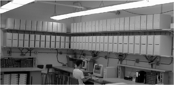
Figure 2.: The asteroseismology metacomputer, a collection of 64 minimal PCs connected by a network, which we used to perform the calculations in parallel.

We call this new instrument Darwin. It consists of 64 minimal PCs connected by a network, and can compute our models in parallel with a speedup factor of about 60 (see Metcalfe & Nather 1999a,b). Each box contains only a processor, 32 Mb of memory, and an ethernet card with a custom Linux bootrom.

2.3. Proof of Principle

Once our code was running on this machine, the first thing we did was generate a set of pulsation periods from a model within the search space, and then let the GA try to find the input parameters.

In 9 out of 20 runs using different random number sequences, the GA found the exact answer. In an additional 4 runs, it ended up with an answer close enough to the correct one for a small grid to yield the exact answer. This means that for a given run, there is a 35% chance that we won’t find the right answer, but if we perform 5 independent runs there will be a 99% probability of finding the right answer.

Next, we added noise to the input model to double check that the 5 run method was sufficient. We estimated the level of noise present on the observed frequencies in two ways. First, we used the identifications of the 63 linear combination frequencies (Vuille et al. 2000) to determine the distribution of differences between the observed and predicted frequencies. The best-fit Gaussian to this distribution had $\sigma=0.17~{}\mu$Hz. Second, we passed 100 synthetic light curves through a simulation of the standard WET reduction procedure, and looked at the distribution of differences between the input and output frequencies. This distribution was slightly narrower, having a best-fit Gaussian with $\sigma=0.053~{}\mu$Hz. We ran the GA method on several realizations of each estimate of the noise, and in all cases it found the right answer.

3. Results

Finally, we applied the new method to the real data for GD 358. To facilitate comparison with earlier work we ran the GA on six different combinations of core composition and transition profiles: pure carbon, pure oxygen, and mixed 50:50 & 20:80 C/O cores with both “steep” and “shallow” transition profiles (see Bradley Winget & Wood 1993).

The first thing we noticed was that there were two families of solutions in the larger search space, corresponding to thick and thin helium layers. These two families did not contain equally good solutions—one was always clearly better than the other—but which family was preferred depended on the core composition. Notably, when we restricted the GA to looking in the region of parameter-space searched by Bradley & Winget, it found the same answer that they found.

In general, reasonably good fits were possible for every core composition, but excellent fits were only possible in one specific case: the 20:80 C/O “shallow” mix. This new best-fit model is shown in the top panel of Figure 3 with the solution of Bradley & Winget shown in the bottom panel for comparison. The root-mean-square (r.m.s.) period difference between the new best-fit model and the observations is 1.50 seconds, compared to 2.69 seconds for Bradley & Winget’s solution. The second best fit found by the GA had an r.m.s. of 1.76 seconds—significantly worse considering that the noise on the individual periods amounts to only a few hundredths of a second.

Figure 3.: The observed periods and period-spacing for GD 358 (solid points) with the best-fit models (open points) from (a) the genetic algorithm, and (b) Bradley & Winget (1994).

4. Future Work

Although the new best-fit model is significantly better than the previous solution, it clearly still needs improvement. It’s possible that the duality between thick and thin helium layers for GD 358 is an indication that composition transitions exist in both places. This idea has been followed up in the context of possible ³He diffusion by Montgomery Metcalfe & Winget in these proceedings.

Another possibility is that more realistic C/O transition profiles, such as those of Salaris et al. (1997), will provide the extra structure needed by the models to fit the observed data. Combining the use of these profiles with a treatment of the central oxygen abundance as a free parameter by the GA, we can realistically expect to measure the central C/O ratio in GD 358. During helium burning the ${}^{12}{\rm C}(\alpha,\gamma)^{16}{\rm O}$ and the $3\alpha$ reactions are competing for the available $\alpha$-particles, so the final carbon to oxygen ratio in the core provides a direct measure of the relative rates of these two reactions (Buchman 1996). This is especially significant considering the difficulty of measuring the ${}^{12}{\rm C}(\alpha,\gamma)^{16}{\rm O}$ reaction in the laboratory.

Finally, we may be able to reverse-engineer the shape of the C/O transition profile by parameterizing the Brunt-Väisälä frequency and investigating what changes to the shape yield significantly better fits to the data. This would provide an independent check on the theoretical profiles, and would open up an entirely new approach to improving our models.

Acknowledgments.

I would like to thank Ed Nather and Don Winget for their guidance; Mike Montgomery, Paul Bradley, S.O. Kepler and Craig Wheeler for helpful discussions; Paul Charbonneau for supplying an unreleased version of the PIKAIA genetic algorithm; and Gary Hansen for arranging the donation of 32 computer processors through AMD.

References

Beauchamp, A., Wesemael, F., Bergeron, P., Fontaine, G., Saffer, R. A., Liebert, J. & Brassard, P. 1999, ApJ, 516, 887

Bradley, P. A. 1993, Ph.D. thesis, University of Texas-Austin

Bradley, P. A. & Winget, D. E. 1994, ApJ, 430, 850

Bradley, P. A., Winget, D. E. & Wood, M. A. 1993, ApJ, 406, 661

Buchman, L. 1996, ApJ, 468, L127

Metcalfe, T. S., & Nather, R. E. 1999a, Linux Journal, 65, 58

Metcalfe, T. S., & Nather, R. E. 1999b, Baltic Astronomy, 8, in press

Napiwotzki, R., Green, P. J. & Saffer, R. A. 1999, ApJ, 517, 399

Nather, R.E., Winget, D.E., Clemens, J.C., Hansen, C.J. & Hine, B.P. 1990, ApJ, 361, 309

Salaris, M., Dominguez, I., Garcia-Berro, E., Hernanz, M., Isern, J. & Mochkovitch, R. 1997, ApJ, 486, 413

Vuille, F., O’Donoghue, D., Buckley, D.A.H., Massacand, C., Solheim, J.E., Bard, S., Vauclair, G., Giovannini, O., Kepler, S.O., Kanaan, A., Provencal, J.L., Wood, M.A., Clemens, J.C., Kleinman, S.J., O’Brien, M.S., Nather, R.E., Winget, D.E., Nitta, A., Klumpe, E.W., Montgomery, M.H., Watson, T.K., Bradley, P.A., Sullivan, D.J., Wu, K., Marar, T.M.K., Seetha, S., Ashoka, B.N., Mahra, H.S., Bhat, B.C., Babu, V.C., Leibowitz, E.M., Hemar, S., Ibbetson, P., Mashals, E., Meistas, E., Moskalik, P., Zola, S., Krzesiński, J. & Pajdosz, G., 2000, MNRAS, 314, 689

Winget, D.E., Nather, R.E., Clemens, J.C., Provencal, J.L., Kleinman, S.J., Bradley, P.A., Claver, C.F., Dixson, J.S., Montgomery, M.H., Hansen, C.J., Hine, B.P., Birch, P., Candy, M., Marar, T.M.K., Seetha, S., Ashoka, B.N., Leibowitz, E.M., O’Donoghue, D., Warner, B., Buckley, D.A.H., Tripe, P., Vauclair, G., Dolez, N., Chevreton, M., Serre, T., Garrido, R., Kepler, S.O., Kanaan, A., Augusteijn, T., Wood, M.A., Bergeron, P. & Grauer, A.D. 1994, ApJ, 430, 839