A moving cold front in the intergalactic medium of A3667.

Abstract

We present results from a Chandra observation of the central region of the galaxy cluster A3667, with emphasis on the prominent sharp X-ray brightness edge spanning 0.5 Mpc near the cluster core. Our temperature map shows large-scale nonuniformities characteristic of the ongoing merger, in agreement with earlier ASCA results. The brightness edge turns out to be a boundary of a large cool gas cloud moving through the hot ambient gas, very similar to the “cold fronts” discovered by Chandra in A2142. The higher quality of the A3667 data allows the direct determination of the cloud velocity. At the leading edge of the cloud, the gas density abruptly increases by a factor of $3.9\pm 0.8$, while the temperature decreases by a factor of $1.9\pm 0.2$ (from 7.7 keV to 4.1 keV). The ratio of the gas pressures inside and outside the front shows that the cloud moves through the ambient gas at near-sonic velocity, $M=1\pm 0.2$ or $V=1400\pm 300$ km s^-1. In front of the cloud, we observe the compression of the ambient gas with an amplitude expected for such a velocity. A smaller surface brightness discontinuity is observed further ahead, $\sim 350$ kpc in front of the cloud. We suggest that it corresponds to a weak bow shock, implying that the cloud velocity may be slightly supersonic. Given all the evidence, the cold front appears to delineate the remnant of a cool subcluster that recently has merged with A3667. The cold front is remarkably sharp. The upper limit on its width, $3.5^{\prime\prime}$ or 5 kpc, is several times smaller than the Coulomb mean free path. This is a direct observation of suppression of the transport processes in the intergalactic medium, most likely by magnetic fields.

1 Introduction

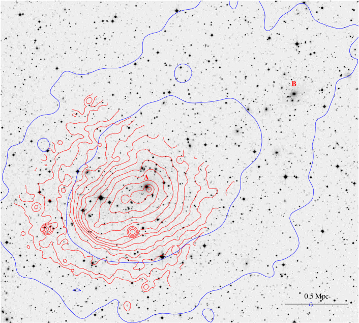
Abell 3667 manifests itself in the optical, X-rays, and in the radio as a spectacular ongoing merger. The cluster optical morphology is bimodal, with prominent galaxy concentrations around the two brightest galaxies (Sodre et al. 1992). It is likely that these two concentrations (called subclusters A and B below, see Fig. 1) correspond to the colliding subclusters. The line-of-sight velocity difference of the dominant galaxies is only 120 km s^-1 (Katgert et al. 1998). Since the merger velocities are expected to be in the range of a few thousand km s^-1, the small velocity difference between the dominant galaxies strongly suggests that the merger axis is nearly perpendicular to the line of sight. Bimodal cluster structure also is evident in the weak lensing mass map (Joffre et al. 2000). The ROSAT PSPC image (Knopp, Henry & Briel 1996, blue contours on Fig. 1) suggests an ongoing merger. The diffuse X-ray emission peaks on the main subcluster and has a general extension towards the smaller subcluster. In the cluster outskirts, the merger probably gives rise to the acceleration of relativistic electrons responsible for the Mpc-scale radio halo (Röttgering et al. 1997).

The most striking feature in the X-ray surface brightness distribution, apparent already in the ROSAT PSPC and HRI images, is a sharp arc-like discontinuity in the X-ray surface brightness distribution to the South-East of subcluster A and oriented approximately perpendicular to the line connecting subclusters A and B (Markevitch, Sarazin & Vikhlinin 1999). The sharpness of this discontinuity led Markevitch et al. to suggest that it was a shock front, even though the coarse ASCA temperature map was not entirely consistent with the shock explanation.

The study of this surface brightness edge was the main goal of our Chandra observation described here. This observation leads to the unexpected conclusion that the brightness discontinuity is not a shock front, but the leading edge of a large body of the cool dense gas moving through the hotter gas, very much like the two structures found with Chandra in A2142 (Markevitch et al. 2000). To reflect the nature of the surface brightness edge, we will call it a cold front. The high quality of the Chandra data allows a detailed investigation of the cold front and its vicinity. We show that the dense gas body moves in the hot ambient gas at nearly the velocity of sound of that gas (§ 5.1). We also observe a compression of the hot gas in front of the cloud (§ 5.3), and further ahead, a possible bow shock (§ 5.2). Both these features are expected to be present in front of a high-velocity cloud. We show that the front width is smaller than the particle Coulomb mean free path (§ 5.4), and speculate that the diffusion across the front should be suppressed by formation of a magnetic layer. In the accompanying paper (Vikhlinin et al. 2000), we use the apparent dynamical stability of the front to derive the strength of the magnetic field in this layer.

Figure 1: Chandra and ROSAT X-ray contours overlayed on the optical Digitized Sky Survey-II image. Note that the bright point source near galaxy A is associated with a faint point-like optical source and not with the galaxy. North is up and East is to the left, as they are in all other images.

We use $H_{0}=50$ km s^-1 Mpc^-1 and $q_{0}=0.5$, which corresponds to the linear scale of 1.46 kpc/arcsec at the cluster redshift $z=0.055$.

2 Data Reduction

A3667 was observed by Chandra with the ACIS-I detector in a single 49 ksec observation on Sept 22, 1999, soon after the degradation of the front-illuminated CCDs has stopped. The data were telemetered in Very Faint mode. The average total count rate during the quiescent background intervals, 67.1 cnt s^-1, was only slightly below the telemetry saturation limit of $\sim 69$ cnt s^-1 in this mode. This resulted in data drop-outs during periods of high background. Fortunately, these periods were isolated in time and affected only a small fraction of the exposure. We excluded the time intervals when the telemetry was missing in any of the four ACIS-I CCDs, 6 ksec in total. The remaining 43 ksec of the observation were not affected by background flares or any other problem.

The standard screening was applied to the photon list, omitting ASCA grades 1, 5, and 7, known hot pixels, bad columns, and chip node boundaries. The clean photon list was reprocessed using the latest available calibration to correct for position-dependent gain variations due to the CTI effect.

The analysis of extended sources requires a careful background subtraction. Since the particle background on ACIS-I is spatially non-uniform, and also because A3667 fills the entire field of view, it was necessary to use an external dataset for background subtraction. The background dataset was prepared using a procedure described by Markevitch et al. (2000) from a collection of blank field observations with a total exposure of 300–400 ksec, depending on the CCD chip (Markevitch 2000). The accuracy of the background subtraction was checked using the data at high energies, where the cluster emission is negligible compared to the background (10–11 keV in the ACIS-I chips and 5–11 keV in the off-axis ACIS-S2 chip where the cluster surface brightness is much lower). We found that the background normalization should be increased by 7%, within the suggested 10% uncertainty and consistent with the possible long-term trend (Markevitch 2000). Therefore, in the rest of the analysis, we have increased the background normalization by 7% at all energies. All the confidence intervals reported below include the $\pm 10\%$ systematic uncertainty we allow for the background normalization.

The imaging analysis has been performed in the 0.5–4 keV energy band to maximize the source-background ratio. The background-subtracted images were corrected for vignetting and exposure variations.

Because of the CTI effect, the quantum efficiency of the ACIS-I CCDs at high energies strongly depends on the distance from the chip readout. For example, the quantum efficiency at 6 keV decreases by $\sim 20\%$ at readout distances greater than $1/3$ of the CCD size. Our spectral analysis uses approximate position-dependent corrections to the quantum efficiency which were determined using observations of the supernova remnant G21.5–0.9 and the Coma cluster (Vikhlinin 2000). For spectra extracted in large regions, the position-dependent spectral response matrices and effective area functions were weighted with the cluster flux.

To check the validity of the calibration relevant to the spectral analysis, we compared the values of cluster temperature measured with Chandra and ASCA. The integrated Chandra spectrum is well fit by a Raymond-Smith model with temperature $T=7.31\pm 0.17$ keV, heavy metal abundance $a=0.31\pm 0.03$, and absorption $N_{H}=(4.1\pm 0.3)\times 10^{20}\,$cm^-2 (all uncertainties are at the 68% confidence level). The derived temperature is in agreement with the ASCA value, $T=7.0\pm 0.4$ keV (Markevitch et al. 1998), and the absorption is reasonably consistent with the Galactic value, $N_{H}=4.8\times 10^{20}\,$cm^-2.

Figure 2: Smoothed 0.5–4 keV Chandra image (full $16^{\prime}\times 16^{\prime}$ ACIS-I field of view; North is up, East is to the left). The most prominent feature is the sharp surface brightness edge (cold front). The front shape is nearly circular as indicated by the arc. The sector to the South-East of the center of curvature of the edge (its location denoted with an $\times$) was used for the surface brightness and temperature profile measurements. The two segments on both sides of the possible bow shock indicate the regions where the temperature was measured (§ 5.2).

Figure 3: (a) Photon image in the 0.5–4 keV band binned to $2^{\prime\prime}$ pixels. (b) Temperature map. The corners are not shown due to poor statistics. The typical statistical error in this image is $\pm 1$ keV. The cold, $\sim 4$ keV, region near the center of the map coincides with the inside of the surface brightness edge. The very high temperature in several spots just outside the edge is insignificant. All other temperature variations greater than $\pm 1$ keV are significant.

2.1 Temperature Map Determination

The Chandra angular resolution, in principle, allows a straightforward spectral modeling in very small (a few arcsec) regions, limited only by statistics. Our technique for temperature map determination closely follows that of Markevitch et al. (2000). We extracted images in 11 energy bands, 0.7–1.15–1.6–2.5–3–3.5–4.25–5–6–7–8–9 keV bands, subtracted the background, masked point sources, and smoothed the images with a variable-width Gaussian filter. The Gaussian filter width was $\sigma=48^{\prime\prime}$ everywhere, except for a narrow region near the surface brightness edge, where the filter width was smoothly reduced to $\sigma=24^{\prime\prime}$. We also appropriately weighted the statistical uncertainties to determine the noise in the smoothed images. The effective area as a function of energy at each point was calculated as the product of the position-dependent CCD quantum efficiency and mirror vignetting. Finally, we generated the response matrices from the position-dependent calibration data and determined the temperature by fitting these 11 energy points to a single-temperature plasma model with absorption fixed at the Galactic value and the heavy element abundance fixed at the best-fit cluster average.

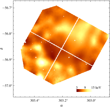
3 Overview of the X-ray Image and Temperature Map

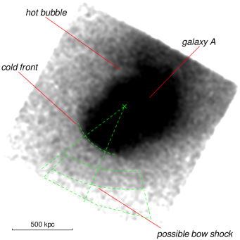
The Chandra image reveals interesting structures in the central part of A3667. The features discussed below are indicated in the smoothed image (Fig. 2). The most prominent feature in this image — and the main subject of our further investigation — is the sharp edge in the surface brightness distribution to the South-East of galaxy A. The edge is even more impressive in the raw photon image (Fig. 3). The edge is located approximately 550 kpc to the South-East of galaxy A, and it is almost perpendicular to the line connecting subclusters A and B (Fig. 1). Its morphology suggests motion to the South-East, away from galaxy A. Our temperature map shows that the gas is cooler on the brighter (denser) side of the edge, which rules out a shock front interpretation. A detailed analysis of the temperature and density profiles across this “cold front” presented below (§ 4) shows unambiguously that this is a cold gas body moving to the South-East at a slightly supersonic speed.

Farther South-South-East of galaxy A, approximately 300 kpc beyond the cold front, there is a weaker discontinuity in the surface brightness distribution (Fig. 2). We argue in § 5.2 that this discontinuity may correspond to a bow shock in front of the supersonically moving cold gas cloud.

Figure 4: (a): X-ray surface brightness profile (expressed in the units of energy flux in the 0.5–2 keV band) across the cold front. The profile was measured in the sector shown in Fig. 2. The Chandra photon flux in the 0.5–4 keV band was converted to an energy flux in the 0.5–2 keV band. The distance is measured relative to the front position. The dashed line shows the ROSAT PSPC $\beta$-model fit (no renormalization applied) to the profile in the outer part of the cluster. The dotted line shows the fit to the projected spheroidal density discontinuity model (see text). (b): Temperature profile across the front measured in the same sector as the surface brightness profile. The dashed lines show the adopted mean gas temperature inside and outside the front (see text).

Two additional structures in the temperature map are noteworthy, although they are not the focus of this paper. The temperature map reveals a hot (11 keV) region immediately North-West of galaxy A. This region coincides with the X-ray surface brightness extension connecting subclusters A and B. Most likely, the gas in this region is heated by shocks generated by the merger.

The hot region has an extension at approximately 300 kpc to the North-East of galaxy A. The extension is almost perpendicular to the merger axis and coincides with a region of decreased surface brightness, which indicates low gas density. Such structures can be generated by shock heating of the gas between the colliding subclusters. If shock heating is strong enough, the gas specific entropy in this region can be increased so that the gas becomes convectively unstable. This will result is formation of hot underdense gas bubbles rising buoyantly along the gradient of the gravitational potential, i.e. perpendicular to the merger axis, which is what we may be seeing.

Finally, we note that the Chandra temperature map reasonably agrees in the overlapping region with the coarser ASCA temperature map presented in Markevitch et al. (1999).

4 Structure of the Cold Front

In the position angle interval 200°–260° (the position angles are measured from West through North hereafter) from the galaxy A, where the surface brightness discontinuity is most prominent (Fig. 2), the isophote of the edge is very well fit by a circle with a radius $410\pm 15$ kpc and a centroid located $\sim 200$ kpc East-South-East of galaxy A. The abrupt increase in the X-ray brightness suggests the presence of a dense gas body with a sharp boundary. Since the surface brightness edge is nearly circular and since the merger appears to proceed in the plane of the sky, we can assume that the 3-dimensional shape of the gas body is reasonably close to a spheroid with the axis of symmetry in the plane of the sky. These assumptions allow us to derive the gas density within the body by deprojecting the X-ray surface brightness profile across the edge.

The X-ray surface brightness and temperature profiles across the edge are shown in Fig. 4. They were measured in the 215°–245° sector shown in Fig. 2. As we cross the edge from the outside, the surface brightness increases sharply by a factor of 2 within 7–10 kpc and continues to increase smoothly by another factor of 2 within 40–80 kpc. Such a profile suggests a projected density discontinuity, and is, indeed, well fit by the model of a projected spheroid. The surface brightness profile of a spheroid with a constant gas density is given by

$$S(d)=2^{3/2}\sqrt{R}\,\varepsilon_{0}\;\sqrt{d}\qquad\mbox{for $d\ll R$},$$ (1)

where $d$ is the distance from the edge, $\varepsilon_{0}$ is the volume emissivity of the gas, and $R$ is the radius of curvature of the front (see Appendix). We add to this equation a component that corresponds to the projection of the ambient gas. This component is small and nearly constant, $\approx 4.5\times 10^{-13}$ erg s${}^{-1}\,$cm^-2 arcmin^-2. As Figure 4 shows, this model provides an excellent fit to the surface brightness within $100$ kpc interior to the edge. The model can be generalized by using a power law gas density distribution within the spheroid, $\rho=\rho_{0}(x^{2}/b^{2}+y^{2}/a^{2})^{-3\beta/2}$. The surface brightness profile in this case is given by eq. (A4). The fit of this equation to the observed profile 80 kpc interior to the front gives $\beta=0.07\pm 0.08$ (68% confidence). Therefore, the gas distribution is consistent with a step-like jump in the density and with a constant density inside the front. The normalization of the fit provides the electron density inside the front $n_{e}=(3.2\pm 0.09)\times 10^{-3}\,$cm^-3, where the uncertainty is due to statistics and the poorly constrained power-law density slope. A larger contribution to the density uncertainty is the unknown elongation of the gas cloud along the line of sight. Equation (A6) shows that if the spheroidal cloud is elongated by a factor of $1+e$ along the line of sight, the gas density that is needed to reproduce the observed profile decreases as $(1+e)^{-1/2}$. An elongation $|e|>0.3$ appears unlikely because it would be perpendicular to the merger axis and because the front shape in projection is nearly circular. Therefore, the density uncertainty on the inner side of the front due to the cloud elongation should be within $\approx e/2=\pm 15\%$; this uncertainty is adopted in the discussion below.

The gas density on the outer side of the front was derived using the ROSAT PSPC image because the Chandra field of view is too small to permit a proper deprojection of the slowly varying surface brightness in this region. The ROSAT isophotes are nearly circular in the South-Eastern sector of the cluster (Knopp et al. 1996; Fig. 1), which suggests that this sector is not significantly disturbed by the merger. Therefore, the gas density can be derived by the standard approach assuming spherical symmetry. The ROSAT surface brightness profile was extracted in the sector 160°–250° centered on galaxy A and fit with a $\beta$-model, $I=I_{0}/(1+r^{2}/r_{c}^{2})^{3\beta-0.5}$, in the radial range 0.6–3.5 Mpc (i.e., from just outside the front to the edge of the ROSAT field of view). The $\beta$-model provides a good fit to the data; the best fit parameters are $\beta=0.79$, $r_{c}=690$ kpc, and $I_{0}=0.0120$ cnt s^-1 arcmin^-2 in the 0.7–2 keV energy band. This fit is in excellent agreement with the Chandra surface brightness at distances greater than 70 kpc of the edge, with no renormalization required (Fig. 4). Just outside the front, the $\beta$-model fit gives the electron density $n_{e}=0.82\times 10^{-3}\,$cm^-3. Although the $\beta$-model parameters are quite sensitive to the choice of the profile centroid, the density at the edge position is not. For example, if the profile is centered at a point in the middle of the front, we obtain $\beta=0.73$, $r_{c}=600$ kpc, $I_{0}=2.91\times 10^{-3}\,$cnt s^-1 arcmin^-2, and the electron density near the front is $n_{e}=0.80\times 10^{-3}\,$cm^-3.

We note that the surface brightness within $\sim 70$ kpc exterior to the front exceeds both the ROSAT model and the extrapolation of the Chandra profile from larger radii. Our interpretation of the observed density edge as a boundary of a fast-moving dense gas body predicts just such a compression in the immediate vicinity of the front. This is discussed in more detail in § 5.3. Our immediate purpose — calculation of the cloud velocity — requires a measurement of the undisturbed (free stream) gas density on the outer side of the front. One approach to derive the free stream density is to use the density just outside the compression region, at $d\approx-100$ kpc. The ROSAT $\beta$-model gives $n_{e}=0.71\times 10^{-3}\,$cm^-3 at this distance. A better approach is to extrapolate the $\beta$-model to the front position because it approximately accounts for the small change in the global cluster gravitational potential. Our discussion below uses the value $n_{e}=0.82\times 10^{-3}\,$cm^-3 obtained by extrapolating the ROSAT model to the front position. We allow a $15\%$ uncertainty in this value.

As we cross the edge from the outside, the temperature changes abruptly from approximately 8 keV to 4–5 keV (Fig. 4). On both sides, the temperature is consistent with a constant value within some distance of the front. The fit to the spectra integrated within 275 kpc beyond and 125 kpc behind the front are $T_{\rm out}=7.7\pm 0.8$ keV and $T_{\rm in}=4.1\pm 0.2$ keV, respectively. We will adopt these values as the gas temperature outside and inside the dense cloud.

The temperature in a 10 kpc strip just inside the front, $5.1\pm 0.7$ keV, is marginally higher than the average inner temperature. Because of the curvature of the front along the line of sight, this annulus is significantly affected by projection, with 30–50% of the emission being due to the ambient 8 keV gas. The two-temperature fit in this region, with the temperature of the hotter component fixed at 8 keV and a normalization of 50% that of the colder, component gives a temperature for the colder component of $T=3.7\pm 0.7$ keV, which is consistent with the value at larger distances from the edge. Therefore, the marginal increase of temperature just inside the front is consistent with projection and does not require, for example, heat conduction.

In summary, both the density and temperature of the gas change abruptly as we cross the boundary of the dense cloud.

Table 1: Gas parameters in several regions

Region	$T$	$n_{e}$	$p=Tn_{e}$
	keV	$10^{-3}\,$cm-3	$10^{-2}\,$keV cm-3
Outside the front	$7.7\pm 0.8$	$0.82\pm 0.12$	$0.63\pm 0.11$
Inside the front	$4.1\pm 0.2$	$3.2\pm 0.5$	$1.32\pm 0.21$
Inside bow shock	$8.2\pm 0.9$	$\cdots$	$\cdots$
Outside bow shock	$7.7\pm 1.2$	$\cdots$	$\cdots$

5 Discussion

Let us consider the pressures on the two sides of the cold front. If the dense gas cloud were at rest relative to the hot gas, the pressures would be equal on both sides. However, we observe a jump by a factor of $2.09\pm 0.48$ (Table 4). The most natural explanation would be that the cloud moves through the ambient gas and is subject to its ram pressure in addition to thermal pressure. From our data, we can determine the velocity required to produce the additional pressure. Because of the simple geometry, the gas flow in our case can be approximated by the flow of uniform gas about a blunt body of revolution. Figure 5 shows several characteristic regions in such a flow. Far upstream from the body, the gas is undisturbed and flows freely. This region is referred to as the free stream; in the discussion below, we use an index 1 for gas parameters in this region. Near the leading edge of the body, the gas decelerates approaching zero velocity at the leading edge. This region is referred to as the stagnation point; we will use an index 0 for gas parameters in this region. If the velocity of the body exceeds the speed of sound, a bow shock forms at some distance upstream from the body. The gas parameters just inside the bow shock will be denoted with an index 2. Finally, the gas parameters inside the cloud will have index $0^{\prime}$.

All these regions are seen in the Chandra observation of A3667. In § 5.1, we determine the velocity of the dense cloud from the ratio of gas pressures in the free stream and inside the front. The cloud velocity turns out to be very close to the velocity of sound in the ambient gas. In § 5.2, we discuss the possible bow shock. The gas density in front of the fast moving cloud should be significantly higher than in the free stream. We show in § 5.3 that this compression is indeed seen in the Chandra image.

Most of the further discussion assumes that the gas flow outside the cloud is adiabatic, i.e., that heat conduction can be neglected. We generally consider length scales much greater than the Coulomb mean free path; heat conduction is slower than the gas motions on such scales. Also, and perhaps more important, heat conduction is likely strongly suppressed by the presence of magnetic fields.

Figure 5: Geometry of flow past a spheroid with semi-axes $a$ and $b$. Zones 0, 1, and 2 are those near the stagnation point, in the undisturbed free stream, and past the possible bow shock, respectively. Zone $0^{\prime}$ is within the body.

Figure 6: Ratio of pressures at the stagnation point and in the free stream as a function of the Mach number in the free stream. The solid and dashed line corresponds to the sub- and supersonic regimes (eqs. 2, 3), respectively. The dotted lines show the conservative confidence interval for the measured pressure ratio.

5.1 Velocity of the Hot Gas Cloud

The ratio of pressures in the free stream and at the stagnation point is a function of the cloud speed $V$ (Landau & Lifshitz 1959, § 114):

$$\frac{p_{0}}{p_{1}}=\left(1+\frac{\gamma-1}{2}\;M_{1}^{2}\right)^{\frac{\gamma}{\gamma-1}},\quad M_{1}\leq 1$$ (2)

$$\frac{p_{0}}{p_{1}}=\left(\frac{\gamma+1}{2}\right)^{\frac{\gamma+1}{\gamma-1}}M_{1}^{2}\left[\gamma-\frac{\gamma-1}{2M_{1}^{2}}\right]^{-\frac{1}{\gamma-1}},\quad M_{1}>1,$$ (3)

where $M_{1}=v/c_{1}$ is the Mach number in the free stream and $\gamma=5/3$ is the adiabatic index of the monatomic gas. The subsonic equation (2) follows from Bernoulli’s equation. The supersonic equation (3) is more complex because it accounts for the gas entropy jump at the bow shock. Figure 5 illustrates that $p_{0}/p_{1}$ is a strong function of the cloud velocity; therefore the cloud velocity can be measured rather accurately even if the pressure uncertainties are relatively high.

The gas parameters at the stagnation point — which enter eq. (2)–(3) — cannot be measured directly because the stagnation region is physically small and therefore its X-ray emission is almost completely hidden by projection. However, the gas pressure at the stagnation point must equal the pressure within the cloud, $p_{0^{\prime}}$, which is well-determined. The conservative confidence interval of the pressure ratio $p_{0^{\prime}}/\!p_{1}=2.09\pm 0.48$ corresponds to $M_{1}=1.0\pm 0.2$, i.e. the gas cloud moving at the sound speed of the hotter gas. The cloud velocity in physical units is $V=M_{1}c_{1}=M_{1}\sqrt{\gamma T/m_{p}\mu}=1430\pm 290$ km s^-1, where we used the gas temperature $T=7.7$ keV and the mean molecular weight of the intracluster plasma $\mu=0.6$.

5.2 Possible Bow Shock

If the speed of a blunt body exceeds the speed of sound, a bow shock forms at some distance upstream. A surface brightness discontinuity resembling a bow shock is indeed visible in the Chandra image at $\sim 350$ kpc from the cold front (Fig. 2). The shape of this structure is consistent with an ellipse centered on the center of curvature of the cold front. The surface brightness profile extracted in concentric elliptical annuli in the position angle range 230°–280° (Fig. 5.2) shows an increase in the surface brightness by a factor of 1.25 within a narrow radial range around $\sim 350$ kpc from the cold front. This corresponds to a gas density jump by a factor of $1.1-1.2$, depending on the projection geometry. If this discontinuity is interpreted as a shock front, it is straightforward to derive the expected temperature jump, the shock propagation velocity, and the velocity of the gas behind the shock, using the Rankine-Hugoniot shock adiabat (Landau & Lifshitz, § 85). For this weak shock with $\rho_{2}/\rho_{1}=1.1-1.2$, the propagation velocity should be close to the velocity of sound in the pre-shock gas, or more exactly, $1.07-1.13$ of that velocity. The temperature ratio expected for the shock with such a density jump is $T_{2}/T_{1}=1.07-1.13$. This is consistent with the measured values of $T_{2}=8.2\pm 0.9$ keV and $T_{1}=7.7\pm 1.2$ keV derived in regions shown in Fig. 2. Evaluating the pre-shock sound velocity from $T_{1}=7.7$ keV, we find the shock propagation velocity $V\approx 1600$ km s^-1. As expected for a stationary shock, this value agrees with the velocity of the cold cloud derived from independent considerations.

The observed distance between the shock and the cold front agrees well with that expected for this velocity. The distance between the bow shock and a blunt body can be found using the approximate method of Moeckel (1949; see also Shapiro 1953). The shape of the cold gas cloud in A3667 can be approximated by a cylinder with diameter $D\sim 500$ kpc and a spherical head with radius $R=410$ kpc seen as the front in the projection. For this geometry, Moeckel’s method predicts a bow shock distance of 560–320 kpc for Mach numbers $M_{1}=1.05-1.2$. Thus the observed distance of 350 kpc corresponds to a Mach number in the correct range.

We note that the shock-like feature is observed only in the Southern region of the image and is not symmetric relative to the presumed direction of the cloud motion. Since the motion is only slightly supersonic, small-amplitude temperature nonuniformities can make it subsonic in certain regions and a shock will not arise everywhere. Another possible explanation is that nontrivial projection effects mask the shock.

Figure 7: X-ray surface brightness profile across the possible bow shock. The profile has been measured in a sector defined by the two segments in Fig. 2. The distance is measured from the cold front. The dotted line shows a fit to a model in which the gas density follows the power law with the same slope on both sides of the shock, and undergoes a jump by a factor of 1.15 at the position of the shock.

5.3 Stagnation Region

We now consider the region immediately in front of the dense cloud where the inflowing gas slows and hence its density rises, and show that this results in a detectable X-ray brightness enhancement. We will calculate the density enhancement with respect to either the free stream region, if the cloud motion is subsonic, or to the region just behind the bow shock, if the motion is supersonic. In both cases, the Mach number in the reference region is $M_{2}\leq 1$. The ratio of the gas density, $\rho$, at a point where the local Mach number of the flow is $M$, and the density in the reference region, $\rho_{2}$, is found from Bernoulli’s equation (e.g. Landau & Lifshitz, § 80), and then the enhancement of the X-ray emissivity, $\varepsilon$, is

$$\frac{\varepsilon}{\varepsilon_{2}}=\frac{\rho^{2}}{\rho_{2}^{2}}=\left(\frac{1+(\gamma-1)M^{2}/2}{1+(\gamma-1)M_{2}^{2}/2}\right)^{-2/(\gamma-1)}.$$ (4)

If $M_{2}=1$, the emissivity is enhanced by a factor of 2.4 at the stagnation point. The integration of eq. (4) along the line of sight gives the enhancement in the X-ray surface brightness. To carry out the integration, we need to know the gas velocity field. As a first approximation, we use the velocity field from the numerical simulation of an $M=1$ flow around a sphere by Rizzi (1980). For a sphere with radius $R=400$ kpc (the radius of curvature of the cold front) and the observed gas density, we find the surface brightness enhancement $\Delta S=2.3\times 10^{-14}\,$erg s^-1 cm^-2 arcmin^-2 with a characteristic width $\sim\!130$ kpc in the sky plane. Since the dense cloud is not a sphere, but rather a cylinder with diameter $D\approx 500$ kpc with a spherical head with $R=400$ kpc, the surface brightness enhancement has a smaller amplitude and width. The size of the compressed region along the line of sight is $\approx 2R$ in the case of a flow around a sphere. Therefore, for the real geometry, the amplitude of the surface brightness enhancement should be reduced by a factor $\sim D/2R=0.7$; the projected width of the compressed region is likely reduced by a similar factor. Therefore, we expect the surface brightness enhancement in front of the cloud to have an amplitude $1.6\times 10^{-14}\,$erg s^-1 cm^-2 arcmin^-2 and width $\sim 90$ kpc. Quite remarkably, we observe a surface brightness enhancement with similar parameters (Fig. 4).

The gas temperature in the stagnation region also should be higher than that in the free stream due to adiabatic compression. However, the temperature change is too weak to be detectable. The gas temperature in the adiabatic flow is proportional to $\rho^{\gamma-1}$. Using equation (4) one finds for $M_{2}=1$ that the temperature at the stagnation point is 33% higher than in the free stream. Since the stagnation region contributes only $\sim 30\%$ of the total X-ray brightness on the outer side of the front (Fig. 4), the projected temperature should increase by $\sim 10\%$, which is within the statistical uncertainties of our temperature measurement.

Figure 8: A detailed X-ray surface brightness profile near the edge position. The solid line shows the fit of the projected spherical density discontinuity with an infinitely small width. The dashed line corresponds to the projection of the same discontinuity smeared with the Gaussian $\sigma=20$ kpc.

5.4 Front Width and Suppression of the Transport Processes

The surface brightness edge is remarkably sharp. Indeed, with the Chandra angular resolution, we can tell that its width is smaller than the Coulomb mean free path of electrons and protons. Figure 5.3 shows a detailed X-ray surface brightness profile across the front. The surface brightness was measured in narrow $2.2\times 210$ kpc annular segments. The X-ray brightness increases sharply by a factor of 1.7 within only 2 kpc from the front position. We can compare this width with the Coulomb mean free path of electrons and protons in the plasma on both sides of the front. The Coulomb scattering of particles traveling across the front can be characterized by four different mean free paths: that of thermal particles in the gas on each side of the front, $\lambda_{\rm in}$ and $\lambda_{\rm out}$; and that of particles from one side of the front crossing into the gas on the other side, $\lambda_{\rm in\rightarrow out}$ and $\lambda_{\rm out\rightarrow in}$. From Spitzer (1962) we have for $\lambda_{\rm in}$ or $\lambda_{\rm out}$:

$$\lambda=15~{}{\rm kpc}\left(\frac{T}{7~{}{\rm ke\kern-0.50003ptV}}\right)^{2}\left(\frac{n_{e}}{10^{-3}~{}{\rm cm}^{-3}}\right)^{-1},$$ (5)

and for $\lambda_{\rm in\rightarrow out}$ and $\lambda_{\rm out\rightarrow in}$:

$$\lambda_{\rm in\rightarrow out}=\lambda_{\rm out}\,\frac{T_{\rm in}}{T_{\rm out}}\,\frac{G(1)}{G(\sqrt{T_{\rm in}/T_{\rm out}})}$$ (6)

$$\lambda_{\rm out\rightarrow in}=\lambda_{\rm in}\,\frac{T_{\rm out}}{T_{\rm in}}\,\frac{G(1)}{G(\sqrt{T_{\rm out}/T_{\rm in}})},$$ (7)

where $G(x)=(\Phi(x)-x\Phi^{\prime}(x))/2x^{2}$ and $\Phi(x)$ is the error function. Using the gas parameters on the two sides of the front (Table 4), we find the numerical values $\lambda_{\rm out}=22$ kpc, $\lambda_{\rm in}=1.6$ kpc, $\lambda_{\rm in\rightarrow out}=13$ kpc, $\lambda_{\rm out\rightarrow in}=3.5$ kpc.

The hotter gas in the stagnation region has a low velocity relative to the cold front. Therefore, diffusion, which is undisturbed by the gas motions, should smear any density discontinuity by at least several mean free paths on a very short time scale. Diffusion in our case is mostly from the inside of the front to the outside, because the particle flux through the unit area is proportional to $nT^{1/2}$. Thus, if Coulomb diffusion is not suppressed, the front width should be at least several times $\lambda_{\rm in\rightarrow out}$. Such a smearing is clearly inconsistent with the sharp rise in the X-ray brightness interior to the front (Fig. 5.3). An upper limit on the front width can be determined by fitting the observed surface brightness profile with a model of the projected spherical density discontinuity whose boundary (in 3D) is smeared with a Gaussian $\exp(-r^{2}/2\sigma^{2})$. The best fit model (solid line in Fig. 5.3) requires $\sigma=0$. The formal 95% upper limit on $\sigma$ is only 5 kpc. This can be explained only if the diffusion coefficient is suppressed by at least a factor of 3–4 with respect to the Coulomb value.

The suppression of transport processes in the intergalactic medium is usually explained by the presence of a magnetic field. The suppression is effective if the magnetic field lines are either strongly tangled or there is a large-scale field perpendicular to the direction in which diffusion or heat conduction is to occur. If the magnetic field is tangled, the observed width of the front, $\sigma<5$ kpc, is the upper limit on the magnetic loop size. The other possibility is that the magnetic field is mostly parallel to the front at least in a narrow layer. In the subsequent paper (Vikhlinin et al. 2000), we show that the existence of such a parallel component in the magnetic field is required for dynamical stability of the front. Such a component would provide effective isolation of the cold gas cloud and prevent the observed sharp density gradient from dissipating.

6 Summary

The analysis of Chandra observation of A3667 presented here leads to the following conclusions:

1. The prominent sharp discontinuity in the X-ray surface brightness distribution spanning 0.5 Mpc around the South-Eastern side of one of the two subclusters, is not a shock front as proposed before, but instead a “cold front”, i.e., a boundary of a dense cool gas body embedded in the hotter ambient gas.

2. The gas pressure inside the cloud is $2.1\pm 0.5$ times higher than that in the ambient gas. The higher pressure inside the cloud is most plausibly explained by the ram pressure caused by the motion of the cloud. The amplitude of the pressure jump requires near-sonic velocity of the cloud relative to the ambient gas (the Mach number is $M=1\pm 0.2$)

3. The near-sonic velocity of the cloud is independently confirmed by observation of compression of the ambient gas near the leading edge of the cloud, and by a possible bow shock seen $\sim 350$ kpc ahead of the cold front.

4. The width of the cold front is smaller than $3.5^{\prime\prime}$ or 5 kpc, which is a factor of 2–3 smaller than the Coulomb mean free path. This means that we directly observe the suppression of transport processes in the intergalactic medium, most likely by a magnetic field.

Appendix A Projection of the Spheroidal Gas Cloud

Projection of an abrupt density jump at the boundary of the spheroidal gas cloud results in a sharp elliptical edge in the surface brightness distribution. Here we calculate the expected surface brightness profile across this edge. The geometry of the problem and the notations are defined in Fig. 5. We assume the gas density near the spheroid boundary follows a power law

$$\rho(x,y)=\rho_{0}\left(\frac{x^{2}}{b^{2}}+\frac{y^{2}}{a^{2}}\right)^{-3\beta/2},$$ (A1)

where $\rho_{0}$ is the value at the boundary. The volume emissivity distribution is the square of the density distribution

$$\varepsilon=\varepsilon_{0}\left(\frac{x^{2}}{b^{2}}+\frac{y^{2}}{a^{2}}\right)^{-3\beta}.$$ (A2)

The line-of-sight distance through the spheroid, $l$, at the projected distance $d$ from the boundary is

$$l=a\,\left(1-\frac{(b-d)^{2}}{b^{2}}\right)^{1/2}=a\,\left(\frac{2d}{b}-\frac{d^{2}}{b^{2}}\right)^{1/2}.$$ (A3)

The surface brightness profile then is

$$S(d)=\int_{-l}^{l}\varepsilon\,dy=2a\varepsilon_{0}\;\left(\frac{2d}{b}-\frac{d^{2}}{b^{2}}\right)^{1/2}\;\times\;\left(\frac{b-d}{d}\right)^{-6\beta}\;{}_{2}\!F\!{}_{1}\left[\frac{1}{2},3\beta,\frac{3}{2};\frac{d(d-2b)}{(d-b)^{2}}\right],$$ (A4)

where ${}_{2}\!F\!{}_{1}$ is the hypergeometric function. The first factor in this equation, $2a\varepsilon_{0}\sqrt{2d/b-d^{2}/b^{2}}$, is the surface brightness profile expected for constant gas density, and the rest is the correction due to the power-law density distribution. For $|\beta|<0.25$, this correction factor can be adequately approximated as $(1-d/b)^{-3.45\beta}$.

We are interested in the surface brightness profile at distances $d$ small compared to the spheroid axis $b$. In this case, one can neglect the term $d^{2}/b^{2}$ under the square root as well as the correction due to the power law density profile. Equation (A4) then can be simplified to

$$S(d)\approx 2^{3/2}\sqrt{R}\,\varepsilon_{0}\;\sqrt{d}\qquad(d\ll b),$$ (A5)

where $R$ is the radius of curvature of the ellipse near the edge, $R=a^{2}/b$.

Finally, we should take into account a possible deviation of the gas cloud shape from the spheroid. A reasonable generalization is to assume that the cloud is ellipsoidal with one of the axes parallel to the line of sight. In this case, the semi-axis $a$ in eq. (A4) cannot be derived from observations. Instead, the shape of the surface brightness edge in projection defines $b$ and the third semi-axis, $a^{\prime}$. If we write $a=(1+e)a^{\prime}$, where $e$ is the unknown elongation of the cloud along the line of sight, eq. (A5) becomes

$$S(d)\approx 2^{3/2}(1+e)\sqrt{R_{1}}\,\varepsilon_{0}\;\sqrt{d}\qquad(d\ll b),$$ (A6)

where $R_{1}$ is the radius of curvature of the brightness edge in projection. Therefore, a projected ellipsoid should still have the characteristic square root surface brightness profile near the edge. The normalization of the profile depends only on the volume emissivity of the gas, the radius of curvature of the edge in projection, and on the elongation along the line of sight. Given the observed profile $S(d)$, the gas density is

$$\rho\approx\rho_{0}\propto\sqrt{\varepsilon_{0}}=2^{-3/4}\sqrt{S(d)}\;d^{-1/4}\times R_{1}^{-1/4}(1+e)^{-1/2}.$$ (A7)

It depends only weakly on the geometrical factors $R_{1}$ and $e$.