Secondary CMB Anisotropies from Cosmological Reionization

Abstract

We use numerical simulation of cosmological reionization to calculate the secondary CMB anisotropies in a representative flat low density cosmological model. We show that the kinetic Sunyaev-Zel’dovich effect (scattering off of moving electrons in the ionized intergalactic medium) is dominated by the nonlinear hydrodynamic and gravitational evolution of the density and velocity fields, rather than the detailed distribution of the ionization fraction (“patchy reionization”) on all angular scales. Combining our results with the recent calculation of secondary CMB anisotropies by Springel et al., we are able to accurately predict the power spectrum of the kinetic SZ effect on almost all angular scales.

1 Introduction

The reionization of the intergalactic medium (hereafter, IGM) stands out as one of the most important physical processes that have taken place in the early universe. Recent observational progress measuring the angular spectrum of anisotropies in the Cosmic Microwave Background radiation (hereafter CMB) on sub-degree angular scales (de Bernardis et al. 2000; Hanany et al. 2000), and in obtaining the absorption spectra of the most distant quasars (Stern et al. 2000; Zheng et al. 2000; Fan et al. 2000a) allows us to limit the redshift of reionization to somewhere between 6 and 30 (Griffiths, Barbosa, & Liddle 1998; Bond & Jaffe 1999; Tegmark & Zaldarriaga 2000). Combined with recent theoretical and numerical breakthroughs in our understanding how reionization proceeds in the inhomogeneous universe (Giroux & Shapiro 1996; Haiman & Loeb 1997; Gnedin & Ostriker 1997; Madau, Haardt, & Rees 1999; Miralda-Escudeé, Haehnelt, & Rees 1999; Ciardi et al. 1999; Valageas & Silk 1999; Chiu & Ostriker 2000; Gnedin 2000), these data finally place a study of reionization on much more solid footing.

Among the many effects of reionization, the secondary CMB anisotropies have been the subject of active study for a long time, beginning with the pioneering works of Ostriker & Vishniac (1986) and Vishniac (1987) and up to the most recent careful investigations (Hu & White 1996; Aghanim et al. 1996; Knox, Scoccimarro, & Dodelson 1998; Gruzinov & Hu 1998; Jaffe & Kamionkowski 1998; Peebles & Juszkiewicz 1998; Haiman & Knox 1999; Hu 2000; Bruscoli et al. 2000; da Silva et al. 2000; Refregier et al. 2000; Seljak, Burwell, & Pen 2000; Springel, White, & Hernquist 2000). However, most of the recent studies have not benefited from the recent progress on reionization, and were based on over-simplified ad hoc models. In addition, many of these studies only considered the formerly favored “Standard” Cold Dark Matter (CDM) model. However, there appears finally to be convergence toward a low density CDM model with the cosmological constant (the so-called CDM+$\Lambda$ model; c.f. White, Scott, & Pierpaoli 2000; Tegmark & Zaldarriaga 2000; Bridle et al. 2000; Hu et al. 2000; Jaffe et al. 2000), and thus it would make sense to calculate the secondary anisotropies for this currently most favored model.

In this paper we reconsider the effect of reionization on the CMB, using the latest numerical simulations of reionization (Gnedin 2000). By combining our numerical results with analytical calculations and with recent numerical calculation by Springel et al. (2000) on larger angular scales, we are able to extend the range of angular scales over which predictions are reliable to over more than six orders of magnitude. We also take special care to make sure that our results are not contaminated by numerical artifacts, the dominant of which is the periodicity of the simulation boundary conditions.

2 Theory

2.1 Secondary CMB Anisotropies

Thomson scattering of CMB photons by ionized gas is usually called the Sunyaev-Zel’dovich (SZ) effect, which is often divided into “thermal” and “kinetic” SZ effects. The “thermal” SZ effect is the upscattering of CMB photons after compton scattering by hot gas (most pronounced in clusters of galaxies). The “kinetic” SZ effect is the temperature fluctuation induced by bulk motions of the gas. Both effects play a role in generating secondary CMB anisotropies during and after reionization.

The fractional temperature perturbation in the direction ${\hat{\theta}}$ induced by bulk motions (“kinetic effect”) is

$${\Delta T\over T}({\vec{\theta}})=-\int_{0}^{\eta_{0}}\,n_{e}\sigma_{T}e^{-\tau}[{\hat{\theta}}\cdot{\vec{v}}(w{\hat{\theta}};w)]a(w)\;dw,$$ (1)

where $n_{e}$ is the electron density along the line of sight, ${\vec{v}}({\vec{w}};w)$ is the bulk peculiar velocity at position ${\vec{w}}$ at a conformal time $\eta_{0}-w$, $\sigma_{T}$ is the Thomson cross section, $\tau$ is the optical depth from us to $w$, and the subscript 0 denotes a quantity at the current moment. The factor of $a(w)$ arises because the physical time is $dt=a(w)dw$. Note that ${\hat{\theta}}$ represents a three-dimensional unit vector along the line of sight, whereas ${\vec{\theta}}$ will refer to a dimensionless two-dimensional vector in the plane perpendicular to the line of sight—i.e., for directions near ${\hat{z}}$, ${\hat{\theta}}=(\theta_{1},\theta_{2},\sqrt{1-\theta_{1}^{2}-\theta_{2}^{2}})\simeq(\theta_{1},\theta_{2},1)$, whereas ${\vec{\theta}}=(\theta_{1},\theta_{2},0)$.

It is convenient to rewrite equation (1) in the following dimensionless form:

$${\Delta T\over T}({\vec{\theta}})=-\tau_{0}\int_{0}^{\eta_{0}}\chi e^{-\tau}({\hat{\theta}}\cdot{\vec{v}\over c}){dw\over a^{2}\eta_{0}},$$ (2)

where $\tau_{0}\equiv c\eta_{0}\sigma_{T}(\bar{n}_{\rm H,0}+2\bar{n}_{\rm He,0})$ and

$$\chi\equiv{n_{e}\over\bar{n}_{\rm H}+2\bar{n}_{\rm He}}=x_{e}(1+\delta).$$

Here $x_{e}$ is the ionization fraction, $\delta$ is cosmic overdensity, and $\bar{n}_{\rm H}$ and $\bar{n}_{\rm He}$ are the mean hydrogen and helium number densities.

Analogously, the “thermal” SZ effect is described by the following integral (for observations in the Rayleigh-Jeans regime):

$${\Delta T\over T}({\vec{\theta}})=-2\tau_{0}\int_{0}^{\eta_{0}}\chi e^{-\tau}{k_{B}(T_{g}-T_{0})\over m_{e}c^{2}}{dw\over a^{2}\eta_{0}},$$ (3)

where $T_{g}$ and $T_{0}$ are the gas and the CMB temperatures respectively.

For a particular realization, we can simply calculate integral (1) or (3) along each line of sight and make a map of temperature anisotropy. In this paper we use numerical simulation of cosmological reionization (described in detail in the following section) to directly calculate the anisotropy map on the patch on the sky subtended by the computational box.

Often however it is just the two-point correlation function of the anisotropies, $C(\theta)$, or its spherical-harmonic transform, the power spectrum, $C_{\ell}$, which are of interest. In this case we can directly calculate the correlation function from equation (1),

$$C(\theta)\equiv\langle{\Delta T\over T}({\vec{\theta}}_{1}){\Delta T\over T}({\vec{\theta}}_{2})\rangle_{\cos\theta={\vec{\theta}}_{1}\cdot{\vec{\theta}}_{2}},$$ (4)

which can be reduced to the following form:

$$C(\theta)=\tau_{0}^{2}\int_{0}^{\eta_{0}}{dw_{1}\over a_{1}^{2}\eta_{0}}e^{-\tau_{1}}\int_{0}^{\eta_{0}}{dw_{2}\over a_{2}^{2}\eta_{0}}e^{-\tau_{2}}\phantom{AAAA}$$

$$\phantom{AAAA}\times C_{ee}(\eta_{1},\eta_{2},\theta)C_{vv}(\eta_{1},\eta_{2},\theta),$$ (5)

where $C_{ee}$ and $C_{vv}$ are the electron density and velocity correlation functions,

$$C_{ee}(\eta_{1},\eta_{2},\theta) \equiv \langle\chi({\vec{r}}_{1},\eta_{1})\chi({\vec{r}}_{2},\eta_{2})\rangle,$$

$$C_{vv}(\eta_{1},\eta_{2},\theta) \equiv \langle{\hat{\theta}}_{1}{\vec{v}\over c}({\vec{r}}_{1},\eta_{1})\cdot{\hat{\theta}}_{2}{\vec{v}\over c}({\vec{r}}_{2},\eta_{2})\rangle,$$ (6)

with $\cos\theta=({\vec{r}}_{1}\cdot{\vec{r}}_{2})/(r_{1}r_{2})$, provided we make a usual assumption (c.f. Bruscoli et al. 1999) that the electron density and velocity are uncorrelated, i.e.,

$$C_{ev}(\eta_{1},\eta_{2},\theta)\equiv\langle\chi({\vec{r}}_{1},\eta_{1}){\hat{\theta}}_{2}\cdot{\vec{v}\over c}({\vec{r}}_{2},\eta_{2})\rangle=0.$$ (7)

We will return to the accuracy of this assumption below.

2.2 Terminology for Secondary Anisotropies

In reality we have to deal with only one universe, and thus we can only observe the total CMB anisotropies given by equation (1), generically labeled as the kinetic Sunyaev-Zel’dovich effect. Historically, this was first investigated by restricting to a much simpler, unphysical situation: homogeneous reionization and the linear evolution of velocity and density fields. This is the “Ostriker-Vishniac effect” (OV; Ostriker & Vishniac 1986; Jaffe & Kamionkowski 1998), also sometimes called the “Vishniac effect.” In this case, we observe the autocorrelation of the total gas density and velocity fields, related to the power spectrum of density fluctuations by linear theory.

In this work, we will further distinguish between the “Linear Ostriker-Vishniac Effect” (LOV) and the “Nonlinear Ostriker-Vishniac effect” (NLOV). The former is the usual calculation of OV, using the linear relationship between velocity and density. This comes into the needed calculation of the four-point function $\langle v\delta v\delta\rangle$, in which it is assumed that (1) the linear relationship between $v$ and $\delta$ holds; and (2) that the four-point function is appropriate for an underlying Gaussian density field, which only holds in the fully linear regime (and only with Gaussian initial conditions). The NLOV assumes a homogeneous ionization fraction, but the full nonlinear gas density and velocity fields.

Recently, the LOV calculations have been complimented by consideration of the distribution of the ionized hydrogen in the universe as it undergoes reionization, so-called “patchy” or “inhomogeneous” reionization. Workers in the field have considered models for the distribution of the ionization fraction in the linear regime (e.g., Knox, Scoccimarro, & Dodelson 1998; Gruzinov & Hu 1998), as well as full simulations or semianalytic models of the ionized gas, as in this work (see also Bruscoli et al. (2000), Benson et al. (2000), and Springel et al (2000)).

This separation is obviously somewhat artificial. Nevertheless, for academic purposes, we can denote those two effects in the following fashion:

$$\left.\Delta T\over T\right|_{OV}=-\tau_{0}\int_{0}^{\eta_{0}}\bar{x}_{e}(1+\delta)e^{-\tau}({\hat{\theta}}\cdot{\vec{v}\over c}){dw\over a^{2}\eta_{0}}$$ (8)

for the NL Ostriker-Vishniac effect, and

$$\left.\Delta T\over T\right|_{PR}=-\tau_{0}\int_{0}^{\eta_{0}}\,(x_{e}-\bar{x}_{e})(1+\delta)e^{-\tau}({\hat{\theta}}\cdot{\vec{v}\over c}){dw\over a^{2}\eta_{0}}$$ (9)

for patchy reionization.

Thus, the NL Ostriker-Vishniac effect describes anisotropies generated in the universe in which the ionization fraction is homogeneous in space (“homogeneous reionization”), and patchy reionization includes the rest of the anisotropies. We again emphasize that this separation is artificial and unphysical, and we adopt it purely for historical reasons, as the two effects were often considered to be “distinct” effects.

Using the above definition, we can also define the electron density correlation functions due to NL Ostriker-Vishniac and patchy reionization effects,

$$C_{ee}^{OV}(\eta_{1},\eta_{2},\theta) \equiv \bar{x}_{e}^{2}\langle\delta({\vec{r}}_{1},\eta_{1})\delta({\vec{r}}_{2},\eta_{2})\rangle,$$

$$C_{ee}^{PR}(\eta_{1},\eta_{2},\theta) \equiv \langle\Delta\chi({\vec{r}}_{1},\eta_{1})\Delta\chi({\vec{r}}_{2},\eta_{2})\rangle,$$ (10)

where $\Delta\chi\equiv(x_{e}-\bar{x}_{e})(1+\delta)$. The total correlation function $C_{ee}$ is then a sum of these two functions plus the cross-correlation,

$$C_{ee}=C_{ee}^{OV}+C_{ee}^{PR}+2C_{ee}^{OV-PR},$$

where

$$C_{ee}^{OV-PR}(\eta_{1},\eta_{2},\theta)\equiv\bar{x}_{e}\langle\delta({\vec{r}}_{1},\eta_{1})\Delta\chi({\vec{r}}_{2},\eta_{2})\rangle.$$ (11)

3 Method

3.1 Simulation

We use a cosmological simulation of reionization reported in Gnedin (2000). The simulation includes 3D radiative transfer (in an approximate implementation) and other physical ingredients required for modeling the process of cosmological reionization.

The simulation of a representative CDM+$\Lambda$ cosmological model was performed in a comoving box with the size of $4h^{-1}\mbox{\,Mpc}$ with the mass resolution of $5\times 10^{5}\mbox{\,M}_{\odot}$ in baryons and the comoving spatial resolution of $1h^{-1}\mbox{\,kpc}$.

The simulation was stopped at $z=4$ because at this time the rms density fluctuation in the computational box is about 0.25, and at later times the box ceases to be a representative region of the universe.

As was noted in Gnedin (2000), this simulation is still insufficient to give the fully converged numerically result. As we show below, the computational box size of this simulation is not large enough to allow for accurate computation of the CMB anisotropies, as perturbations at $z<4$ contribute about 20% of the signal. We therefore must emphasize here that our calculations are valid only on a semi-qualitative basis, within a factor of 1.5-2, and a still larger simulation is required to accurately model all the relevant scales present in the problem. But since the observations of the secondary anisotropies are some years away, theorists have time to improve upon their models and perform larger, highly accurate simulations.

Our simulation assumes that all cosmological reionization occurs via radiation from stellar sources, with star formation parameterized by the phenomenological Schmidt law as discussed in Gnedin (2000). We ignore alternative and complimentary scenarios in which the bulk of reionization is produced by Active Galactic Nuclei. In light of recent high-redshift quasar counts (e.g., Fan et al. 2000b), a scenario in which the universe is reionized by bright optically selected QSOs seems unlikely in any event. There remains however the possibility that low brightness AGNs contributed significantly (if not dominantly) to the reionization of the universe. In the latter case however they will be clustered on scales similar to the stellar sources, and thus will not result in a qualitatively different reionization scenario, although the epoch of reionization in this case is less well-determined.

3.2 Numerical Issues

Given a cosmological simulation, we are now faced with the task of calculating the secondary CMB anisotropies accurately from the simulation. Since perturbations are generated over a considerable redshift range, ideally we would like to have a simulation with the box size that extends from $z=0$ until $z\sim 30$ in one direction. However, with currently feasible simulations this is impossible, and we utilize the cubic box with the $4h^{-1}\mbox{\,Mpc}$ side used in Gnedin (2000).

Figure 1: Cartoon showing the effect of the periodic box on the calculated CMB anisotropies. Right panels depict a piece of the universe along the line of sight with Hii regions in it, and left panels show the correlation function of any physical quantity as a function of the distance $w$ along the line of sight. The upper row depicts the actual Universe, with random positions for Hii regions and the correlation function extending to large scales. The middle row shows the periodic universe as given in a cosmological simulation. Finally, the lower row depicts our method of calculating the anisotropies, with the periodic box randomly shifted and flipped in the subsequent images. Arrows in the last two rows show the orientation of the computational box. For simplicity, we do not show random shift of the box in the last row which is actually performed in our calculation in addition to random flipping and transposing.

If we take the output of a simulation as is, the artificial periodicity of the universe will amplify the anisotropies by a large factor, simply because in real universe the signal will be averaged over many randomly placed Hii regions, while in a simulated periodic universe a photon, on its way along the line of sight, will encounter the same structure over and over again. This case is depicted in the first two rows of Figure 1. In order to avoid this artificial amplification, we randomly flip and transpose the computational box around any of its six edges, and in addition shift it by a random distance in a random direction. This “randomization” procedure ensures that the next periodic image of the computational box is not correlated with the given image, and thus we lose the correlations over the scales larger than half the size of the computational box along the line-of-sight direction. (In addition to the flipping, transposition and shifting of the simulation box, we have also rotated it by a random amount, but this has negligible effect). This is sketched in the third row of Fig. 1. Thus, our procedure actually underestimates true anisotropies by ignoring large-scale signal. However, we can add the missing large-scale signal using the linear theory calculation, as we discuss below.

In addition, since we cannot unambiguously eliminate periodicity in the plane of the sky, we restrict our image to the image of one periodic simulation box, which corresponds to the angular size of

$$\theta_{\rm max}={L\over R(t_{\rm im})}$$

where $L=4h^{-1}\mbox{\,Mpc}$ is the comoving size of our computational box, $R(t)$ is the comoving angular-diameter distance from time $t$ to the current moment,

$$R=c\int_{t}^{t_{0}}{dt\over a(t)},$$

and we choose to scale all the computational boxes along the line-of-sight to the box taken at $a_{\rm im}\equiv a(t_{\rm im})=1/(1+z_{\rm im})=0.115$, the epoch just before reionization which contributes most to the CMB anisotropies. For our calculations, $\theta_{\rm max}\simeq 60$ arcsec corresponding to a spherical harmonic multipole of $\ell\simeq 10^{4}$.

Because in the simulation the bulk velocity of the computational box is set to zero, whereas a volume with the size of our box in real universe will have some non-vanishing bulk velocity, we add to each box a random bulk velocity drawn from the Gaussian distribution with the dispersion equal to the linear rms velocity on the scale of the computational box at each redshift. Because this effect depends on the correlation of density with velocity, our results on all angular scales depend on such an appropriate realization of the velocities.

In summary, our procedure to calculate the CMB anisotropies from the cosmological simulation with a periodic computational box can be described as follows:

1. We select the outputs from the simulation spaced with $\Delta a$ in scale factor.

2. For each pair of outputs at $a_{i}$ and $a_{i+1}$, where index $i$ numbers the outputs, we calculate the number of computational boxes along the line of sight between $a_{i}$ and $a_{i+1}$.

3. Then for all boxes between $a_{i}$ and $(a_{i}+a_{i+1})/2$ we fill them in with the simulation output data at $a_{i}$, and the boxes between $(a_{i}+a_{i+1})/2$ and $a_{i+1}$ we fill in with the data at $a_{i+1}$.

4. Then each of thus-filled-in boxes (including the original simulation boxes at $a_{i}$ and $a_{i+1}$) is randomized by a random shift in the plane of the sky and by a random flip and transposition, removing correlations on scales larger than half the box size. In addition, each box is assigned a bulk velocity along the line-of-sight according to the linear theory.

5. We repeat steps 2-4 for all pairs of outputs in the descending order from the last output at $z=4$ ($a=0.2$) until the start of the simulation at $\sim 100$.

6. After arranging all the boxes, we calculate the CMB map on a square patch on the sky (corresponding to the image of our cubic computational box at $z=7.7$, the epoch when about half the box is ionized) with a given resolution (we achieve the highest resolution of $512^{2}$ pixels).

This procedure allows us to construct an image on the sky. However, it is customary to present the CMB anisotropies on the sky in terms of the power spectrum $C_{\ell}$, which is the spherical-harmonic transform of the correlation function $C(\theta)$. In the small-angle limit, the spherical-harmonic transform reduces to the Hankel transform of zeroth order,

$$C_{\ell}=2\pi\int_{0}^{\infty}d\theta\,\theta\,J_{0}(\theta\ell)C(\theta),$$ (12)

where $J_{0}$ is the zero order Bessel function. However, because of the numerical errors and artificial ringing due to a finite box size, the power spectrum calculated from equation (12) is noisy. An alternative method of calculating the power spectrum is a direct Fourier transform of the CMB anisotropies on the sky,

$$C_{\ell}=\theta_{\rm max}^{2}\langle|\Delta_{\vec{\ell}}|^{2}\rangle,$$ (13)

where $\theta_{\rm max}$ is the angular size of a square patch on the sky (obviously, $\theta_{\rm max}\ll 1$), and

$$\Delta_{\vec{\ell}}\equiv{1\over\theta_{\rm max}^{2}}\int{\Delta T\over T}(\vec{\theta})e^{\displaystyle i\vec{\theta}\cdot\vec{\ell}}d^{2}\theta$$

is the Fourier transform of the CMB anisotropies.

Figure 2: Comparison of the power spectrum of the CMB anisotropies computed by equation (12) (dotted line), and by equation (13) (solid line). In the latter case also shown are the statistical error-bars for the computed power spectrum. Two arrows show the angular size of the computational box and the angular resolution of our calculation respectively (for the $256^{2}$ pixelization).

Figure 2 shows a comparison between the two methods for computing the power spectrum $C_{\ell}$. One can see that the correlation function method produces an extremely noisy estimate of the power spectrum, whereas the one computed directly is well defined up to the maximal possible multipole

$$\ell_{\rm max}=\sqrt{2}\ell_{\rm Ny}=\sqrt{2}N{\pi\over\theta_{\rm max}},$$

where $\ell_{\rm Ny}$ is the Nyquist frequency of a square image on the sky and $N$ is the number of pixels along one dimension in the image.

Figure 3: Corrected (bold lines) and uncorrected (thin lines) power spectra at four different angular resolutions: $64^{2}$ pixelization (dotted lines), $128^{2}$ pixelization (short-dashed lines), $256^{2}$ pixelization (long-dashed lines), and $512^{2}$ pixelization (solid lines). Notice that our correction fully removes the effect of pixelization on small scales.

The process of pixelization - binning of the computed image on the square patch on the sky of a given size - produces small-scale smearing similar to the one produced by assigning density on a regular mesh from a particle distribution in cosmological $N$-body simulations. However, in our case the precise form of this smoothing cannot be computed from the first principles, because the computational box subtends somewhat different angular size at different redshifts. Instead, we correct for the small-scale smearing empirically. Let $C_{\ell}$ be the true power spectrum. Since the smearing is caused by pixelization, the computed power spectrum $\tilde{C}_{\ell}$ will be a product of the true power spectrum and the window function $W$ which depends only on the ratio of the multipole $\ell$ and the maximal possible multipole $\ell_{\rm max}$ for a given pixel size, or, in other words, on the product of $\ell$ and the number of pixels along one dimension $N$. Thus,

$$\tilde{C}_{\ell}=W(\ell/\ell_{\rm max})C_{\ell},$$

and if we take the ratio of the power spectra from two different pixelizations, this ratio will depend only on the window function,

$${\tilde{C}_{1,\ell}\over\tilde{C}_{2,\ell}}={W(\ell/\ell_{1,\rm max})\over W(\ell/\ell_{2,\rm max})}.$$ (14)

Using equation (14), we find the following approximate form for the window function

$$W(\ell/\ell_{\rm max})={\left[1+10/3(\ell/\ell_{\rm max})^{2}\right]^{2}\over 1+(\ell/\ell_{\rm max})^{4}}.$$ (15)

Figure 3 shows the uncorrected and corrected power spectra for four resolutions: $N=64$, $128$, $256$, and $512$. One can see that the corrected power spectra agree with each other up to their respective $\ell_{\rm max}$. We also notice that the power spectrum seems to continue as a power law with index -3 to the smallest scales. Thus, we are unable to achieve convergence on small angular scales, which implies that even with resolution of $512^{2}$ pixels per 2.2 arcmin patch on the sky, there exists structure on the unresolved scales. As we mentioned above, this structure is due to small-scale density inhomogeneity in the ionized high density regions. Our simulation has a dynamical range of 4000, and thus in principle we can measure the power spectrum of the secondary anisotropies from our simulation up to $l\sim 3\times 10^{7}$ (compared to $l=3.5\times 10^{6}$ for our highest $512^{2}$ resolution). However, making CMB maps with resolution higher than $512^{2}$ is beyond the limit of computational resources available to us (doing a $4000^{2}$ image would take more computer time than the simulation itself consumed). We thus conclude that the cut-off in the power spectrum at $l\sim 3\times 10^{5}$ reported in Bruscoli et al. (2000) is not real and due to the finite angular resolution ($256^{2}$) of their final CMB map.

Figure 4: Power spectra of the CMB anisotropies pixelized on the $256^{2}$ image computed with two different values of the sampling frequency of numerical integration: $\Delta a=0.01$ (dotted line), $\Delta a=0.005$ (solid line). The dashed line shows a calculation with no randomization, i.e., with the periodic universe, which gives about a factor of 3-10 larger signal. Two arrows give the angular size of the computational box and the angular resolution of our calculation respectively (for the $256^{2}$ pixelization).

The outputs from our simulation are only stored at discreet moments in time (which we choose to parametrize with the cosmological scale factor $a\equiv 1/[1+z]$). Integration over the path of a photon is done numerically using the outputs from the simulation, and thus the numerical value of the integral depends on the interval $\Delta a$ between the consequent outputs, converging to the exact value in the limit $\Delta a\rightarrow 0$. Of course, we cannot reach this limit as it would require an infinite number of outputs, and thus we must ensure that our choice of $\Delta a$ is sufficiently small to give an accurate value for the integral over the photon path. Figure 4 shows the power spectra of the CMB anisotropies for two choices of $\Delta a$. Both values give convergent results for the CMB anisotropies, and so we adopt $\Delta a=0.005$ as our choice for this parameter (which is equivalent to having about 40 outputs until $z=4$). It also becomes prohibitively expensive to calculate the integral with a smaller $\Delta a$. We also show in Fig. 4 with the long-dashed line the CMB anisotropies calculated without randomization (i.e., in an unrealistic periodic universe), which are off by up to a factor of 10.

We would like to note here that a recent similar analysis by Bruscoli et al. (2000) did not use randomization in calculating the CMB anisotropies, and by adopting a periodic universe, overestimated the correct result by a factor of 3-10.

Figure 5: (a). The rms CMB temperature anisotropy as a function of the final redshift of integration. The solid line shows our simulation, which is stopped at $z=4$, and the dotted line shows an extrapolation to $z=0$ assuming that perturbations do not change in comoving coordinates. (b). A comparison of the perturbation power spectrum as extrapolated to $z=0$ (solid line) and at $z=4$ (dashed line). The difference between the two curves is representative of the uncertainty of our calculation.

Finally, since our simulation is stopped at $z=4$, we need to estimate the contribution from the lower redshifts. Since the universe is fully ionized at $z=4$, this contribution is entirely due to a homogeneous ionization fraction, $x_{e}=1$ (the NL Ostriker-Vishniac effect). We can calculate it by extrapolating from higher redshifts. Figure 5a shows the rms CMB temperature anisotropy as a function of the final redshift of calculation $z$ from our simulation (up to $z=4$) with the solid line. One can see that even at $z=4$ the rms temperature anisotropy continues to rise (despite the fact that the universe is fully ionized by then), and thus we miss a portion of the total signal. In order to estimate the missing signal, we extrapolate the signal to $z<4$ assuming that the density and velocity structure remains fixed in the comoving coordinates (in other words, taking the output of the simulation at $z=4$ and adopting it for all lower redshifts). Then we find that

$$\left.\Delta T\over T\right|_{\rm RMS}\!\!\!\!\!(z=0)=1.25\left.\Delta T\over T\right|_{\rm RMS}\!\!\!\!\!(z=4),$$

i.e., we miss about 20% of the signal. This number is likely to be an overestimate, as the gas pressure effects will erase the structure on spatial scales up to $500\mbox{\,kpc}$ by $z=0$, which corresponds to angular scales which are much larger than the ones dominating the signal. Nevertheless, since we cannot continue the simulation beyond $z=4$, we use the extrapolated power spectrum as our final result. The two spectra, the extrapolated one and the one directly computed from the simulation, are shown in Fig. 5b. The difference between the two is larger than, albeit comparable to, the statistical error due to the finite box size of the simulation, and is the largest uncertainty of our calculation on small angular scales (must less than the size of the box). On the angular scales comparable to the box size, an additional uncertainty is introduced by the missing large-scale power.

3.3 Perturbations Outside of the Simulation Box

Since the size of the simulation box is fixed to $4h^{-1}\mbox{\,Mpc}$ in comoving units, we are unable to calculate directly anisotropies due to perturbations on larger scales. However, we can include them analytically using the linear theory. Since we are not able to follow the ionization state of the gas on these scales, we assume that in the linear regime the ionization fraction is spatially homogeneous. This is not a bad approximation after all, since the size of a typical Hii region is smaller than the simulation box size, and thus on larger scales we average over a sufficiently large volume of the universe. The latter implies that in the linear regime we can consider only the Ostriker-Vishniac effect – the NLOV effect is the same as the LOV effect. As we argue below, it is the dominant contribution to the total anisotropies on all angular scales.

To calculate the pure LOV effect (linear fluctuations and homogeneous reionization), we use the approach described in Jaffe & Kamionkowski (1998). We use a small-angle Fourier-space version of Limber’s equation which decouples the line-of-sight projection from the three-dimensional power spectra. As discussed above, we also assume the linear relationship between density and velocity, uniform reionization, and Gaussian statistics. This reduces the calculation to a multiple integral over a product of the linear power spectrum of density perturbations with itself.

To check our methods against this analytic calculation, we perform an additional “simulation” of the LOV effect in which we assume that the density and velocity fields evolve only according to linear theory, and we assign the ionization fraction at a given redshift uniformly over the computational box with the value given by the volume average ionization fraction in the full numerical simulation. We then make an image and calculate the CMB power spectrum in precisely the same fashion as in the full simulation. Thus, the spectrum of the anisotropies from a such “linear” simulation includes all the finite-box effects present in the full numerical simulation.

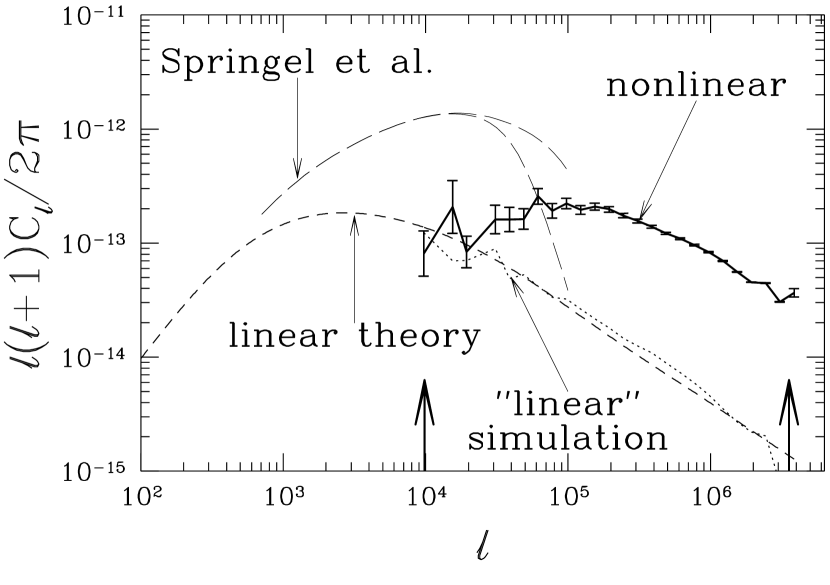
Figure 6: The spectrum of the CMB temperature anisotropy as calculated in linear theory (short-dashed line), from the full numerical simulation (bold solid line), and from the “linear” simulation (dotted line). Also shown with the long-dashed lines the nonlinear power spectra (for two box sizes) of kinetic SZ effect on large scales from Springel et al. (2000).

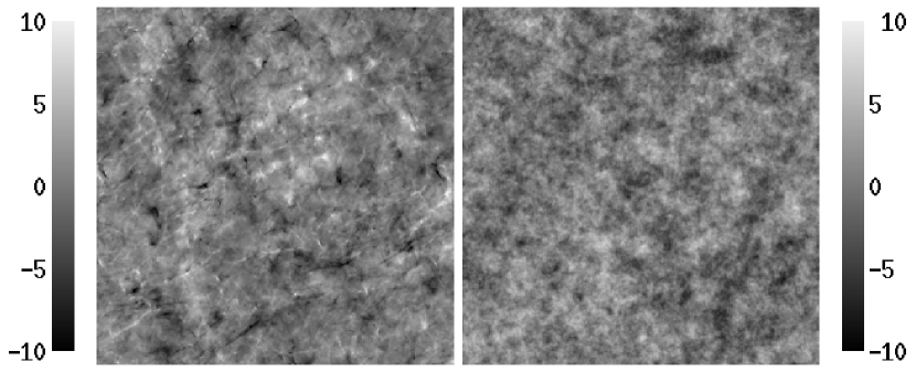
Figure 7: Secondary temperature anisotropies in a $2.2^{\prime}\times 2.2^{\prime}$ patch on the sky as generated during reionization (left panel) and with randomized phases (i.e., a realization of a Gaussian with the same power spectrum, right panel). The color bars show the color-scale correspondence, where the anisotropies are measured in $\mu K$.

The full nonlinear power spectrum is shown with the bold solid line in Fig. 6. In addition, we show the output from our linear “simulation” along with the analytic OV calculation, which match over all scales computed. We emphasize that this agreement requires the imposition of appropriate velocities on scales larger than the simulation box, as discussed above. We also note that our full nonlinear prediction (bold solid line) matches the linear theory on the angular scale corresponding to the box size. This is of course is an artifact of our procedure (and the limited size of our simulation box), which does not include nonlinear perturbations outside the simulation box. In reality, there exists additional power on scales which we can not resolve, simply because the nonlinear scale at $z=0$ is about twice larger than our whole box. To account for this power, we show the nonlinear power spectrum computed by Springel et al. (2000). They assumed precisely the same cosmological model and the redshift of reionization. In addition, their mass resolution almost exactly corresponds to 1/8 of the total mass of our simulation box (corresponding to 1/2 the box size - the largest scale which can be resolved in our simulation). Thus, Springel et al. (2000) begin precisely at the scale where our calculation ends, and we will use their results to compliment ours below. (Conversely, this means that we unfortunately cannot actually check the calculations against one another.)

4 Results

4.1 Maps and non-Gaussianity

It is customary to characterize the CMB temperature anisotropies on the sky by the power spectrum $C_{\ell}$. The power spectrum is sufficient to fully describe properties of a physical quantity only if this quantity is Gaussian distributed. For the primary temperature anisotropies this is indeed the case, since they are generated in the linear regime. Reionization however is a non-linear process, and secondary anisotropies we consider in this paper are not necessarily Gaussian.

This is illustrated in Figure 7, which shows the actual maps of the CMB anisotropies on the square patch on the sky in the simulation. The left panel shows the actual anisotropies on 2.2 arcmin patch on the sky (the angular size of our computational box at $z=8$, just before the full overlap of Hii regions). The right panel, however, shows anisotropies with the same power spectrum but distributed as a Gaussian. We notice that the actual map is highly non-Gaussian: it is much more structured than the Gaussian version and contains higher fluctuations than would be expected in a Gaussian field.

Figure 8: One-point probability distribution of the temperature anisotropies (solid line), the one-point probability distribution of spherical multipole amplitudes $a_{\ell m}$ (dashed line), and a Gaussian distribution (dotted line), all normalized to unit dispersion.

Figure 9: The electron density correlation function $C_{ee}(\eta,\eta+\Delta\eta,\theta)$ as a function of angular size $\theta$ (measured in units of comoving distance $R_{\theta}$ at this redshift) and $\Delta\eta$ (also measured in units of comoving distance $R_{\eta}$) at three redshifts (values of $\eta$): (a) $z=10$, (b) $z=7$, and (c) $z=5$. Subsequently heavier shaded contours show increase in the correlation function by a factor of 10. The outmost contour corresponds to $C_{ee}=1$.

To illustrate this further, we show in Figure 8 the one-point distribution of the actual temperature fluctuations, and a Gaussian distribution for comparison. We notice that the temperature anisotropies are non-Gaussian, and thus more information than simply $C_{\ell}$ can be extracted from the actual distribution on the sky. In addition to temperature anisotropies on the sky, we also show in Fig. 8 the one-point distribution function of spherical multipole amplitudes $a_{\ell m}$, which are defined in the usual fashion by expansion over spherical harmonics,

$${\Delta T\over T}(\theta,\phi)=\sum_{\ell,m}a_{\ell m}Y^{m}_{\ell}(\theta,\phi).$$

The one-point distribution of the amplitudes is actually quite similar to a Gaussian, which indicates that it is indeed the the phase correlations between different multipoles what drive the non-Gaussian patterns. In order to characterize this non-Gaussianity, one would have to measure the higher-order moments (bispectrum, trispectrum, etc.) at non-zero lags, or other quantities such as the Minkowski functionals, but that is outside the scope of this paper.

4.2 Correlation Functions

We now investigate the behavior of the correlation functions. In particular, the electron density correlation function $C_{ee}(\eta_{1},\eta_{2},\theta)$ is of highest interest. We show in Figure 9 the electron density correlation function at three redshifts: before the overlap of Hii regions at $z=10$, during the overlap at $z=7$, and after the overlap at $z=5$. One can notice that there is no drastic change in the shape of the correlation function despite the qualitative change in the structure of the ionized regions; only the correlation length increases with time. This indicates that the signal is dominated by the ionized high density regions at all times, and is not sensitive to the ionization state of the low density intergalactic medium. We will elaborate on this below.

Figure 10: The electron density correlation function $C_{ee}(\eta,\eta,\theta)$ (solid line) and the velocity correlation function $C_{vv}(\eta,\eta,\theta)$ (dashed line) at $z=7$. The dotted line shows the quantity $C_{ev}^{2}/C_{vv}$.

Figure 10 shows both the electron density correlation function $C_{ee}$ and the velocity correlation function $C_{vv}$ as a function of angle (measured as comoving distance at this redshift) at $z=7$. We also show with the dotted line the quantity $C_{ev}^{2}/C_{vv}$, which is much smaller than $C_{ee}$ if the cross-correlation between the electron density and velocity is not significant, and is equal to $C_{ee}$ is they are completely correlated. One can see that the cross-correlation only becomes significant on very small scales, about 0.1 arcsec ($\ell\sim 6\times 10^{6}$), and thus the usual assumption that velocity and electron density are uncorrelated is highly accurate on all scales of interest.

4.3 Kinetic vs Thermal SZ Effect

Figure 11: Comparison of the power spectrum of the secondary CMB anisotropies in the computational box generated by the kinetic SZ effect (eq. [1], solid line) and the thermal SZ effect (eq. [3], dashed line).

It is interesting to compare the kinetic SZ effect given by equation (1) with the thermal SZ effect, given by equation (3). One can expect a priori that the kinetic SZ effect, generated in the gas moving with some $300\mbox{\,km}/\mbox{\,s}$ is about 1000 times more important (in terms of the power spectrum) than the thermal SZ effect, generated due to thermal motions in the $10^{4}\mbox{\,K}$ hot gas. Indeed, this is demonstrated in Figure 11. Thus, for all practical purposes, the kinetic effect is the only one that needs to be taken into account on these scales. Of course, for clusters of galaxies, the situation is reversed and the temperature fluctuation induced by even the several-hundred km/s bulk motion of the cluster is dwarfed by the thermal effect, simply because the cluster gas temperature is some four orders of magnitude higher than the IGM temperature, whereas the bulk gas velocity in a cluster is only about a few times that of the IGM. We return to the comparison between the two effects below.

4.4 The Ostriker-Vishniac Effect versus Patchy Reionization

Figure 12: The electron density correlation function $C_{ee}(\eta,\eta,\theta)$ for the patchy reionization effect ($C_{ee}^{PR}$, solid line) and for the NL Ostriker-Vishniac effect ($C_{ee}^{OV}$, bold dashed line) at $z=9$ (at other redshifts the two correlation functions look quite similar except for the change of the characteristic scale). We also show with the dotted line the quantity $\left(C_{ee}^{OV-PR}\right)^{2}/C_{ee}^{OV}$, which coincides with $C_{ee}^{PR}$ if cross-correlations are important. The thin dotted line shows the NL Ostriker-Vishniac correlation function $C_{ee}^{OV}$ rescaled by the quantity $\left[(1-\bar{x}_{e})/\bar{x}_{e}\right]^{2}$.

We now focus on a comparison between the NL Ostriker-Vishniac effect and patchy reionization. Figure 12 shows the comparison between the two correlation functions $C_{ee}^{PR}$ and $C_{ee}^{OV}$, which are defined by equations (2.2). The dotted line, marking the cross-correlation term in comparison with $C_{ee}^{PR}$, only falls significantly below $C_{ee}^{PR}$ at large radii ($R>0.1h^{-1}\mbox{\,Mpc}$, where the inhomogeneous distribution of the ionized fraction due to expanding Hii regions make the NL Ostriker-Vishniac effect and patchy reionization effect uncorrelated. However, as the thin dashed line shows, in the high density regions (i.e., on small scales) the effect of patchy reionization is almost equivalent to having $x_{e}=1$, i.e., to having almost all high density regions ionized. This implies that the bulk of the signal comes from high density regions and correlations between them.

In order to investigate the relationship between the two effects further, we have constructed a simulation which contains only the “Ostriker-Vishniac” effect by assigning a uniform ionization fraction (equal to the volume average at a given redshift) to the outputs of our full numerical simulation, and performing line-of-sight integration as described above. Thus, this “NLOV simulation” has the density and velocity structure of our full numerical simulation, and has the same evolution of the volume averaged ionization fraction, but has uniform ionization at all densities and spatial locations. In particular, the Patchy Reionization correlation function $C_{ee}^{PR}$ is equal to zero in that simulation, and its NL Ostriker-Vishniac correlation function ($C_{ee}^{OV}$) is the same as in the full simulation. Thus, the NLOV simulation allows us to construct an image of the CMB anisotropies which correspond to just the $C_{ee}^{OV}$ correlation function, whereas the full simulations gives us anisotropies corresponding to the sum of the NL Ostriker-Vishniac and Patchy Reionization effects.

Figure 13: The rms CMB temperature anisotropy as a function of the final redshift of integration for the NL Ostriker-Vishniac effect (dashed line), the patchy reionization effect (dotted line), and for the total effect (the sum of the two, solid line).

Figure 13 now shows the rms temperature anisotropy on the sky (for the $256^{2}$ pixelization) for the total effect, and separately for the NL Ostriker-Vishniac effect (as computed from the “NLOV simulation”) and for the patchy reionization effect (computed as the difference between the two). Note, that by $z=4$ almost all the signal comes from the NL Ostriker-Vishniac effect, and the contribution of the patchy reionization actually slightly declines at $z<7$, after the overlap of Hii regions. This is due to the fact that after the overlap the topology of the ionized phase flips over: reionization starts with isolated ionized regions expanding into the neutral medium, and ends with the isolated neutral regions being ionized from outside inward, which produces an anti-correlation between the ionized and neutral phases and leads to suppression of anisotropies due to patchy reionization.

Figure 14: The solid line shows the total kinetic SZ power spectrum of the secondary CMB anisotropies, computed by combining our full nonlinear results (the solid line from Fig. 6) for $\ell>10^{4}$ with the results of Springel et al. (2000) for $10^{2}<\ell<3\times 10^{4}$ and linear theory for $\ell<10^{2}$), whereas the long-dashed line shows the same calculation for the thermal SZ effect. For both the kinetic and thermal effects, the bold portions of the lines show the regions of the spectrum reliably calculated in this work (large $\ell$ tail), in Springel et al. (2000), or in linear theory, and the thin line shows the regions of $\ell$ where existing predictions are unreliable (and thus the curves we show are somewhat arbitrary). Two dotted lines show the result for the patchy reionization, calculated from our simulation as the difference between the full simulation and the “NLOV simulation” (bold dotted line), and an approximate prediction from Gruzinov & Hu (1998) (thin dotted line). Also shown is the spectrum of primary anisotropies for the assumed cosmological model (thin solid line).

Figure 14 presents now the main result of this paper: the power spectrum of the secondary CMB anisotropies from the kinetic SZ effect, from the thermal SZ effect, and from the patchy reionization effect. For the former two, we combined our results with the calculations by Springel et al. (2000). In the range $3\times 10^{4}\leq\ell\leq 2\times 10^{5}$ our calculation for the kinetic SZ effect disagrees with the extrapolation from the Springel at al. (2000), and for the thermal SZ effect the range of disagreement is even larger. Since our results can suffer from the missing large-scale power at low redshift, and small scale extrapolation of Springel et al. (2000) is likely to be severely affected by limited numerical resolution, it is impossible to give a reliable prediction for the CMB power spectra in this range of angular scales, and we emphasize this fact by using the bold lines to show the calculations where they are reliable, and by using the thin lines in the range of scales where consider calculations to be unreliable.

We also show the prediction from an analytical calculation of the patchy reionization effect by Gruzinov & Hu (1998) for our cosmological model. Note that this prediction is a factor of $10^{2}$ lower than the one given in Gruzinov & Hu (1998) for the standard CDM model, because they adopted the value for the rms velocity at $z=0$ of $1200\mbox{\,km}/\mbox{\,s}$, whereas in our model this number is about 3 times smaller, in agreement with observations (Baker, Davis, & Lin 2000). There is an additional reduction in the amplitude of the effect by a factor of 10 due to the redshift of reionization being 7 in our simulation compared to an adopted value of 30 in Gruzinov & Hu (1998). Including all the relevant factors, we notice that Gruzinov & Hu (1998) estimate gives roughly the right prediction for the patchy reionization effect on large scales. Of course, since the analytical estimate of Gruzinov & Hu (1998) does not include the density structure on small scales, they are unable to reproduce the anisotropies on small angular scales.

4.5 Dependence on the Redshift of Reionization

Up to know we assumed a fixed value for the redshift of reionization, since we only used one simulation. In order to investigate the dependence of the power spectrum on the redshift of reionization properly, we would need to run several simulation with different reionization histories, which is not realistic at the current moment due to required computational resources. However, in order to illustrate the dependence of anisotropies on the redshift of reionization, and using the fact that at $z_{\rm REI}=7$ the NL Ostriker-Vishniac dominates the contribution to the anisotropies due to Patchy Reionization, we have computed three additional “NLOV” simulations where we changed the redshift of reionization by simply rescaling the volume averaged ionization fraction as a function of redshift. In other words, if $n_{e,0}(a)$ is the electron density and $\bar{x}_{e}(a)$ is the volume averaged ionization fraction as a function of the scale factor for the original “NLOV” simulation, for rescaled “NLOV” simulations we assumed

$$n_{e}(a)={\bar{x}_{e}(8a_{\rm REI}a)\over\bar{x}_{e}(a)}n_{e,0}(a),$$

where the factor 8 is simply $1/0.125=1/a_{\rm REI}=1+z_{\rm REI}$ for our simulation.

Figure 15: The power spectra of the secondary CMB anisotropies computed in the “NLOV” simulation with four different values for the redshift of reionization: $z_{\rm REI}=5$ (dotted line), $z_{\rm REI}=7$ (short-dashed line), $z_{\rm REI}=11$ (long-dashed line), and $z_{\rm REI}=19$ (solid line).

Figure 15 shows the CMB power spectra for four different values for the redshift of reionization in our rescaled “NLOV” simulations. We note that in linear theory, $\delta\sim a$ and $v\sim a^{1/2}$ at high redshift, and therefore the total anisotropy

$${\Delta T\over T}\sim\int^{t}a^{3/2}\bar{n}_{b}dt\sim\log(t)$$

goes only logarithmically as a function of the moment of reionization (which is the upper limit in the integral [1] for a model with sudden reionization). The dependence that we find in the nonlinear calculation is somewhat steeper than that from the linear theory, but not by much.

We also note here that the analytical model of patchy reionization by Gruzinov & Hu (1998) predicts that the spectrum of the CMB anisotropies increases as $(1+z_{\rm REI})^{3/2}R_{\mbox{\rm H\sc ii}}$, where $R_{\mbox{\rm H\sc ii}}$ is the characteristic comoving size of Hii regions, which is likely to go down as the redshift of reionization increases. Thus, the total dependence on the redshift of reionization of the patchy reionization effect is somewhat slower than $(1+z_{\rm REI})^{3/2}$ but perhaps not as slow as the nearly logarithmic dependence of the NL Ostriker-Vishniac effect. Thus, if reionization occurred early, the role of patchy reionization (as compared to the NL Ostriker-Vishniac effect) would be greater, albeit the current observational limits of $z_{\rm REI}\lesssim 30$ will not allow a regime when patchy reionization becomes dominant.

5 Conclusions

We use a cosmological numerical simulation that models time-dependent and spatially-inhomogeneous cosmological reionization to compute secondary CMB temperature anisotropies in a representative CDM+$\Lambda$ cosmology. We compare our numerical results with analytical calculations and compliment them with the numerical simulations of Springel et al. (2000) (whose mass resolution almost exactly compliments ours, and accidentally both simulations have the same values of cosmological parameters). We thus are able to compute the power spectrum of secondary anisotropies for the kinetic SZ effect and for the patchy reionization effect over a wide range of angular scales. The thermal SZ effect, dominated at medium $\ell$ by massive clusters of galaxies, is more difficult to compute on all scales due to the extreme non-linearity of the problem.

We find that the role of patchy reionization per se (i.e., evolution of Hii regions around the sources of ionization) in generating the secondary anisotropies is subdominant. This conclusion is however only valid when the sources of reionization are clustered on scales comparable to the matter correlation length, in which case one can expect to find a source (or multiple sources) in almost every dark matter halo. If, in the opposite case, the sources of reionization are rare (like bright quasars), the relative role of patchy reionization will be greater, as many high density regions will remain neutral for a long time, and may not be negligible. The latter scenario is, however, less likely given the current observational limits on the abundances of bright quasars (Fan et al. 2000b), and thus CMB observations on small angular scales may not be as useful as hoped to study the details of reionization.

A real window onto reionization is provided by the detailed morphology of the fluctuations, that is, the non-Gaussianity discussed above. The angular scale of the fluctuations traces the three-dimensional separation scale of the ionized regions. Of course, a full understanding of this will require not just a detection of broad-band fluctuation power at very small angular scales, but a detailed, high signal-to-noise map of these very small-scale fluctuations with an angular resolution of arc seconds, which is definitely some years away.

While the details of reionization may not be easily discernible from the broad-band power spectrum, the amplitude of the fluctuations, which is directly related to the redshift of reionization, surely is. However, as our comparison with Springel et al. (2000) shows, on medium angular scales ($l\lesssim 10^{5}$) the signal is dominated by lower redshifts ($z\sim 2-4$), and only on small angular scales (several arc seconds) the amplitude of the anisotropies is related to the redshift of reionization. In addition, this dependence is quite weak, unless reionization occurred close to the currently allowed observational limit of $z_{\rm REI}\lesssim 30$. Nevertheless, observations on those angular scales can put significant constraints on the redshift of reionization. Such arcsecond-scale CMB observations are best accomplished with interferometers, and indeed the recent development of compact submillimeter-wave arrays has paved the way for such observations. For example, the ATCA telescope finds a limit of $\langle\ell(\ell+1)C_{\ell}/(2\pi)\rangle<2\times 10^{-10}$ at $\ell\sim 4000$ (Subrahmanyan et al. 2000), well above the values presented here. In addition, these observations are inevitably plagued by point source confusion, especially dangerous when the signal also has a compact galaxy-like component.

References

- (1)
- (2) Aghanim, N., Desert, F. X., Puget, J. L., & Gispert, R. 1996, å, 311, 1
- (3)
- (4) Baker, J. E., Davis, M., & Lin, H. 2000, ApJ, submitted (astro-ph/9909030)
- (5)
- (6) Bond, J. R., & Jaffe, A. H. 1999, Phil. Trans. Royal Soc. Lon. A, 357, 57
- (7)
- (8) Benson, A. J., Nusser, A., Sugiyama, N., Lacey, C. G. 2000, MNRAS, in press (astro-ph/0002457)
- (9)
- (10) Bridle, S. L., et al., 1999, MNRAS, 310, 565
- (11)
- (12) Bridle, S. L., Zehavi, I., Dekel. A., Lahav, O., Hobson, M. P., & Lasenby, A. N. 2000, MNRAS, submitted (astro-ph/0006170)
- (13)
- (14) Bruscoli, M., Ferrara, A., Fabbri, R., & Ciardi, B. 2000, MNRAS, submitted (astro-ph/9911467)
- (15)
- (16) de Bernardis, P., et al. 2000, Nature, 404, 955
- (17)
- (18) Eke, V. R., Cole, S., & Frenk, C. S. 1996, MNRAS, 282, 263
- (19)
- (20) Fan, X., et al. 2000a, AJ, submitted (astro-ph/0005414)
- (21)
- (22) Fan, X., et al. 2000b, AJ, submitted (astro-ph/0008123)
- (23)
- (24) Fardal, M.A., Giroux, M.L., & Shull, J.M. 1998, AJ, 115, 2206.
- (25)
- (26) Gnedin, N. Y. 2000, ApJ, 535, 530
- (27)
- (28) Griffiths, L. M., Barbosa, D., Liddle, A. D. 1998, MNRAS, 308, 854
- (29)
- (30) Gruzinov, A., & Hu, W. 1998, ApJ, 508, 435
- (31)
- (32) Haiman, Z., & Knox, L. 1999, in ASP Conf. Ser. 181, Microwave Foregrounds, ed. A. de Oliveira-Costa & M. Tegmark (San Francisco: ASP), 227
- (33)
- (34) Hanany, S., et al. 2000, ApJ, submitted (astro-ph/0005123)
- (35)
- (36) Hu, W. 2000, ApJ, 529, 12
- (37)
- (38) Hu, W., Fukugita, M., Zaldarriaga, M., & Tegmark, M. 2000, ApJ, submitted (astro-ph/0006436)
- (39)
- (40) Hu, W., & White, M. 1996, å, 315, 33
- (41)
- (42) Jaffe, A. H., & Kamionkowski, M. 1998, Phys. Rev. D, 58, 043001
- (43)
- (44) Jaffe, A. H., et al. 2000, Phys. Rev. Lett., submitted (astro-ph/0007333)
- (45)
- (46) Knox, L., Scoccimarro, R., & Dodelson, S. 1998, Phys. Rev. Lett., 81, 2004
- (47)
- (48) Melott, A. L. 1994, ApJ, 426, L19
- (49)
- (50) Ostriker, J. P, & Vishniac, E. 1986, ApJ, 306, 51
- (51)
- (52) Peebles, P. J. E., & Juszkiewicz, R. 1998, ApJ, 509, 483
- (53)
- (54) Refregier, A., Komatsu, E., Spergel, D. N., & Pen, U.-L. 2000, Phys. Rev. D, in press (astro-ph/9912180)
- (55)
- (56) Seljak, U., Burwell, J., & Pen, U.-L. 2000, Phys. Rev. D, submitted (astro-ph/0001120)
- (57)
- (58) da Silva, A. C., Barbosa, D., Liddle, A. R., & Thomas, P. A. 2000, MNRAS, in press (astro-ph/9907224)
- (59)
- (60) Springel, V., White, M., & Hernquist, L. 2000, ApJ, submitted (astro-ph/0008133)
- (61)
- (62) Stern, D., et al. 2000, ApJ, 533, L75
- (63)
- (64) Subrahmanyan, R., Kesteven, M. J., Ekers, R. D., Sinclair, M.,Silk, J., MNRAS, to appear. astro-ph/0002467
- (65)
- (66) Tegmark, M., Zaldarriaga, M. 2000, Phys. Rev. Lett., in press (astro-ph/0004393)
- (67)
- (68) White, M., Scott, D., & Pierpaoli, E. 2000, ApJ, in press (astro-ph/0004385)
- (69)
- (70) Zheng, W., et al. 2000, AJ, submitted (astro-ph/0005247)
- (71)