Snapshot Identification of Gamma Ray Burst Optical Afterglows

Abstract

Gamma ray burst afterglows can be identified in single epoch observations using three or more optical filters. This method relies on color measurements to distinguish the power law spectrum of an afterglow from the curved spectra of stars. Observations in a fourth filter will further distinguish between afterglows and most galaxies up to redshifts $z\approx 1$. Many afterglows can also be identified with fewer filters using ultraviolet excess, infrared excess, or Lyman break techniques. By allowing faster identification of gamma ray burst afterglows, these color methods will increase the fraction of bursts for which optical spectroscopy and other narrow-field observations can be obtained. Because quasar colors can match those of afterglows, the maximum error box size where an unambiguous identification can be expected is set by the flux limit of the afterglow search and the quasar number-flux relation. For currently typical error boxes (10 – 100 square arcminutes), little contamination is expected at magnitudes $R\lesssim 21.5\pm 0.5$. Archival data demonstrates that the afterglow of GRB 000301C could have been identified using this method. In addition to finding gamma ray burst counterparts, this method will have applications in “orphan afterglow” searches used to constrain gamma ray burst collimation.

1 Introduction

The search for counterparts to gamma ray bursts (GRBs) at longer wavelengths has been recognized from the beginning as a key to understanding the bursts’ nature. This motivated models that predicted gamma ray burst afterglows from hot material in relativistically expanding GRB remnants (Paczyński & Rhoads 1993; Katz 1994; Mészáros & Rees 1997). The afterglow was predicted to arise from synchrotron radiation, and its spectrum is therefore well described by a broken power law. Both the prediction of fading counterparts with power law spectra and the general expectation that GRB counterparts would tell us a great deal about the bursts have been amply borne out by observation since the first successful observations of GRB afterglows in 1997 (Costa et al 1997; van Paradijs et al 1997; Frail et al 1997).

The greatest rewards so far have come from detailed studies of individual afterglows with the best time and spectral coverage. Rapid afterglow identifications are a key to achieving such data sets, because some essential types of data cannot be obtained before the afterglow position is known to $\sim 1$ arcminute (near-infrared and submillimeter photometry) or even $\sim 1$ arcsecond (spectroscopy). Traditionally, afterglows are found through a variability search within GRB error boxes. This requires multiple epoch observations whose separation in time $\Delta t$ must be a reasonable fraction ($\gtrsim 0.3$) of the time elapsed from the GRB to the first epoch. This lag is usually further increased by telescope scheduling issues to $\sim 1$ day. Moreover, afterglow light curves occasionally include “plateau” phases (e.g. GRB 970508 at $t<2$ days [Pedersen et al 1998]; GRB 971214 at $t<0.3$ days [Gorosabel et al 1998]; and GRB 000301C at $t\sim 6$ days [Bernabei et al 2000; Masetti et al 2000]). Two-epoch observations of such afterglows could miss them entirely.

This delay in afterglow identification is not necessary, because afterglows are characterized not only by fading behavior but also by power law spectra. Such spectra are relatively rare in the optical sky, which is dominated by Galactic stars at bright flux levels and by galaxies at faint flux levels. Relative to a stellar spectrum, a GRB afterglow is blue at blue wavelengths ($\lesssim 0.4\mu m$), and red at red wavelengths ($\gtrsim 0.6\mu m$). A color-color plot should therefore isolate a GRB afterglow from nearby stars efficiently, provided it spans a sufficient wavelength range to detect spectral curvature (or the Balmer jump) in stars of any surface temperature. Under many circumstances it will also be possible to identify afterglows using simpler though less robust single color criteria (either ultraviolet excess [“UVX”] or infrared excess [“IRX”]). Moreover, absolute photometric calibration is not required so long as a sufficient solid angle is observed to empirically determine the stellar locus in color space.

Section 2 describes model color-color plots that show the expected loci of GRB afterglows, stars, galaxies, and quasars. Section 3 demonstrates empirically that the color-color method could have identified the afterglow of GRB 000301C in a single epoch. Finally, section 4 considers advantages and limitations of the method, including confusion limits as a function of flux level, likely selection effects in the sample of afterglows found through color-based searches, and applicability of the method to “orphan afterglow” searches.

2 Color-Color Space Models

To explore this method in detail, I have calculated synthetic color space locations for GRB afterglows, stars, galaxies, and quasars. Model calculations were performed for the widely available Johnson U, B, and V filters and Cousins R and I filters, though color-color searches will work for any set of filters spanning a sufficient wavelength range. Filter transmission curves were taken from Bessell (1990). The photometric zero point for all Johnson-Cousins system synthetic colors was set to the Vega model atmosphere of Kurucz (1979).

Model spectra of objects at high redshift were attenuated using the mean intergalactic absorption given by Madau (1995). For redshifts $z\gtrsim 2$, the flux in the bluest filter can be greatly reduced by neutral hydrogen absorption in the intergalactic medium. This absorption consists of a superposition of Lyman $\alpha$ forest lines, higher order Lyman lines, and bound-free Lyman continuum absorption (Madau 1995). The net effect is a shift in the bluest color measured. The relevant redshift depends on the choice of bluest filter. The Lyman $\alpha$ line is redshifted to the peak transmission wavelength of the Johnson U band at $z=2.04$, and the Johnson B filter around $z=2.5$.

In addition, I calculated reddening vectors for dust both in the Milky Way and in afterglow host galaxies at a range of redshifts, using the empirical fits of Pei (1992) to the extinction laws of the Milky Way and the Magellanic Clouds.

In the following subsections, I describe the color calculations for each class of object considered, and then summarize the results.

Stars:

Stellar colors were derived from the spectrophotometric catalog of Gunn and Stryker (1983), which spans spectral types from O to M and luminosity classes from the main sequence to supergiants.

GRB Afterglows:

Afterglows were taken as pure power law spectra, $f_{\nu}\propto\nu^{\alpha}$, with indices $0.5\lesssim-\alpha\lesssim 1.5$. Such spectra describe synchrotron emission from a power law distribution of electrons away from break frequencies. Deviations from power law spectra occur near spectral breaks (see Sari, Piran, & Narayan 1998) and in the case of interstellar absorption (section 4). The range of spectral indices considered corresponds to the commonly measured range of electron energy indices, $2<p<3$. Here $p$ describes the number-energy distribution of electrons accelerated at the GRB remnant’s external shock, $N({\cal E})\propto{\cal E}^{-p}$, and I have considered spectra both above and below the cooling frequency.

Galaxies:

Galaxy spectra were taken from the GISSEL stellar population synthesis code (Bruzual & Charlot 1993) for a few representative star formation histories. No attempt was made to include galaxy evolution effects, which may result in elliptical galaxy colors that are slightly too red at high redshift (see, e.g., Bruzual [1996]). The resulting galaxy colors agree with those computed by Fukugita, Shimasaku, & Ichikawa (1995) to within $0.1\,\hbox{mag}$ for most filters, galaxy spectral types, and redshifts; this is acceptable given the differences in the input spectra in the two works.

Galaxy spectra at optical wavelengths are a superposition of diverse stellar spectra, modified slightly by nebular emission and dust effects. This superposition implies that galaxies have less sharply peaked spectra than individual stars and so lie on the same side of the color-color space stellar locus as power law spectra. Indeed, the spectrum of a star forming galaxy can be a good power law over most of the optical window. Fortunately, the $4000$Å break due to stellar atmospheric features interrupts this approximate power law and can be used to distinguish almost all galaxies at $z\lesssim 1$ from afterglow candidates given sufficient color information. With observations in three filters, there is some redshift where the $4000$Å break lies in the middle filter, and galaxy colors can match those of a pure power law. The addition of a fourth filter breaks this degeneracy. For example, in the $U-B$, $R-I$ plane, an irregular galaxy at $z\approx 0.4$ lies on the power law sequence; however, its $B-R$ color is much redder than the corresponding power law. In addition to color criteria, it is of course possible to distinguish galaxies from GRB afterglows morphologically. The fraction of galaxies that appear extended depends on the available spatial resolution, with the a few galaxies appearing pointlike even in Hubble Space Telescope images, but subarcsecond resolution will in practice greatly reduce confusion due to galaxies.

Quasars:

Quasar colors were calculated using the composite quasar spectrum by Francis et al (1991), extrapolated to $\lambda>0.6\mu m$ with $f_{\lambda}\propto\lambda^{-2.18}$. This extrapolation will result in modest color errors for low redshifts where the H$\alpha$ line falls in a measured filter, but should not affect our conclusions greatly.

Quasar spectra are reasonably well approximated by power laws (plus broad emission lines) across a wide wavelength range. Color-based criteria have been used to identify quasars for nearly 40 years (see the review by Burbidge 1967), and the use of far-red filters to supplement bluer UBV passbands was suggested as early as 1967 (Braccesi 1967; Braccesi, Lynds, & Sandage 1968). Quasars are therefore extremely difficult to distinguish from GRB afterglows using only broad band colors. The main discriminant available is that quasars tend to be somewhat bluer than typical afterglows. In practice, we expect confusion with quasars to set the maximum area over which an unambiguous afterglow identification can be expected. This confusion can be resolved with low resolution spectra, which identify most quasars unambiguously by their strong, broad emission lines.

2.1 Results

Sample color-color diagrams are shown for the $U-V$, $V-I$ plane in figure 1, and the $B-V$, $R-I$ plane in figure 2. These have been chosen as representative cases where the two-color method works. Additional combinations of filters are also effective provided that at least three filters are used, the bluest filter is at least as blue as the Johnson B band, and the reddest is at least as red as Cousins I. Unfortunately, the observationally easiest filters (BVR) do not yield an adequate separation between afterglow and stellar colors to expect reliable identification of afterglows, barring unusually high photometric precision.

Figure 1: Model U-V, V-I color-color plane. 5-pointed stars mark the location of GRB afterglows, represented by pure power law spectra with indices $f_{\nu}\propto\nu^{\alpha}$ for $\alpha=-0.5,-1.0,-1.5$. Small points represent stars from the Gunn-Stryker (1983) atlas. Dotted lines show the locations of different galaxy spectra as a function of redshift. Star formation activity increases from lower right (Elliptical galaxy model) through spiral models (Sb and Sc) to an actively star forming Magellanic irregular (Im) model. Open circles along these tracks mark intervals of 0.5 in redshift, from zero to 3.0. No galaxy evolution is incorporated in these tracks. Finally, the solid line shows the locus of quasars as a function of redshift. Filled points along this track again mark redshift intervals of 0.5 from zero to 3.0. Intergalactic absorption will shift the afterglow locus to redder $U-V$ at fixed $V-I$ for $z\gtrsim 2.0$.

Figure 2: Model B-V, R-I color-color plane. Symbols are the same as for figure 1. Because neutral hydrogen absorption first becomes important at higher redshift in the B band than the U band, color tracks for galaxies and quasars extend to somewhat higher redshift here, and the afterglow locus shifts to redder $B-V$ for $z\gtrsim 2.5$.

Given a sufficient filter set, the afterglows are well separated from the stellar locus. Moreover, the reddening vector for Milky Way dust runs essentially parallel to both the stellar sequence and the power law spectral sequence. Thus, even though reddened afterglow spectra are no longer strict power laws, they remain distinct in color-color space.

Of greater concern is dust in the GRB host galaxy. Because this dust is at high redshift, its $2175$Å feature can enter the observed wavelength range, changing the direction of the reddening vector in color-color space. For redshifts $2.2\lesssim z\lesssim 3.3$, this feature falls in the reddest filter of the color-color plot, thus making the long-wavelength color (e.g., V-I) slightly bluer. A moderate amount of dust ($A_{V}=0.5$) can then move the afterglow locus onto the stellar locus in color-color space. However, this effect is only important for Milky-Way type dust. The most important consequence of dust for color-based afterglow searches is therefore not reddening but extinction, which can reduce the received flux below the detection limit of the search whatever the reddening law. However, GRBs can destroy dust at distances up to $10~{}pc$ (Waxman & Draine 2000) or beyond (Fruchter, Krolik, & Rhoads 2001), reducing these concerns substantially for bursts at high Galactic latitude.

3 Empirical Tests

Archival multicolor data is available for a few GRB fields from the U.S. Naval Observatory’s GRB followup team (see Henden et al 2000). I have used this data for the field of GRB 000301C, together with published photometry of the afterglow (Jensen et al 2000), for an empirical demonstration of color-based optical afterglow searches.

Two color-color plots for this field are shown in figure 3. In both cases, we see that the afterglow is an outlier in color-color space. In the $U-V$, $V-I$ figure, there are a few other outliers, all of which are systematically redder than the afterglow in both colors. In the $B-V$, $R-I$ plot, the afterglow is the single most dramatic outlier and would be the first target chosen for prompt spectroscopy or other rapid narrow-field followup observations.

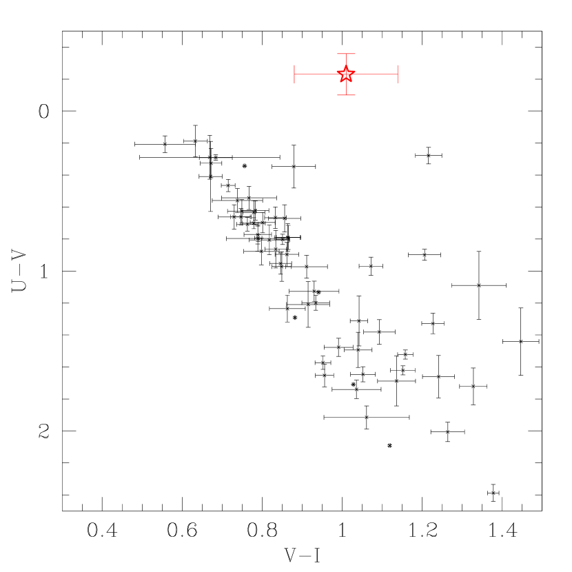
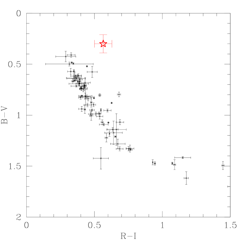
Figure 3: Color-color plots for the field of GRB 000301C. Data are taken from Jensen et al (2000) for the GRB afterglow (marked by a five-pointed star symbol); and from Henden et al (2000) for other objects in the field. For the Henden et al data, error bars on U-V were computed by adding in quadrature the reported U-B and B-V errors; similarly, V-I errors were computed from V-R and R-I. The GRB is an outlier in both plots, and the most dramatic outlier in the B-V, R-I plane.

4 Discussion

Color-based searches have the potential to identify GRB afterglows faster than a two-epoch variability search, and hence to allow more thorough followup of many afterglows. There are three basic color selection criteria available for afterglows: IR excess (“IRX”), UV excess (“UVX”), and Lyman break. The appropriate combination of these depends on both the redshift of the burst and the available instrumentation. The primary focus of this paper is on color-color plane methods, which combine the IR excess and UV excess criteria and are therefore more robust than either criterion alone.

Still, as the observations of GRB 000301C demonstrate, potentially occupied regions of color-color space remain vacant in practice for high-latitude fields observed to a limiting magnitude $V\sim 21$. In particular, there are no very hot stars, few or no high redshift galaxies, and few or no quasars. Under these circumstances, a simple UV Excess (“UVX”) test could identify the afterglow on the basis of a single color measurement (preferably including one filter at $\lambda<4000$Å).

Likewise, at near-infrared wavelengths, most stars and galaxies will have spectral slopes near the Rayleigh-Jeans value ($2$) and will therefore be bluer than afterglows. This is again demonstrated by GRB 000301C, for which we found $J-K^{\prime}\approx 1.45$ (Rhoads & Fruchter 2001), about $0.3$ magnitudes redder than even the coolest stars tabulated by Johnson (1966). However, UVX and IRX methods are vulnerable to the presence of very hot stars and highly reddened sources respectively, while the two color method is not.

The Lyman break (or “dropout”) method uses intergalactic absorption to find high redshift afterglows whose strongly attenuated blue flux places them in a region of color space occupied by essentially all classes of high redshift object, on the opposite side of the stellar locus from low redshift afterglows. The observational requirements to find these bursts from Lyman break colors are more exacting. Long integrations in the bluest filter are required to conclusively identify “dropout” afterglows, while lower redshift afterglows are unusually bright in the bluest filter and require correspondingly shorter integrations. Even so, most afterglows are brighter than their host galaxies at discovery, which means that a high redshift afterglow may be an easier dropout to identify than a high redshift galaxy.

Color-based searches are subject to certain selection effects, which must be considered in interpreting their results. These effects include: (1) Redshift: The onset of intergalactic hydrogen absorption in the bluest filter observed determines the highest redshift where UV excess methods can work and the lowest redshift where Lyman break methods can work. The UVX method will fail at $z\approx 2$ for U band and $z\approx 2.5$ for B band, while the Lyman break method first becomes practical in the U band at $z\approx 3.3$. Thus, two-color optical searches will not identify afterglows between about $z=2.5$ and $z=3.3$. The IR excess will continue to be practical to quite high redshift, e.g. to $z\approx 15$ for a $J-K$ color, since the onset of neutral hydrogen absorption simply accentuates an IR excess until the absorption reaches the redder filter. Because there is considerable variance in the hydrogen column density along different lines of sight (Madau 1995), the redshift boundaries discussed here are not sharp demarcations. Rather, the detection efficiency declines smoothly, and the characteristic redshifts given above correspond to about $50\%$ of peak efficiency.

(2) Heavily obscured afterglows can drop below the search’s detection threshold. Extinction affects any search method, though it is exacerbated for UVX and two-color methods by the increase of extinction towards bluer optical-UV wavelengths and the necessity of observations in observer frame blue light. Additionally, there will be a mild selection against finding afterglows in galaxies with Milky Way type dust extinction at redshifts $2.2\lesssim z\lesssim 3.3$ using two-color optical searches. However, this overlaps the stronger selection due to intergalactic Hydrogen absorption to such an extent as to be almost unimportant.

(3) For gamma ray bursts occurring near dense molecular gas, absorption by excited molecular hydrogen can occur for rest wavelengths as long as $1650$Å (Draine 2000). Absorption between $1650$ and $1300$Å can reach 50% for H₂ column densities around $10^{19}$ cm^-2. This will act to exclude afterglows in molecular clouds from UVX or two-color samples at redshifts beyond $1.3$ (using U band) or $1.65$ (using B).

(4) Because afterglow spectra are broken power laws rather than pure power laws, there will be times in the evolution of each afterglow when its colors deviate from the models in section 2. Breaks in synchrotron spectra are not absolutely sharp, so this is unlikely to be a major selection effect for purely optical searches, where the wavelength range spanned is only a factor of $\sim 2.5$. Searches employing larger wavelength coverage (UV or IR) will be more sensitive to this effect.

(5) Afterglows located atop brighter host galaxies may be hard to find because the dominant color is that of the galaxy. This effect will depend on instrumental spatial resolution as well as the intrinsic properties of the afterglow and host galaxy. (Variability searches can be similarly compromised unless image subtraction methods are used.)

(6) An advantage of this method is that short-term “plateaus” in afterglow light curves do not affect it. It may therefore find some afterglows that traditional variability searches miss.

Even afterglows that lie in the predicted region of color space may be difficult to identify by these methods in cases where the error box is so large that a substantial number of other sources occupy the same region of color space. The critical error box size where one “confusing” source is expected depends on the magnitude limit of the search. Ultimately, the quasar number-flux relation gives a lower limit to the confusion level. Additionally, for three filter searches, star forming galaxies at $z\sim 0.5$ can add to the confusion. To achieve a unique afterglow identification, it is necessary to match the magnitude limit of the search to the size of the error box, and to observe the field while the afterglow remains brighter than this magnitude limit. A unique identification may not always be needed, however. In particular, a list of several viable candidates may be enough to obtain a same-night afterglow spectrum using a multiobject spectrograph with a sufficient field of view and rapid setup procedure. The correct candidate could then be identified later based on either spectra or variability.

The quasar number-magnitude relation for $z<2.2$ and magnitude $B<24$ is predicted by Malhotra & Turner (1995) for both ($\Omega=1$, $\Lambda=0$) and ($\Omega=0.1$, $\Lambda=0.9$) cosmologies, based on observations to $B<22$ by Boyle et al (1987) and Boyle, Shanks, & Peterson (1988).

The approximate range of redshift where star forming galaxies overlap the GRB afterglow locus in color-color space is $0.35\lesssim z\lesssim 0.6$ for the $U-V$, $V-I$ diagram, or $0.45\lesssim z\lesssim 0.6$ for the $B-V$, $R-I$ diagram. I estimate a number-magnitude relation for such galaxies using both the local luminosity function from Loveday et al (1992) and direct counts of galaxies with $0.55<V-I<1.28$ and $0.4<z<0.6$ from the Canada-France Redshift Survey (Lilly et al 1995a; Le Fevre et al 1995; Hammer et al 1995). The predicted number counts amount to approximately 10% of all galaxy number counts (see, e.g., Lilly et al 1995b, Williams et al 1996) around $R=22$. The quasar and galaxy count estimates (converted to R band magnitudes using the colors of an $f_{\nu}\propto\nu^{-1}$ power law) are plotted together in figure 4. We see that quasars are the more important foreground for $R<20$. At fainter magnitudes, galaxies appear more important, but this may be misleading since they can often be identified using a third independent color and/or morphological information.

Figure 4: Cumulative number-magnitude relation for sources whose optical colors resemble GRB afterglows. The solid lines shows quasar counts predicted by models A and B of Malhotra & Turner (1995). The dotted line shows the predicted number counts for galaxies with $0.4<z<0.6$ using the locally derived luminosity function from Loveday et al (1992). Counts of blue galaxies should be $\sim 30\%$ lower. The histogram shows the Canada-France Redshift Survey data for galaxies with $0.4<z<0.6$ and with $V-I$ colors in the afterglow range (Lilly et al 1995a; Le Fevre et al 1995; Hammer et al 1995). The total number of galaxies around 22nd magnitude is a factor $\sim 10$ above the galaxy counts shown. The plotted curves can be taken as an approximate guide to the number of potentially confusing sources expected for a given area searched and limiting magnitude attained. The exact number can depend substantially on additional factors, in particular photometric accuracy, spatial resolution, and the availability of a third independent color to distinguish $z\sim 0.5$ galaxies from afterglows.

Presently, most GRB error boxes have characteristic sizes of a few tens of square arcminutes. Thus, the brightest quasar expected in the error box has a magnitude $R\sim 22$, while the brightest galaxy having colors similar to an afterglow might be a magnitude brighter. Both this depth and the error box area are reasonably well matched to the capabilities of moderate sized (1 to 2.5 meter) ground-based telescopes.

4.1 Optimizing the Observations

To realize the promise of same-night afterglow identifications, a rapid and standard data analysis procedure is desirable, and could be aided by an observing procedure optimized for quick analysis. Archival bias frames and flatfield frames for all filters could be useful, and precisely cospatial exposures in multiple filters (i.e., without offsets and with telescope guiding) could ease measurement of object colors.

An additional constraint on observing strategy arises because the target is likely to fade during the period of observations. If the multiple wavelengths cannot be observed simultaneously, it is then better to begin with the bluest filter, followed by the reddest, and only then move on to the middle filters. This way, fading behavior will accentuate the expected color offset rather than reducing it. (The choice of bluest filter before reddest is driven by the possibility that a spectral break may move through the observed wavelength range during the course of observations.)

The optimal choice of filter set will depend on local conditions. The relative difficulty of U band observations is approximately balanced by the large color-plane offsets obtained with U data ($\sim 0.7~{}\,\hbox{mag}$ from the stellar locus), which relax the signal to noise requirements considerably.

4.2 Orphan Afterglow Searches

If gamma ray bursts are highly collimated, we expect to observe many more afterglows than GRBs (Rhoads 1997). The search for such “orphan afterglows” is an important and largely model-independent way of testing GRB collimation.

Color-based techniques will be a valuable addition to orphan afterglow searches. Afterglows remain rare phenomena even in extreme collimation scenarios, and in order to find one it will be necessary to survey a large area of sky that will contain many quasars. Thus, orphan afterglow searches must combine variability with color tests to be reliable. When enough filters are observed simultaneously in a field where an archival first epoch is available, it will be possible to identify new sources, test their colors for consistency with a power law spectrum, and start intensive followup of any viable afterglow candidates. This will allow much greater confidence in the identification of orphan afterglows than is presently possible, since good spectra and light curves can then be used to distinguish real afterglows from variable stars, high redshift supernovae, active galactic nuclei, microlensing events, and other optically variable sources.

As an illustrative example, consider Sloan Digital Sky Survey (SDSS; see Knapp et al 1999). The SDSS southern strip will cover an area $\sim 200$ degree² to about 22nd magnitude in 5 broadband filters many ($\sim 45$) times. The known GRB rate is $\sim 3$ per sky per day, and bright afterglows remain above 22nd magnitude for a period $\sim 4$ days. Thus the southern strip has an effective coverage of $4\times 10^{4}\hbox{degree}^{2}\,\hbox{day}$. The northern SDSS survey will cover $10^{4}$ degree² in a single imaging epoch. Fortunately, GRB afterglows would likely be targeted for spectra based on their quasar-like colors, yielding a second epoch. The northern survey thus provides another $\sim 4\times 10^{4}\hbox{degree}^{2}\,\hbox{day}$. Both parts together would be expected to detect $\sim 6$ GRB afterglows. If GRBs are tightly collimated (opening angles $\lesssim 10^{\circ}$), the expected number of orphan afterglows rises to $\gtrsim 25$. By using the color space properties to identify these afterglows, such a survey can place strong limits on the collimation angle and hence energy requirements of gamma ray bursts.

5 Conclusions

Color-based searches will allow faster identification of many gamma ray burst afterglows. Intensive followup of these afterglows can then begin earlier and at brighter flux levels, yielding a larger sample of bursts for which spectroscopic redshifts and well measured spectral energy distributions (including roughly synoptic data at X-ray, optical, near-infrared, submillimeter, and radio wavelengths) can be obtained. Such data sets are crucial to detailed studies of afterglow physics. Additionally, single-epoch color-based searches may yield a more easily characterized statistical sample of afterglow detections and nondetections than is currently available. Such samples will allow reliable studies of the population properties of gamma ray burst afterglows, and thereby open the way for new insights into the nature of gamma ray bursts.

References

- (1) Bernabei, S., Bartolini, C., Di Fabrizio, L., Guarnieri, A., Piccioni, A., & Masetti, N. 2000, GCNC 599
- (2) Bessell, M. S. 1990, PASP 102, 1181
- (3) Boyle, B. J., Fong, R., Shanks, T., & Peterson, B. A. 1988, MNRAS 227, 717
- (4) Boyle, B. J., Shanks, T., & Peterson, B. A. 1988, MNRAS 235, 935
- (5) Braccesi, A. 1967, Nuovo Cimento, Ser. 10, 49, 148
- (6) Braccesi, A., Lynds, R., & Sandage, A. 1968, ApJ 152, L105
- (7) Bruzual A., G., & Charlot, S. 1993, ApJ 405, 538
- (8) Bruzual A., G. 1996, in ASP Conference Series 98, From Stars to Galaxies: The Impact of Stellar Physics on Galaxy Evolution, eds. C. Leitherer, U. Fritze-v. Alvensleben, & J. Huchra (San Francisco: ASP), 14
- (9) Burbidge, E. M. 1967, ARA&A 5, 399
- (10) Costa, E., et al 1997, IAU Circular 6572
- (11) Draine, B. T. 2000, ApJ 532, 273
- (12) Frail, D. A., Kulkarni, S. R., Nicastro, L., Feroci, M., & Taylor, G. B. 1997, Nature 389, 261
- (13) Francis, P. J., Hewett, P. C., Foltz, C. B., Chaffee, F. H., Weymann, R. J., & Morris, S. L. 1991, ApJ 373, 465.
- (14) Fruchter, A. S., Krolik, J. H., & Rhoads, J. E. 2001, submitted to ApJ
- (15) Fukugita, M., Shimasaku, K., & Ichikawa, T. 1995, PASP 107, 945
- (16) Gorosabel, J., et al 1998, A&A335, L5
- (17) Gunn, J. E., & Stryker, L. L. 1983, ApJS 52, 121
- (18) Hammer, F., Crampton, D., Le Fevre, O., & Lilly, S. J. 1995, ApJ 455, 88
- (19) Henden, A. A., and the USNO GRB team, GCN Circular 583, 2000
- (20) Jensen, B. L., et al 2000, submitted to A&A; astro-ph/0005609
- (21) Johnson, H. L. 1966, ARA&A 4, 193
- (22) Katz, J. I. 1994, ApJ 422, 248
- (23) Knapp, G. R., Gunn, J. E., Margon, B., Lupton, R. H., York, D., & Strauss, M. 1999, The Sloan Digital Sky Survey Project Book, Version V1.3
- (24) Kurucz, R. L. 1979, ApJS 40, 1
- (25) Le Fevre, O., Crampton, D., Lilly, S. J., Hammer, F., & Tresse, L. 1995, ApJ 455, 60
- (26) Lilly, S. J., Hammer, F., Le Fevre, O., & Crampton, D. 1995a, ApJ 455, 75
- (27) Lilly, S. J., Hammer, F., Le Fevre, O., & Crampton, D. 1995b, ApJ 455, 108
- (28) Loveday, J., Peterson, B. A., Efstathiou, G., & Maddox, S. J. 1992, ApJ 390, 338
- (29) Madau, P. 1995, ApJ 441, 18
- (30) Malhotra, S., & Turner, E. L. 1995, ApJ 445, 553
- (31) Masetti, N., et al 2000, A&A 359, L23
- (32) Mészáros, P., & Rees, M. J. 1997, ApJ 476, 232
- (33) Paczyński, B., & Rhoads, J. E. 1993, ApJ 418, L5
- (34) Pedersen, H., et al 1998, ApJ 496, 311
- (35) Pei, Y. C. 1992, ApJ 395, 130
- (36) Rhoads, J. E. 1997, ApJ 487, 1
- (37) Sari, R., Piran, T., & Narayan, R. 1998, ApJ 497, 17
- (38) van Paradijs, J., et al 1997, Nature 386, 686
- (39) Waxman, E., & Draine, B. T. 2000, ApJ 537, 796
- (40) Williams, R., et al 1996, AJ 112, 1335