The warm circumstellar envelope and wind of the G9 IIb star HR 6902

Abstract

IUE observations of the eclipsing binary system HR 6902 obtained at various epochs spread over four years indicate the presence of warm circumstellar material enveloping the G9 IIb primary. The spectra show Si iv and C iv absorption up to a distance of 3.3 giant radii (${\rm R_{g}}$). Line ratio diagnostics yields an electron temperature of $\rm\sim 78\,000\;K$ which appears to be constant over the observed height range.

Applying a least square fit absorption line analysis we derive column densities as a function of height. We find that the inner envelope ($<3\;{\rm R_{g}}$) of the bright giant is consistent with a hydrostatic density distribution. The derived line broadening velocity of $\sim 70\;{\rm km\,s^{-1}}$ is sufficient to provide turbulent pressure support for the required scale height. However, an improved agreement with observations over the whole height regime including the emission line region is obtained with an outflow model. We demonstrate that the common $\beta$ power-law as well as a $P\propto\rho$ wind yield appropriate fit models. Adopting a continuous mass outflow we obtain a mass-loss rate of $\dot{M}=0.8-3.4\times 10^{-11}$ $\rm M_{\odot}\,{yr^{-1}}$ depending on the particular wind model.

The emission lines observed during total eclipse are attributed mostly to resonance scattering of B star photons in the extended envelope of the giant. By means of a multi-dimensional line formation study we show that the global envelope properties are consistent with the wind models derived from the absorption line analysis. We argue that future high resolution UV spectroscopy will resolve the large-scale velocity structure of the circumstellar shell. As an illustration we present theoretical Si iv and C iv emission profiles showing model-dependent line shifts and asymmetries.

1 Introduction

The spectroscopic binary system HR 6902 (G9 IIb + B8-9 V) belongs to the category of $\zeta$ Aur stars, where a hot companion (generally a main sequence B star) moves through the extended envelope of an evolved late-type star. The specific binary geometry provides an exceptional opportunity to probe the spatial dependence of the physical properties of the outer atmosphere and wind of the primary. Observations of $\zeta$ Aur systems and related objects with the International Ultraviolet Explorer (IUE) and more recently with the Hubble Space Telescope (HST) take advantage of the ultraviolet spectral region. At wavelengths below $\sim 3000\;\mathrm{\AA}$ the hot secondary dominates the observed flux allowing a separation of the spectral information. In the UV the observed spectrum is purely that of the companion with superimposed circumstellar and interstellar lines. Further information on the binary technique can be found in several reviews (e.g., Reimers (1989); Guinan (1990); Ahmad (1993); Harper (1996); Baade (1998)).

Ground based spectroscopic as well as UV and X-ray observations from space of stars in the cool half of the HR diagram have shown that the extended atmospheres of giants and supergiants undergo a dramatic physical change across a region in the HR diagram. To the right of this transition we observe cool and massive winds plus extended cool chromospheres, while to its left there is much hotter circumstellar matter. This transition is accompanied by different spectral indicators defining distinct dividing lines. The leftmost is the ”X-ray dividing line”. All stars to its left show X-ray emission, probably arising from extended corona-like plasma (e.g., Haisch, Schmitt, & Rosso 1991, 1992). In the ultraviolet the same stars also show C iv and Si iv and often N v emission (Linsky & Haisch (1979)). Additional dividing lines are defined by asymmetries in the Ca ii and Mg ii emission lines (e.g., Stencel & Mullan 1980a , 1980b). The strongest and most reliable evidence for the existence of a cool, massive wind is the appearance of circumstellar absorption features in the Ca ii line (Reimers (1977)). A theoretical discussion of the dividing line concept based on hydromagnetic waves can be found in Rosner (1993) and Rosner et al. (1995).

However, this simple picture is complicated by the existence of the so-called hybrid stars. Hartmann, Dupree & Raymond (1980) and Reimers (1982) found that some bright K giants and G supergiants show blue-shifted Mg ii (and partly Ca ii) absorption and emission lines like C iv and Si iv signifying temperatures of at least $10^{5}\;{\rm K}$. Hybrid stars are also X-ray emitters (Reimers et al. (1996)). The outflow properties of these stars are still very uncertain and it is controversial whether hybrids show cold ($\sim 10^{4}\;{\rm K}$) or possibly warm ($\sim 10^{5}\;{\rm K}$) winds.

Previous IUE observations of HR 6902 suggest the existence of warm circumstellar material that may represent the transitional physics of hybrid star atmospheres. Reimers, Baade, & Schröder (1990a) and Reimers et al. (1990b) have presented a series of IUE high resolution spectra ($R\sim 10^{4}$) taken a few days before and after eclipse. Si iv and C iv column densities indicate a height-independent electron temperature of $T_{\rm{e}}\approx 70\,000\;{\rm K}$. As discussed by Reimers et al. (1990b) the density distribution is compatible with a low mass-loss wind.

In the present paper we report the results of a reanalysis of IUE spectra of HR 6902. Compared to the first study (Reimers et al. 1990a , 1990b) we utilize a substantially expanded observations database. The paper is organized as follows: In Sect. 2 we present the observations and basic stellar parameters used in this paper. Sect. 3 summarizes the methodical principles of our absorption analysis technique and the application to the HR 6902 spectra. In Sect. 4 we outline the multi-dimensional radiative transfer procedure used to infer global properties of the circumstellar shell.

2 Observations and basic stellar data

While nearly all observations have been conducted by ourselves in several IUE programs, the data used here are taken from the IUE Final Archive. We have compiled a sequence of large aperture spectra obtained between 1987 and 1990. Full details of the NEWSIPS data reduction have been given by Garhart et al. (1997), and will not be repeated here. It is, however, worth reiterating that the new processing techniques generally greatly enhance the quality of IUE spectra. The increase in signal-to-noise improves the detection limit of faint absorption features significantly. Furthermore, the new noise handling allows a reliable error estimate for each point in the flux spectrum. The archival IUE spectra exploited for this paper are listed in Table 1.

The analysis presented by Reimers et al. (1990b) is based on IUE observations of the 1988 and 1989 eclipses, covering a range of impact parameters $p$ (projected distance between the stellar components) from $\sim 1.1-2.0$ giant radii. Our new study also includes the high resolution spectra of the 1990 eclipse showing Si iv and C iv absorption up to $p=3.3\;{\rm R_{g}}$. These additional impact parameters allow us to directly examine the wind acceleration region. One additional observation obtained 1987 yields an upper limit to the column densities at $p=5.3\;{\rm R_{g}}$.

Table 1: IUE observations of HR 6902. All exposures were taken through the large aperture

Date	SWP	Exp. time	$p$	Phase
	No.	(min)	$\mathrm{(R_{g})}$
1987
Jul. 11	31325	140	5.26	0.9227
1988
Aug. 25	34131	140	1.15	0.9887
Aug. 25	34135	110	1.10	0.9898
Sep. 03	34177	130	1.19	0.0122
Sep. 04	34182	125	1.33	0.0147
Sep. 05	34187	100	1.48	0.0175
1989
Jun. 30	36589	140	9.12	0.7926
Sep. 26	37191	180	1.68	0.0209
Sep. 27	37195	190	1.84	0.0235
Sep. 28	37200	194	2.00	0.0261
1990
Sep. 20	39668	195	3.32	0.9534
Sep. 20	39669	195	3.29	0.9538
Sep. 23	39699	195	2.81	0.9612
Sep. 23	39700	180	2.79	0.9616
Sep. 26	39713	177	2.28	0.9694
Sep. 28	39721	170	1.98	0.9742
Oct. 08	39795a	410	0.84	0.9997

^a Low-dispersion spectrum

A direct analysis of the circumstellar Si iv and C iv lines is not feasible owing to the considerable photospheric background absorption. We extract the circumstellar contribution by dividing all high resolution spectra by the out-of-eclipse exposure SWP 36589. This observation serves as suitable reference spectrum since the large impact parameter of $p\leavevmode\nobreak\ =9.1\;{\rm R_{g}}$ implies a pure B star spectrum. Indeed, the final wind model presented in Sect. 3 confirms that there should be no detectable circumstellar absorption. As an example we present in Fig. 1 the phase variation of the C iv absorption line. The observed line strength depends strongly on the relative position of the B star and decreases with increasing impact parameter. Though circumstellar C ii absorption at 1335 Å is clearly detectable, the poor S/N ratio of the IUE spectra does not allow an adequate absorption line reconstruction. In the case of nearly saturated photospheric absorption lines the dividing procedure leads to spurious line profiles with artificial emission features. Unfortunately, the C iv and Si iv doublets are the only circumstellar absorption lines that can be used for a quantitative analysis.

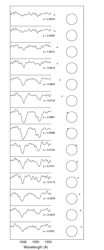
Figure 1: Series of IUE high resolution spectra of C iv UV mult. 1 and the corresponding positions of the B star behind the primary as seen from Earth. The spectra are smoothed with a Savitzky-Golay filter

Table 2: Orbital elements and stellar parameters of HR 6902 [gathered from Griffin et al. (1995); the distance is obtained from the Hipparcos Main Catalog]

Parameter	Value
Period (days)	385.0
Eccentricity	0.311
Inclination (deg)	87
Longitude of periastron (deg)	146
Semimajor axis (cm)	$\mathrm{\,2.94\times 10^{13}}$
Periastron passage (JD)	2 447 306.33
Conjunction (JD)	2 447 788.18
Spectral type (primary)	G9 IIb
Spectral type (secondary)	B8-9 V
$R_{\mathrm{G}}/\mathrm{{R_{\odot}}}$	33.0
$R_{\mathrm{B}}/\mathrm{{R_{\odot}}}$	3.0
$M_{\mathrm{G}}/\mathrm{{M_{\odot}}}$	3.86
$M_{\mathrm{B}}/\mathrm{{M_{\odot}}}$	2.95
$T_{\mathrm{eff,G}}$ (K)	4900
$T_{\mathrm{eff,B}}$ (K)	11 600
$M_{\mathrm{V,G}}$ (mag)	$-1.81$
$M_{\mathrm{V,B}}$(mag)	$-0.03$
$E_{\mathrm{B-V}}$(mag)	$-0.18$
Distance (pc)	$247\pm 40$

Great significance must be attached to the emission line spectrum visible during total eclipse of the B star. The 1988 total eclipse observation (SWP 34143, $\phi=0.998$) was part of the first HR 6902 program and has been reported by Reimers et al. (1990a). The deep $410^{\rm m}$ exposure SWP 39795 (Fig. 2) obtained on 1990 October 8 provides a significantly improved signal-to-noise ratio and will be subject of this paper. We note that the large difference in quality does not allow a comparative analysis in order to search for long-term variations. While in ”normal” $\zeta$ Aur systems hundreds of scattering lines (e.g., Fe ii and Si ii) are seen, only a few are observed in the spectrum of HR 6902. A comparison with stars of similar spectral type suggests that the emission line spectrum cannot be due to the G star alone (Reimers et al. 1990a ). Instead, the observed C iv and Si iv doublets are formed primarily by resonance scattering of B star photons in the circumstellar envelope.

Griffin et al. (1995) have redetermined the orbital and stellar parameters of HR 6902 by means of photometric observations during the eclipses of 1987 and 1989 (Table 2). The relative orbit and the eclipse geometry are shown in Fig. 3. It should be noted that the stellar parameters of giants belonging to $\zeta$ Aur systems can be much better determined than for single stars. A recent evolutionary analysis suggests that the bright giant primary of HR 6902 is already evolved into its blue loop phase (Schröder et al. (1997)).

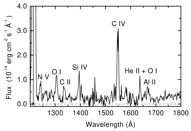
Figure 2: IUE low resolution spectrum SWP 39795 obtained at phase $\phi=0.9997$ showing the C iv and Si iv resonance doublets and a number of additional emission lines

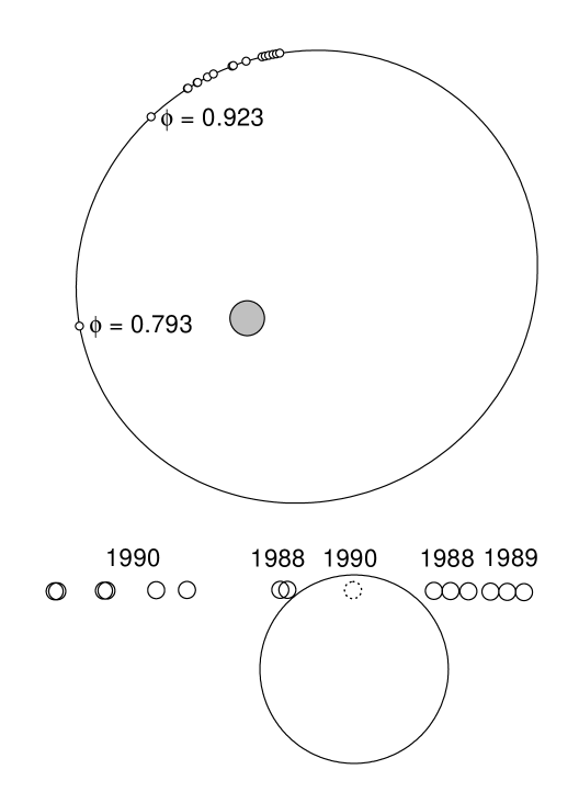
Figure 3: Relative orbit and binary geometry for all phases with detectable Si iv and C iv lines

3 Absorption line diagnostics

A comparison of the total eclipse emission line spectrum with the out-of-eclipse observations shows immediately that the continuum flux is orders of magnitude larger than the scattered line flux. Hence, the circumstellar absorption profiles can be interpreted as pure absorption lines formed in the extended envelope of HR 6902. In the subsequent sections we present details of the analysis and interpretation of the spectra of HR 6902.

3.1 Basic equations

The line formation in HR 6902 is dominated by velocity fields on different scales. To simplify the concept we introduce a line broadening velocity $v_{\rm b}$ containing both the thermal velocity $v_{\rm th}$ and a stochastic component $v_{\rm sto}$ associated with turbulence or other short-scale nonthermal motions. Assuming a Gaussian distribution of the stochastic velocity the spectroscopic line broadening parameter becomes $v_{\rm b}^{2}=v_{\rm th}^{2}+v_{\rm sto}^{2}$. The macroscopic velocity field is characterized by a spherically symmetric expansion described by an a priori unknown velocity law $v_{\rm wind}(r)$.

Throughout this paper we assume the line broadening velocity to be constant in the relevant parts of the envelope. It is convenient to define a dimensionless frequency variable $x=(\nu-\nu_{0})/\Delta\nu_{\rm d}$, where $\nu_{0}$ is the line-center frequency and $\Delta\nu_{\rm d}=\nu_{0}v_{\rm b}/{\rm c}$ the corresponding Doppler width. Macroscopic velocities are measured in the same units, i.e. $u(r)=v(r)/v_{\rm b}$. Regarding the B star as a point light-source of intensity $I_{\rm B}$ the emergent flux for a given impact parameter $p$ can be written

$$F_{x}(p)=I_{\rm B}\exp\left[-\tau_{x}(p)\right].$$ (1)

The optical depth along a ray from the observer to the B star is given by

$$\tau_{\rm x}(p)=k_{\rm 0}\int_{z_{min}}^{z_{max}}n(r)\Phi\left[x-\frac{z}{r}u(r)\right]\,\rm{d}z,$$ (2)

where $\Phi(x)$ denotes the dimensionless profile function. The geometry is defined by the distance from the primary $r$ and the integration path $z=\sqrt{r^{2}-p^{2}}$. The boundaries $z_{min}$ and $z_{max}$ depend on the position of the B star and the adopted outer radius of the envelope (chosen as large that the results are unaffected by its actual value), respectively. The line opacity per absorber reads

$$k_{\rm 0}=\frac{\pi\rm{e^{2}}}{\rm{m_{e}}c}\lambda_{0}fv^{-1}_{\rm sto},$$ (3)

where $f$ is the oscillator strength and $\lambda_{0}$ the rest wavelength of the transition under consideration.

In the static case (i.e. without considering the expansion explicitly) Eq. 2 degenerates to a simple relation between the optical depth and the column density $N$, viz

$$\tau_{\rm x}(p)=k_{\rm 0}N\Phi(x).$$ (4)

Our analysis is carried out using a non-linear least square fit technique based on the Levenberg-Marquard method (e.g., Press et al. (1992)) to derive the column density $N$ and the line broadening parameter $v_{\rm sto}$. The NEWSIPS error estimate provides statistical errors of the deduced parameters and allows to assess the goodness-of-fit. As an additional constraint the best-fit parameters are forced to be equal for all lines of the particular multiplet under consideration, i.e., we favor the strategy of resonance doublet modeling instead of analyzing individual absorption lines. Our fitting procedure allows to vary the continuum flux level in order to avoid the difficulties associated with a continuum definition by eye. Finally, the theoretical profile has to be convoluted with the IUE line-spread function. The instrumental profile is assumed to be well represented by a Gaussian with FWHM in accordance with the actual determination of the NEWSIPS resolution (Garhart et al. (1997)).

3.2 Quasi-static approach

As a starting point of our analysis we use a quasi-static approximation neglecting macroscopic velocity fields. The objective of this approach is to provide a provisional set of column densities and stochastic velocities. However, line broadening effects due to the wind outflow calls the static model into question. In Sect. 3.3 we will examine possible consequences for the derived parameters.

In the spectrum SWP 31325 (impact parameter $p=5.2\;{\rm R_{g}}$) we cannot identify any signature of C iv or Si iv absorption lines. Instead, we use the error information of the IUE flux to determine upper limits of the column densities. The results of the static analysis are summarized in Table 3. Fig. 4 shows the run of column densities as a function of the impact parameter. As already noticed by Reimers et al. (1990b), the egress observations indicate significant differences from epoch to epoch. The obtained stochastic velocities show a considerable scatter with a weighted mean of $68\pm 16\;{\rm km\,s}^{-1}$.

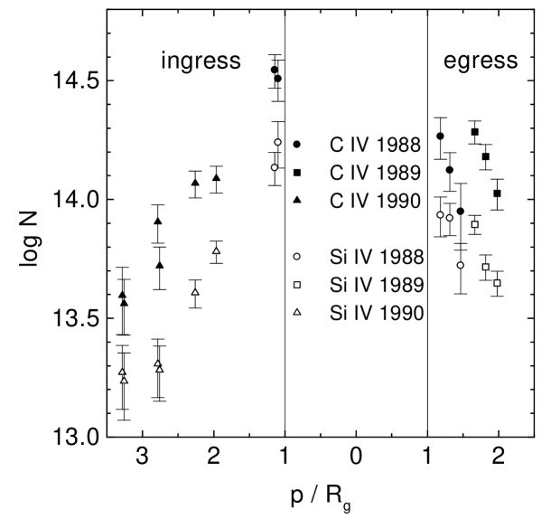
Figure 4: Column densities of ${C\textsc{iv}}$ and ${Si\textsc{iv}}$ obtained by the quasi-static approach

Table 3: Column densities, stochastic velocities, and temperatures derived from least square profile modeling. The parameters are obtained using two distinct wind models. At each phase the first line displays the results of the quasi-static approach. The second line shows the effect of the macroscopic velocity field ($\beta$ power-law with $v_{\infty}=100\;\mathrm{km\,s^{-1}}$). Additional information can be found in the text

Phase	$\log N[{Si\textsc{iv}}]$	$\log N[{C\textsc{iv}}]$	$v_{\mathrm{sto}}(\mathrm{km\,s^{-1}})$	$T(10^{3}\,\mathrm{K})$	$\log N[\mathrm{H}]$
$0.9227$	$\leq 12.95$	$\leq 13.30$	–	–	–
$0.9534$	$13.27$ ($+0.11,-0.15$)	$13.60$ ($+0.12,-0.16$)	$101.9$ ($\pm$ 23.1)	$76.4$ ($\pm$5.0)	$18.08$ ($+0.18,-0.11$)
	$13.25$ ($+0.10,-0.13$)	$13.59$ ($+0.10,-0.13$)	$62.7$ ($\pm$ 29.4)	$76.4$ ($\pm$5.3)	$18.06$ ($+0.15,-0.12$)
$0.9538$	$13.24$ ($+0.12,-0.16$)	$13.56$ ($+0.10,-0.13$)	$64.0$ ($\pm$ 23.0)	$76.4$ ($\pm$4.5)	$18.04$ ($+0.18,-0.12$)
	$13.23$ ($+0.11,-0.14$)	$13.59$ ($+0.10,-0.13$)	$65.5$ ($\pm$ 31.7)	$77.3$ ($\pm$5.6)	$18.04$ ($+0.17,-0.14$)
$0.9612$	$13.31$ ($+0.11,-0.14$)	$13.90$ ($+0.07,-0.09$)	$103.3$ ($\pm$ 16.2)	$82.2$ ($\pm$3.2)	$18.16$ ($+0.19,-0.12$)
	$13.32$ ($+0.10,-0.13$)	$13.91$ ($+0.06,-0.07$)	$74.0$ ($\pm$ 20.3)	$82.2$ ($\pm$3.7)	$18.17$ ($+0.16,-0.16$)
$0.9616$	$13.28$ ($+0.10,-0.13$)	$13.72$ ($+0.08,-0.10$)	$58.5$ ($\pm$ 12.5)	$78.9$ ($\pm$3.2)	$18.10$ ($+0.15,-0.11$)
	$13.30$ ($+0.10,-0.12$)	$13.77$ ($+0.08,-0.09$)	$48.8$ ($\pm$ 22.3)	$79.4$ ($\pm$4.1)	$18.13$ ($+0.16,-0.16$)
$0.9694$	$13.61$ ($+0.05,-0.06$)	$14.07$ ($+0.05,-0.06$)	$64.2$ ($\pm$ 5.9)	$79.4$ ($\pm$1.9)	$18.43$ ($+0.08,-0.06$)
	$13.59$ ($+0.05,-0.06$)	$14.02$ ($+0.05,-0.06$)	$42.1$ ($\pm$ 11.8)	$78.9$ ($\pm$2.4)	$18.40$ ($+0.08,-0.07$)
$0.9742$	$13.78$ ($+0.04,-0.05$)	$14.09$ ($+0.05,-0.06$)	$67.7$ ($\pm$ 6.9)	$75.9$ ($\pm$1.8)	$18.59$ ($+0.05,-0.04$)
	$13.74$ ($+0.04,-0.05$)	$14.03$ ($+0.05,-0.05$)	$32.3$ ($\pm$ 10.3)	$75.7$ ($\pm$2.3)	$18.56$ ($+0.05,-0.04$)
$0.9887$	$14.13$ ($+0.06,-0.08$)	$14.54$ ($+0.07,-0.09$)	$71.9$ ($\pm$ 4.9)	$78.3$ ($\pm$2.4)	$18.95$ ($+0.09,-0.07$)
	$14.11$ ($+0.07,-0.08$)	$14.55$ ($+0.07,-0.08$)	$46.1$ ($\pm$ 9.4)	$78.9$ ($\pm$3.0)	$18.93$ ($+0.10,-0.09$)
$0.9898$	$14.24$ ($+0.09,-0.11$)	$14.51$ ($+0.08,-0.10$)	$64.1$ ($\pm$ 4.9)	$75.0$ ($\pm$3.2)	$19.05$ ($+0.13,-0.10$)
	$14.18$ ($+0.08,-0.10$)	$14.54$ ($+0.09,-0.11$)	$39.3$ ($\pm$ 11.4)	$77.3$ ($\pm$4.3)	$18.99$ ($+0.13,-0.10$)
$0.0122$	$13.93$ ($+0.08,-0.09$)	$14.27$ ($+0.08,-0.10$)	$51.4$ ($\pm$ 5.0)	$76.6$ ($\pm$3.0)	$18.74$ ($+0.10,-0.07$)
	$13.92$ ($+0.07,-0.08$)	$14.19$ ($+0.07,-0.08$)	$26.2$ ($\pm$ 12.9)	$75.0$ ($\pm$3.6)	$18.73$ ($+0.08,-0.05$)
$0.0147$	$13.92$ ($+0.06,-0.07$)	$14.12$ ($+0.08,-0.09$)	$55.6$ ($\pm$ 5.3)	$73.3$ ($\pm$2.8)	$18.75$ ($+0.11,-0.09$)
	$13.87$ ($+0.06,-0.07$)	$14.07$ ($+0.07,-0.08$)	$29.5$ ($\pm$ 13.6)	$73.4$ ($\pm$3.4)	$18.69$ ($+0.07,-0.05$)
$0.0175$	$13.72$ ($+0.09,-0.12$)	$13.95$ ($+0.12,-0.16$)	$45.2$ ($\pm$ 12.4)	$74.1$ ($\pm$4.8)	$18.54$ ($+0.19,-0.13$)
	$13.67$ ($+0.09,-0.11$)	$13.81$ ($+0.15,-0.23$)	$34.7$ ($\pm$ 24.1)	$72.0$ ($\pm$6.2)	$18.50$ ($+0.17,-0.12$)
$0.0209$	$13.89$ ($+0.04,-0.04$)	$14.28$ ($+0.05,-0.05$)	$101.2$ ($\pm$ 6.7)	$78.0$ ($\pm$1.5)	$18.70$ ($+0.05,-0.05$)
	$13.89$ ($+0.04,-0.04$)	$14.27$ ($+0.04,-0.05$)	$71.8$ ($\pm$ 9.5)	$77.8$ ($\pm$1.8)	$18.70$ ($+0.05,-0.04$)
$0.0235$	$13.72$ ($+0.05,-0.06$)	$14.18$ ($+0.05,-0.06$)	$101.2$ ($\pm$ 15.0)	$79.4$ ($\pm$1.7)	$18.54$ ($+0.07,-0.06$)
	$13.71$ ($+0.04,-0.05$)	$14.17$ ($+0.05,-0.05$)	$74.7$ ($\pm$ 17.5)	$79.3$ ($\pm$2.0)	$18.53$ ($+0.07,-0.06$)
$0.0261$	$13.65$ ($+0.05,-0.06$)	$14.03$ ($+0.06,-0.07$)	$95.9$ ($\pm$ 9.0)	$77.6$ ($\pm$2.0)	$18.46$ ($+0.06,-0.05$)
	$13.64$ ($+0.05,-0.05$)	$14.03$ ($+0.06,-0.06$)	$59.4$ ($\pm$ 15.4)	$77.8$ ($\pm$2.6)	$18.45$ ($+0.07,-0.06$)

Assuming the simplifying conditions of a low density plasma the C iv and Si iv density ratio can be used to derive an ionization temperature $T_{\mathrm{ion}}$. We solve the ionization balance using the radiative-collisional equilibrium program CLOUDY (version 9003; Ferland (1997)). The metal abundances are supposed to be solar ($A_{\rm C}=3.6\times 10^{-4},A_{\rm Si}=3.6\times 10^{-5}$ [Anders & Grevesse (1989)]). As an approximation we identify the ionization temperature with the kinetic temperature $T_{\mathrm{e}}$ knowing that the ionization state may freeze in, so that we have $T_{\mathrm{e}}\neq T_{\mathrm{ion}}$ in the outer wind. It turns out that the electron temperature appears to be constant within the observed part of the envelope ($p=1.1-3.3\;{\rm R_{g}}$) with a weighted mean of $T_{\rm e}=78\,000\pm 2000\;{\rm K}$. However, the ion ratio may be affected by different CNO abundances due to the first dredge up which can deplete the carbon abundance significantly (e.g., Lambert (1981)). For example, a carbon abundance reduced by a factor of 4 would lead to a temperature of $\sim 90\,000\;{\rm K}$.

3.3 Density models

With known electron temperature we are able to transform the ion density into total hydrogen densities. In the next step we try to match the derived hydrogen column densities employing different types of density laws. Each density law implies a physical model defined by a specific set of parameters. Again we implement a least square fit procedure using the Levenberg-Marquard method.

3.3.1 Hydrostatic model

As a first attempt we use the hydrostatic equation for an isothermal plasma

$$n_{\rm H}(r)=n_{\rm 0}\exp\left(-\frac{r_{0}}{r}\,\frac{r-r_{0}}{H}\right),$$ (5)

where $r_{0}$ defines the bottom of the envelope with the corresponding hydrogen density $n_{\rm 0}$. $H$ denotes the density scale height. This approach is motivated by the fact that at least the subsonic region will be well represented by the hydrostatic density law. In order to fit the empirical column densities we adjust the density parameter $n_{\rm 0}$ and the scale height $H$. Identifying $r_{0}$ with the giant radius the least square procedure yields $n_{0}=5.0\pm 0.92\times 10^{6}\;\rm{cm^{-3}}$ and $H=3.4\pm 0.14\times 10^{11}\;{\rm cm}$.

The pressure may be composed of two parts, the thermal gas component and an effective turbulent pressure leading to the total dynamical pressure

$$P_{\rm tot}=\rho\left(\frac{{\rm k}T}{\mu m_{\rm H}}+\frac{v_{\rm turb}^{2}}{2}\right),$$ (6)

where $\mu$ is the mean molecular weight measured in units of the hydrogen mass. The velocity $v_{\rm turb}$ denotes an isotropic turbulent motion with a spatial scale smaller than the pressure scale height. Assuming the ionization equilibrium to be described by the physics of a low density plasma with $T_{\rm e}=78\,000\;{\rm K}$ we obtain $\mu=0.64$ [for solar composition according to Anders & Grevesse (1989)]. If we identify the stochastic velocity of $68\;{\rm km\,s^{-1}}$ with the turbulent velocity we obtain a scale height of $3.4\times 10^{11}$ cm, in agreement with the best-fit parameter of the hydrostatic model. However, at the impact parameter of $p=5.2\;{\rm R_{g}}$ the theoretical column density exceeds the observed upper limit by a factor of 3 (see Fig. 5). As expected the hydrostatic equation provides an adequate description of the inner shell ($p<3\;{\rm R_{g}}$), but overestimates the densities in the outer envelope considerably.

3.3.2 Kinematic model: $\beta$ power-law

A more realistic model of the large-scale density distribution requires an appropriate kinematic approach. We follow two different strategies to introduce a velocity law: an analytical $\beta$ power-law approach traditionally used in $\zeta$ Aurigae studies, and a hydrodynamic description of an isothermal, isoturbulent wind (where $P/\rho=\mathrm{const}$). For the sake of simplicity we adopt a steady, spherically symmetric outflow. We are aware of the fact that these assumptions may be a point of criticism, since the observations suggest a considerable variability. However, the amplitude of these variations are small and justify a kind of ”average” description.

The first kinematic model uses a velocity law proven to be adequate for different classes of stellar winds including the envelopes of evolved late-type stars. The analyses of several $\zeta$ Aur binaries suggest a velocity field of the form

$$v(r)=v_{\infty}\left(1-\frac{\rm R_{g}}{r}\right)^{\beta},$$ (7)

where $v_{\infty}$ is the terminal wind velocity and $\beta$ the acceleration parameter which defines the steepness of the spatial velocity gradient associated with the expansion. The wind velocity $v(r)$ increases monotonically outward and approaches the terminal velocity at large distances from the giant. The number density is assumed to vary in accordance to the equation of continuity. The hydrogen density becomes

$$n_{\rm H}(r)=n_{\beta}\left(\frac{\rm R_{g}}{r}\right)^{2}\left(\frac{r}{r-{\rm R_{g}}}\right)^{\beta},$$ (8)

where the density parameter $n_{\beta}$ is related to the mass-loss rate and terminal wind velocity:

$$n_{\beta}=\frac{\dot{M}}{4\pi v_{\infty}{\rm R^{2}_{g}}}\frac{X_{\rm H}}{m_{\rm H}}.$$ (9)

The hydrogen abundance by weight $X_{\rm H}$ is fixed at $0.70$ assuming solar chemical composition. The least square procedure yields a set of best-fit parameters $n_{\beta}=6.6\pm 0.7\times 10^{5}$ $\rm{cm^{-3}}$ and $\beta=0.60\pm 0.14$.

The small value of $\beta$ indicates a rapid acceleration to $\sim 0.5\,v_{\infty}$ within $1.5\;{\rm R_{g}}$. We note that the wind models of ”classical” $\zeta$ Aurigae systems ($\zeta$ Aur, 31 Cyg , 32 Cyg) indicate a gradual acceleration with $\beta$ in the range between 2.5 and 3.5 (e.g., Schröder (1985)). In the case of HR 6902 the terminal velocity eludes a spectroscopic determination, since we can only observe the tangential velocity component. The poor quality of the spectra does not allow the use of alternative velocity indicators like Mg ii absorption. As a consequence the mass-loss information is restricted to the ratio $\frac{\dot{M}}{v_{\infty}}$. The winds from hybrid stars show high terminal velocities (typically 50 to $150\;{\rm km\,s^{-1}}$) as measured by the circumstellar Mg ii absorption (e.g., Dupree & Reimers (1987)). Furthermore, the flow velocities of luminous cool stars are always less than the escape speed from the photosphere (for HR 6902 we find $v_{\rm esc}=211\;{\rm km\,s^{-1}}$). So we expect $v_{\infty}$ to lie in the range $50-200\;{\rm km\,s^{-1}}$. The corresponding mass-loss rate is $8\times 10^{-12}-3.4\times 10^{-11}\;{\rm M_{\odot}\,yr^{-1}}$ with a statistical error of $\sim 10\%$.

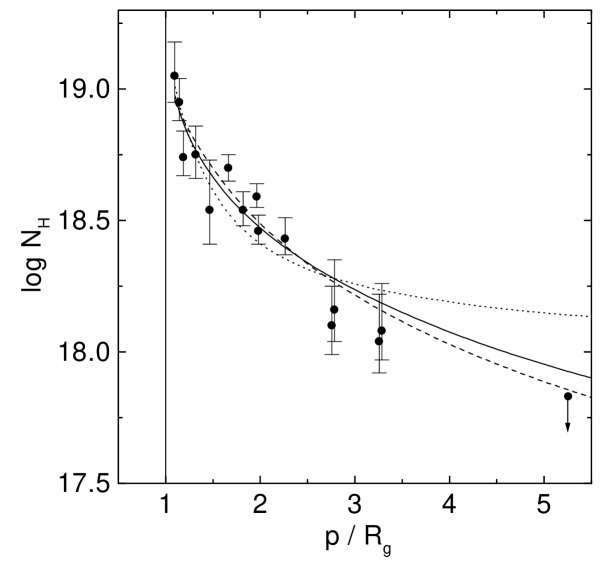
Figure 5: Comparison of best-fit density models with empirical hydrogen column densities (dotted: hydrostatic approach; solid: $\beta$ power-law; dashed: $P\propto\rho$ model)

3.3.3 Kinematic model: $P\propto\rho$ wind

Finally, we try to attack the mass motion using the equations of gas dynamics. Conservation of momentum gives the one-dimensional Euler equation

$$v\frac{{\rm d}v}{{\rm d}r}=-\frac{1}{\rho}\frac{{\rm d}P_{\rm eff}}{{\rm d}r}-\frac{{\rm G}{\rm M_{g}}}{r^{2}}+f(r),$$ (10)

where $f(r)$ denotes a potential extra force per unit-mass. In the present study we set $f=0$ and introduce an effective pressure term containing an unspecified nonthermal contribution assuming a proportionality of the form $P_{\rm eff}\propto\rho$. This simplification leads to a Parker-type wind. The Euler equation can be integrated immediately and yields a solution with a positive velocity gradient at all distances (e.g., Mihalas (1978)):

$$\frac{v}{v_{\rm c}}\exp\left[-\frac{1}{2}\left(\frac{v}{v_{\rm c}}\right)^{2}\right]=\left(\frac{r_{\rm c}}{r}\right)^{2}\exp\left(-\frac{2r_{\rm c}}{r}+\frac{3}{2}\right).$$ (11)

The transcendental equation can be solved numerically to give $v(r)/v_{\rm c}$. The critical radius is defined by the singularity of the Euler equation:

$$r_{\rm c}=\frac{{\rm G}{\rm M_{g}}}{2v^{2}_{\rm c}}.$$ (12)

The hydrogen density may be expressed by an equation of the form

$$n_{\rm H}(r)=n_{\rm c}\left(\frac{\rm R_{g}}{r}\right)^{2}\frac{v_{\rm c}}{v(r)},$$ (13)

where the density parameter $n_{\rm c}$ is related to the mass-loss rate by

$$n_{\rm c}=\frac{\dot{M}}{4\pi v_{\rm c}{\rm R}^{2}_{\rm g}}\frac{X_{\rm H}}{m_{\rm H}}.$$ (14)

This formalism suggests varying the density parameter and the critical velocity to model $n_{\mathrm{H}}(r)$. The critical velocity specifies the singularity of the momentum equation and thus determines the slope of the resulting density distribution. We note that there is no need to take explicitly care of specific pressure constituents. Our least square fit procedure yields $n_{\mathrm{c}}=1.5\pm 0.3\times 10^{6}\;{\rm cm^{-3}}$ and $v_{\mathrm{c}}=89.5\pm 13.7\;{\rm km\,s^{-1}}$. The density parameter leads to a mass-loss rate of $\dot{M}=3.4\pm 1.2\times 10^{-11}\;\rm M_{\odot}\,yr^{-1}$.

Using Eq. 12 the critical radius becomes $\sim 1.4\;{\rm R_{g}}$, indicating a high velocity close to the surface of the giant. Fig. 5 demonstrates that both wind models lead to similar density laws. Indeed, the approximate relationship between $v_{\rm c}$ and $\beta$ derived by Harper et al. [1995, Eq. (10)] yields an acceleration parameter of 0.54 quite similar to the result of our beta-law analysis. This finding may justify the $\beta$ power-law approach in other red giant winds, where we have an unknown hydrodynamic situation.

Assuming the effective pressure to be supplied by both gas and turbulence pressure the critical velocity is given by

$$v_{\rm c}=\sqrt{\frac{{\rm k}T}{\mu m_{\rm H}}+\frac{v^{2}_{\rm turb}}{2}}.$$ (15)

The best-fit model with $v_{\rm c}=89.5\;{\rm km\,s^{-1}}$ yields a turbulence of $v_{\rm turb}=119\;{\rm km\,s^{-1}}$ which exceeds the observed stochastic velocity by a factor of 1.8. This discrepancy may become even worse when we allow for macroscopic line broadening. Either the identification of turbulent and stochastic velocity is completely inappropriate, or the momentum Eq. 10 contains unknown external forces or pressure terms. Furthermore, the relation between the observed line broadening velocity and the turbulent velocity is not clear and depends on the driving mechanism(s), the geometry, and the statistics of the absorbing structures.

In the preceding analysis we have ignored line broadening due to the wind velocity. In order to examine the effect on the derived parameters we repeat the absorption line analysis with the complete optical depth quadrature according to Eq. 2. The wind outflow is assumed to be well described by the $\beta$ power-law. Again we consider terminal velocities ranging from 50 to $200\;{\rm km\,s^{-1}}$. It turns out that high velocity models with $v_{\infty}\gtrsim 150\;{\rm km\,s^{-1}}$ cannot reproduce the observed profile shapes adequately. The deduced stochastic component of the line broadening lies in the interval $20-100\;{\rm km\,s^{-1}}$ showing partly a large standard error. The range of stochastic velocities reflects both noisy IUE spectra and true irregularities of the local velocity field. As an example we present in Table 3 the results for $v_{\infty}=100\;{\rm km\,s^{-1}}$ which represents the most probable fit model. Though this model yields considerably reduced stochastic velocities with a weighted mean (i.e., averaged over all heights) of $47\pm 16\;{\rm{km\,s}^{-1}}$, the derived column densities are fairly close to the quasi-static model. This finding even holds for larger wind speeds and we conclude that the quasi-static analysis has produced column densities with a reasonable degree of confidence.

4 Emission line diagnostics

Reimers et al. (1990a) have shown that the C iv and Si iv emission lines are formed by resonance scattering of B star photons in the envelope of the primary. Profile modeling requires the solution of a two-dimensional radiative transfer problem. The difficulty arises due to the fact that the light source (i.e. the B star) is displaced from the center of wind symmetry. It is well-known that the scattering lines are formed in a large volume compared to the scale of the binary orbit (Baade et al. (1996)). Hence, the emission line diagnostics allows to study the large-scale properties of the circumstellar envelope.

For the 2-D radiative transfer calculations we employ the SEI (Sobolev with exact integration) method, i.e., the source function is approximated using the escape probability formalism followed by an exact formal solution using short characteristics. This procedure is simple in concept and can be applied to very extended geometrical grids. In normal $\zeta$ Aur systems the Sobolev approach leads to erroneous results, since the wind velocities are typically only a few times the stochastic velocities. However, a comparison with a more refined 2-D radiative transfer code (Baade (1989), 1990) demonstrates the reliability of the Sobolev solution in the case of HR 6902. The reason is the low mass-loss rate ($\dot{M}\approx 10^{-11}\;{\rm M_{\odot}\,yr^{-1}}$) compared to the ”classical” $\zeta$ Aur systems ($\dot{M}\approx 10^{-9}-10^{-8}\;{\rm M_{\odot}\,yr^{-1}}$). As a consequence the line opacities are small and multiple line photon scattering is of minor importance.

4.1 Sobolev approximation

In the framework of the first order escape probability theory the scattering integral is given by (e.g., Mihalas (1978))

$$\left<{J}\right>=[1-\beta({\bf r})]S({\bf r})+\beta_{\rm c}({\bf r})I_{\rm c},$$ (16)

where $I_{\rm c}$ denotes a constant core intensity representing the B star. The escape probabilities are given by

$$\beta({\bf r})=\frac{1}{4\pi}\int_{4\pi}\frac{1-\exp\left(-\tau_{\rm s}\right)}{\tau_{\rm s}}\,{\rm d}\Omega,$$ (17)

and

$$\beta_{\rm c}({\bf r})=\frac{1}{4\pi}\int_{\Omega_{\rm c}}\frac{1-\exp\left(-\tau_{\rm s}\right)}{\tau_{\rm s}}\,{\rm d}\Omega,$$ (18)

with the Sobolev optical thickness $\tau_{\rm s}=k_{0}n({\bf r})L({\bf r},{\bf n})$. The so-called Sobolev length in the direction ${\bf n}$ may be defined in tensor notation:

$$L({\bf r,n})=\left|\sum\limits_{ij}n_{i}n_{j}\frac{\partial u_{i}}{\partial r_{j}}\right|^{-1}.$$ (19)

The quantity $\beta({\bf r})$ denotes the probability that a photon emitted at the point $\bf{r}$ escapes from the outer boundary and $\beta_{\rm c}({\bf r})$ symbolizes the probability that a photon emitted by the core (i.e. the B star) penetrates to the point ${\bf r}$. In the case of pure resonance scattering the line source function is simply given by

$$S({\bf r})=\frac{\beta_{\rm c}({\bf r})I_{\rm c}}{\beta({\bf r})}.$$ (20)

Detailed information can be found in Hempe (1982) who applied the Sobolev formalism to the specific conditions of the binary configuration. With known source function on a two-dimensional grid, we can calculate the emergent radiation field. The intensities are supplied by the formal solution of the transfer equation and can be integrated along a set of parallel rays through the envelope. In a subsequent step the integration over all solid angles and normalization yields the residual flux $F_{\rm x}/F_{\rm c}$. For a detailed description we refer to Baade (1990) and Kirsch & Baade (1994).

4.2 Application to HR 6902

To calculate synthetic emission lines we extrapolate the wind models derived in Sect. 3 to the whole envelope assuming the temperature and thus the ionization state to remain fixed. Though this simplistic approach implies spurious energy sources to maintain the temperature it may be sufficient to explain qualitatively the observed flux.

In the first step we use the C iv and Si iv line ratio observed during total eclipse to derive the ionization temperature. Unfortunately, the clearly visible C ii line eludes the diagnostic procedure, since the photospheric background profile is not known precisely. Furthermore, the loci of line formation may be quite different. We calculate a grid of theoretical flux ratios in the temperature range between 60 000 and $90\,000\;{\rm K}$. The ionization problem is solved using the CLOUDY code as described in Sect. 3.2. To consider the influence of different wind velocities we have a closer look at four different models defined either by the $\beta$ power-law or the $P\propto\rho$ wind according to Sect. 3.3.

As shown in Fig. 6 the theoretical flux ratios depend only slightly on the specific wind model. The observed line ratio suggests an electron temperature of $T_{\rm e}=82\,500\pm 3000\;{\rm K}$ consistent with the mean temperature obtained on the basis of the absorption line analysis. We use the derived electron temperature to calculate integrated line fluxes of the C iv and Si iv emission lines. The observed values (Table 4) can be reconstructed using the parameters $n_{\beta}=2.9\times 10^{5}$ $\rm{cm^{-3}}$ for the $\beta$ power-law and $n_{\rm c}=8.3\times 10^{5}$ $\rm{cm^{-3}}$ for the $P\propto\rho$ wind model. In both cases the density parameter differs only by a factor of $\sim 2$ from the results of the absorption line analysis. The discrepancy may be a result of the inadmissible extrapolation of the isothermal density distribution. Indeed, we would expect a decreasing temperature at large distances from the giant causing a reduced absorber density.

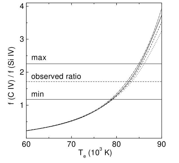
Figure 6: C iv$/$Si iv line flux ratio vs. electron temperature. The observed ratio is obtained from the total eclipse spectrum SWP 39795. The theoretical curves are presented for the $\beta$ power-law approach with different parameter sets [$\dot{M}({\rm M_{\odot}\,yr^{-1}}),v_{\infty}(\rm{km\,s^{-1}})$]: Solid [$8\times 10^{-12},50$], dashed [$1.7\times 10^{-11},100$], dotted [$3.4\times 10^{-11},200$]. The $P\propto\rho$ model is indicated by a dashed-dotted curve

Table 4: Observed emission line fluxes

Ion	$\lambda$	f
	(Å)	$(10^{-14}\,\mathrm{erg\,cm^{-2}\,s^{-1}})$
${Si\textsc{iv}}$	1395/1408	$14.2\pm 3$
${C\textsc{iv}}$	1548/1550	$24.7\pm 4$

The presence of a macroscopic velocity field will influence the profile shapes and cause wavelength shifts of the emission lines. However, the low resolution IUE spectra ($R\approx 6\;\mathrm{\AA}$) does not allow to examine these effects more closely. To demonstrate the expected situation we present in Fig. 7 a selection of theoretical flux profiles. It is obvious that the asymptotic flow velocity determines the character of the line profiles. In combination with a semi-empirical density model the line positions and profile shapes give reliable information about the global wind structure. This allows us to predict that high-resolution UV observations will unravel the kinematic nature of the circumstellar envelope of HR 6902.

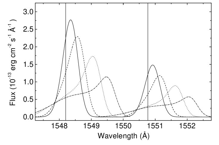
Figure 7: Theoretical line fluxes of the C iv resonance doublet during total eclipse ($\phi=1.000$). The line-center wavelengths are indicated by vertical lines. We present emergent profiles for the same wind models as shown in Fig. 6

5 Summary and discussion

In the present paper we have analyzed IUE observations of the $\zeta$ Aurigae type binary system HR 6902. The hot secondary serves as a convenient probe for the extended envelope of the bright giant. By means of a least square profile-fit procedure we have deduced C iv and Si iv column densities and stochastic velocities. The density distribution of the inner envelope ($\leq 3\;{\rm R_{g}}$) can be described by a quasi hydrostatic model. We have shown that pressure support by turbulence is sufficient to explain the empirical scale height. However, in order to match the empirical column densities adequately we had to introduce an appropriate outflow model. We have demonstrated that both the common $\beta$ power-law and a $P\propto\rho$ wind yield appropriate density distributions and explain the absence of C iv and Si iv absorption at larger distances from the giant. Fig. 8 demonstrates that the hydrostatic solution as well as the different outflow models lead to similar density laws. Despite this similarity the hydrodynamic implications are completely different. The required driving force per unit mass $f(r)$ should be compared to theoretical models.

We have derived mass-loss rates in the range $0.8-3.4\times 10^{-11}\;{\rm M}_{\odot}\,{\rm yr^{-1}}$. This result indicates that the mass-loss rate of HR 6902 scales roughly with the solar mass flux, i.e., $\dot{M}\approx\ {\rm\dot{M}_{\odot}(R_{g}/R_{\odot})^{2}}$. Finally, we have demonstrated that the emission line spectrum obtained during total eclipse confirms essentially the wind models derived from the absorption line analysis. This finding supports the picture of a steady and spherically symmetric flow without excessive deviations from the mean wind model.

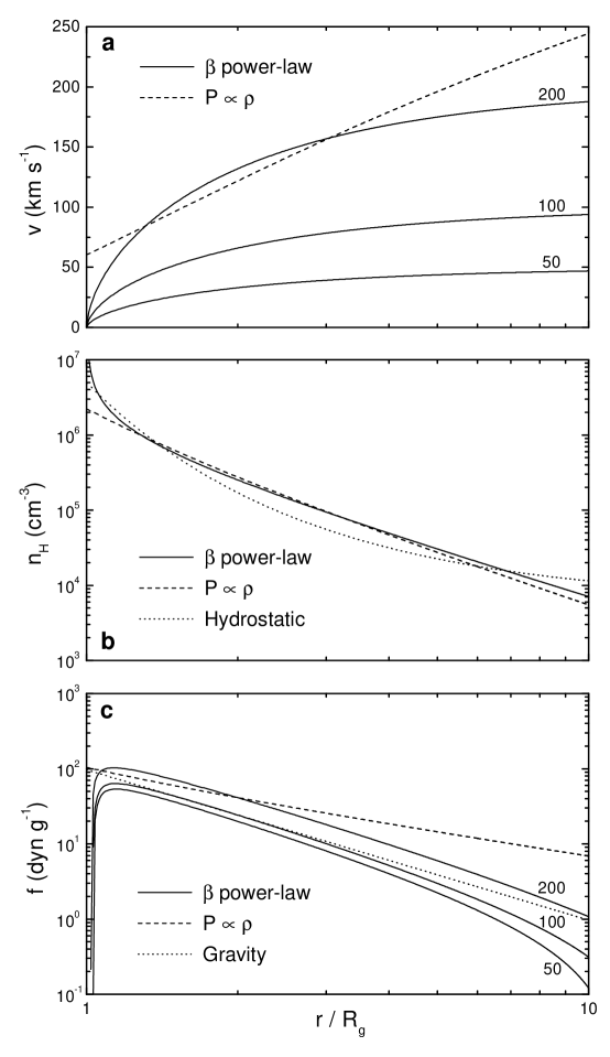
Figure 8: Velocity (a), density structure (b), and nonthermal momentum deposition (c) plotted as a function of radial distance. The $\beta$ power-law models are labelled with the corresponding terminal velocity

It is shown that HR 6902 possesses warm ($T_{\rm{e}}\approx 80\,000\;{\rm K}$) circumstellar material, observed in a range of impact parameters between 1.1 and $3.3\;{\rm R_{g}}$. Recently, the innermost region immediately above the photosphere ($p\leq 1.1\;{\rm R_{g}}$) has been examined by Schröder, Marshall, & Griffin (1996) using optical spectra. They derived a temperature of $T_{\rm{e}}\approx 5000\;{\rm K}$ and a turbulent velocity of $v_{\rm turb}=15\;{\rm km\,s^{-1}}$. However, in order to fit the Ca ii K-line wing they postulated a second absorption component with a considerably larger turbulent velocity of $\sim 45\;{\rm km\,s^{-1}}$ quite similar to the stochastic velocities derived in the present work. Combining these results we suspect a dramatic change of the physical conditions in the giant’s atmosphere at $p\approx 1.1\;{\rm R_{g}}$ associated with a steep rise of the temperature from about 5000 to $80\,000\;{\rm K}$.

The large nonthermal line broadening parameter and its relative constancy (apart from local fluctuations) may be a characteristic property of the wind of HR 6902. The simplistic identification of turbulence and the observed stochastic velocity cannot explain the large pressure required to explain the density distribution by a $P\propto\rho$ wind. However, the true relation between the observed line width and turbulent motions associated with wave-driven winds depends on the specific driving mechanism, geometrical details, and the randomness of the absorbing structures (e.g., Judge (1992)).

The wind models suggest a rapid wind acceleration within $\sim 0.5\;{\rm R_{g}}$ above the photosphere. This result is similar to the outflow characteristics of hybrid stars [$\alpha$ Aqr (G2 Ib), $\beta$ Aqr (G0 Ib), $\theta$ Her (K1 IIa), $\iota$ Aur (K3 II), $\gamma$ Aql (K 3II), and $\alpha$ TrA (K3 II); Brosius & Mullan (1986); Dupree et al. (1992); Harper et al. (1995)]. Furthermore, a recent analysis of ORFEUS II spectra of the hybrid stars $\alpha$ TrA and $\alpha$ Aqr (Dupree & Brickhouse (1998)) have revealed that the stellar winds are not confined to cool circumstellar material. They pointed out that ions like Si iii through O vi indicate expanding material up to a temperature of $3\times 10^{5}\;{\rm K}$ with wind velocities from 100 to $200\;\rm{km\,s^{-1}}$. We argue that the wind properties of hybrid stars are comparable to the extended atmosphere of HR 6902.

With its location in the HR diagram HR 6902 represents the physically important connection between solar-like stars with hot coronae and late type supergiants with cool outer atmospheres. The binary technique provides spatially resolved information about the physical structure of the extended envelope and wind that are unobtainable by other means. With IUE we have gained a first insight, but additional high resolution UV observations are indispensable to construct a detailed model. With this unique opportunity HR 6902 may play a crucial role in the elucidation of atmospheric heating processes and mechanisms to drive winds of cool stars.